Recognition of Affect in the wild using Deep Neural Networks
Dimitrios Kollias
?Mihalis A. Nicolaou
†Irene Kotsia
1,2Guoying Zhao
3Stefanos Zafeiriou
?,3?
Department of Computing, Imperial College London, UK
†Department of Computing, Goldsmiths, University of London, UK
3
Center for Machine Vision and Signal Analysis, University of Oulu, Finland
1School of Science and Technology, International Hellenic University, Greece
2
Department of Computer Science, Middlesex University, UK
?{s.zafeiriou, dimitrios.kollias15}@imperial.ac.uk, †
Abstract
In this paper we utilize the first large-scale ”in-the-wild” (Aff-Wild) database, which is annotated in terms of the valence-arousal dimensions, to train and test an end-to-end deep neural architecture for the estimation of continuous emotion dimensions based on visual cues. The proposed architecture is based on jointly training convolutional (CNN) and recurrent neural network (RNN) layers, thus exploiting both the invariant properties of convolutional features, while also modelling temporal dynamics that arise in human behaviour via the recurrent layers. Various pre-trained networks are used as starting structures which are subsequently appropriately fine-tuned to the Aff-Wild database. Obtained results show premise for the utilization of deep architectures for the visual analysis of human behaviour in terms of continuous emotion dimensions and analysis of different types of affect.
1. Introduction
Behavioral modeling and analysis constitute a crucial as-pect of Human Computer Interaction. Emotion recognition is a key issue, dealing with multimodal patterns, such as facial expressions, head pose, hand and body gestures, lin-guistic and paralinlin-guistic acoustic cues, as well as physi-ological data [19] [5] [18]. However, building machines which are able to recognize human emotions is a very chal-lenging problem. This is due to the fact that the emotion patterns are complex, time-varying, user and context de-pendent, especially when considering uncontrolled environ-ments, i.e., in-the-wild.
Currently, deep neural network architectures are the method of choise for learning-based computer vision, speech recognition and natural language processing tasks.
They have also achieved great performances in emotion recognition challenges and contests [23] [14] [13] [8]. Moreover, end-to-end architectures, i.e. networks that are trained, tested and subsequently utilized as systems applied on the raw input data, seem very promising for implement-ing platforms that can reach the market and be easily used by customers and users.
In this paper, we make a considerable effort to go beyond current practices in facial behaviour analysis, by training models on large scale data gathered in ”in-the-wild”, that is in entirely uncontrolled conditions. In more detail, we uti-lize the first, annotated in terms of continuous emotion di-mensions, large scale ”in-the-wild” database of facial affect, i.e. the Aff-Wild database [27]. Exploiting the abundance of data available in video-sharing websites, the database is enriched with spontaneous behaviours (such as subjects re-acting to an unexpected development in a movie or a series, a disturbing clip, etc.). The database contains more than 30 hours of video, and around 200 subjects.
Given the Aff-Wild data, we show that it is possible to build upon the recent breakthroughs in deep learning and propose, the first, to the best of our knowledge, end-to-end trainable system for valence and arousal estimation using ”in-the-wild” visual data1.
In the rest of the paper, we first describe briefly the Aff-Wild database (Section2), afterwards we present the pro-posed end-to-end deep CNN and CNN-RNN architectures (Section 3) and then the experimental results (Section4). Finally, conclusions and future work are presented in Sec-tion5.
1An end-to-end trainable Convolutional Neural Network (CNN) plus Recurrent Neural Network (RNN) for valence and arousal estimation from speech has been recently proposed in [25]. Furthermore, the recent method in [12] combines CNN with RNN (but independently trained) for valence and arousal in the AVEC data that have been captured in controlled condi-tions [22].
Figure 1: Annotated valence and arousal (Person A)
2. The Aff-Wild Database
Training and testing of the deep neural architectures has been performed using the Aff-Wild database [27]; this database shows spontaneous facial behaviors in arbitrary recording conditions, which should be analyzed so as to detect the valence and arousal emotion parameters. The database contains 298 videos of 200 people in total.
Figures 1, 2 show two characteristic sequences of facial images, taken from different videos of Aff-Wild. They include the respective video frame numbers and the valence and arousal annotations for each of them. A visual representation of the valence and arousal values is also depicted on the 2-D emotion space, showing the change in the reactions/behavior of the person among these time instances of the video. Time evolution is indicated, by using a larger size for the more recent frames and a smaller size for the older ones.
Figure3shows the histogram of valence and arousal an-notations. It can be seen that the amount of annotated pos-itive reactions, corresponding to pospos-itive valence values, is larger than that of negative ones. Similarly, the amount of annotated ’evident’ reactions, with positive arousal values, is larger than the less ’evident’, or hidden ones, with nega-tive arousal values. We examine in more detail this issue in the experimental section of the paper.
2.1. Database Pre-processing
The whole database contains more than 1,180,000 frames (around 900K for training and 300K for testing). From each frame, we detected faces using the method de-scribed in [15] and cropped the faces. Next, we applied the best performing method of [3] in order to track 68 facial
Figure 2: Annotated valence and arousal (Person B)
Figure 3: Histogram of Annotations
landmark. Since, many of the current pre-trained networks, such as VGG series of networks, operate on images with resolution of 224×224×3 we have always resized the facial images to this resolution.
In order to have a more balanced dataset for training, we performed data augmentation, mainly through dupli-cating [16] some data from the Aff-Wild database. To be more precise, we duplicated data that had negative valence and arousal values, as well as positive valence and nega-tive arousal values. As a consequence, the training set con-sisted of about 43% of positive valence and arousal values,
24% of negative valence and positive arousal values, 19% of positive valence and negative arousal values and 14% of negative valence and arousal values.
3. The End-to-End Deep Neural Architectures
We have developed end-to-end architectures, i.e., archi-tectures that trained all-together, accepting raw data colour images, learn to produce 2-D predictions of valence and arousal.In particular, we have evaluated the following architec-tures:
(1) An architecture based on the structure of the ResNet L50 network [9].
(2) An architecture based on the structure of the VGG Face network [20].
(3) An architecture based on the structure of the VGG-16 network [24].
We also considered two different approaches (a) an only frame based approach where only CNNs are trained and (b) CNN plus RNN end-to-end approaches that can exploit the dynamic information of the video data. In both settings, we present experimental results based on the following scenar-ios:
(1) The network is applied directly on cropped facial video frames of the generated database, trained to produce both valence and arousal (V, A) predictions.
(2) The network is trained on both the facial appearance video frames, as well as the facial landmarks corre-sponding to the same frame.
Regarding the CNN-RNN architecture, we utilize Long Short Term Memory (LSTM) [10] and Gated Recurrent Unit (GRU) [4] layers, stacked on top of the last fully con-nected layer. The RNN-LSTM/GRU consists of one or two hidden layers, along with the output layer that provides the final 2-D emotion predictions. We note that all deep learn-ing architectures have been implemented in the Tensorflow platform [1].
For training, we utilize the Adam optimizer, that pro-vides slightly better overall performance in comparison to other methods, such as the stochastic gradient descent. Fur-thermore, the utilized loss functions for evaluation and training include the Concordance Correlation Coefficient (CCC) and Mean Squared Error (MSE). We primarily fo-cus on optimizing the CCC, since it can provide better in-sight on whether the prediction follows the structure of the ground truth annotation. In more detail, the CCC is defined as ρc = 2sxy s2 x+s2y+ (¯x−y¯)2 (1)
where sx and sy are the variances of the predicted and ground truth values respectively,x¯andy¯are the correspond-ing mean values, whilesxandsy are the respective covari-ance values.
Regarding initialization, in our experiments we trained the proposed deep architectures by either (i) randomly ini-tializing the weight values, or (ii) using pre-trained weights from networks having been pre-trained on large databases, such as the ImageNet [6]. For the second approach we used transfer learning [17], especially of the convolutional and pooling part of the pre-trained networks. In more detail, we utilized the ResNet L50 and VGG-16 networks, which have been pre-trained for object detection tasks, along with VGG-Face, which has been pre-trained for face recognition tasks. In all experiments, the VGG-Face provided much better results, so, in the following we focus on the transfer learning methodology with weight initialization using the VGG-Face network; this has been pre-trained on the Face-Value dataset [2]. It should be noted that when utilizing pre-trained networks, we experimented based on two ap-proaches: either performing fine-tuning, i.e., training the entire architecture with a relatively small learning rate, or freezing the pre-trained part of the architecture and retrain-ing the rest (i.e., the fully connected layers of the CNN, as well as the hidden layers of the RNN). In general, the procedure of freezing a part of the network and fine-tuning [11] the rest can be deemed very useful, in particular when the given dataset is incremented with more videos. This in-creases the flexibility of the architecture, as fine-tuning can be performed by simply considering only the new videos. Training was performed on a single TITAN X (Pascal) GPU with a training time of around 5 days.
3.1. Implementing the CNN Architectures
In the following we provide specific information on the selected structure and parameters in the used end-to-end neural architectures, with reference to the results obtained for each case in our experimental study.
Extensive testing and evaluation has been performed by selecting different network parameter values, including (1) the number of neurons in the CNN fully connected layers, (2) the batch size used for network parameter updating, (3) the value of the learning rate and the strategy for reducing it during training (e.g. exponential decay in fixed number of epochs), (4) the weight decay parameter value, and finally (5) the dropout probability value.
With respect to parameter selection in the CNN archi-tectures, we used a batch size in the range 10−100 and an initial learning rate value in the range 0.0001−0.01 with ex-ponential decay. The best results have been obtained with batch size 80 and initial learning rate 0.001. The dropout probability value was 0.5, the decay steps of the exponen-tial decay of the learning rate were 400, while the learning
rate decay factor was 0.97. The number of neurons per layer per CNN type is described in the next subsections.
3.1.1 CNN architecture based on ResNet L50
Table 1 shows the configuration of the CNN architecture based on ResNet L50. This is composed of 9 blocks. For each convolutional layer the parameters are denoted as (channels, kernel, stride) and for the max pooling layer as (kernel, stride). The bottleneck modules are defined as in [9]. For the fully connected layers, Table1 shows the respective number of units. Using three Fully-Connected (FC) layers was found to provide best results.
Table 1: Architecture for CNN network based on ResNet L50
block 1 1×conv layer (64,7×7,2×2) batch norm layer
1×max pooling (3×3,2×2) block 2 3×bottleneck [(64,1×1), (64,3×3), (256,1×1)] block 3 4×bottleneck [(128,1×1), (128,3×3), (512,1×1)] block 4 6×bottleneck [(256,1×1), (256,3×3), (1024,1×1)] block 5 6×bottleneck [(512,1×1), (512,3×3), (2048,1×1)] block 6 1×average pooling
block 7 fully connected 1 1500 dropout layer
block 8 fully connected 2 256 dropout layer
block 9 fully connected 3 2
Table1refers to our second scenario where both the out-puts of the last pooling layer of the CNN, as well as the 68 landmark 2-D positions (68×2 values) were provided as inputs to the first of the three fully connected (FC) layers of the architecture. In the contrary, in scenario (1), the outputs of the last pooling layer of the CNN were the only inputs of the fully connected layer of our architecture. In this case, the architecture included only two fully connected layers, i.e., the 1st and 3rd fully connected ones.
In general, we used 1000 −1500 units in the first FC layer and 200−500 units in the second FC layer. The last layer consisted of 2 output units, providing the (V, A) pre-dictions. A linear activation function was used in this last FC layer, providing the final estimates. All units in the other
FC layers were equipped with the rectification (ReLU) non-linearity.
3.1.2 CNN architecture based on VGG-Face/VGG-16
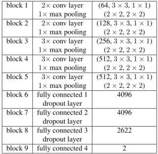
Table 2 shows the configuration of the CNN architecture based on VGG-Face or VGG-16. It is also composed of 9 blocks. For each convolutional layer the parameters are de-noted as (channels, kernel, stride) and for the max pooling layer as (kernel, stride). Table2shows the respective num-ber of units of each fully connected layer. Using four fully connected layers was found to provide best results. Table 2: Architecture for CNN network based on VGG-Face/VGG-16
block 1 2×conv layer (64,3×3,1×1)
1×max pooling (2×2,2×2) block 2 2×conv layer (128,3×3,1×1)
1×max pooling (2×2,2×2) block 3 3×conv layer (256,3×3,1×1)
1×max pooling (2×2,2×2) block 4 3×conv layer (512,3×3,1×1)
1×max pooling (2×2,2×2) block 5 3×conv layer (512,3×3,1×1)
1×max pooling (2×2,2×2) block 6 fully connected 1 4096
dropout layer
block 7 fully connected 2 4096 dropout layer
block 8 fully connected 3 2622 dropout layer
block 9 fully connected 4 2
Table2also refers to the second scenario. In this case, however, best results were obtained, when the 68 landmark 2-D positions (68×2values) were provided, together with the outputs of the first FC layer of the CNN, as inputs to the second of the four FC layers of the architecture. In sce-nario 1, the outputs of the first FC layer of the CNN were the only inputs to the second fully connected layer of our architecture. In this case, the architecture included only 3 FC layers, i.e., the 1st, 2nd and 4th FC layers. A linear acti-vation function was used in the last FC layer, providing the final estimates. All units in the rest FC layers were equipped with the rectification (ReLU) non-linearity.
3.2. Implementing the CNN-RNN architectures
When developing the CNN-RNN architecture, the RNN part was fed with the outputs of either the first, or the second fully connected layer of the respective CNN network. The structure of the RNN, which we examined, consisted of one or two hidden layers, with100-150units, following either
the LSTM neuron model allowing peephole connections, or the GRU neuron model. Using one fully connected layer in the CNN part and two hidden layers in the RNN part was found to provide the best results.
Table 3 shows the configuration of the CNN-RNN ar-chitecture. The CNN part of this architecture is based on the convolutional and pooling layers of the CNN architec-tures described above (in subsection3.1). It is followed by a fully connected layer. Note that in the case of the second scenario, both the outputs of the last pooling layer of the CNN, as well as the 68 landmark 2-D positions (68×2 val-ues) were provided as inputs to this fully connected layer. For the RNN and fully connected layers, Table3shows the respective number of units.
Table 3: Architecture for CNN-RNN network based on con-volution and pooling layers of previously described CNN architectures
block 1 CNN’s conv & pooling parts block 2 fully connected 1 4096
dropout layer
block 3 RNN layer 1 128 dropout layer
block 4 RNN layer 2 128 dropout layer
block 5 fully connected 2 2 Long evaluation has been performed by selecting differ-ent network parameter values. These parameters included: the batch size used for network parameter updating; the value of the learning rate and the strategy for reducing it during training (e.g. exponential decay in fixed number of epochs); the weight decay parameter value; the dropout probability value. Final selection of these parameters was similar to the CNN cases, apart from the batch size which was selected in the range100(≈3 seconds) -300(≈9 sec-onds). Best results have been obtained with batch size100.
4. Experimental Results
In the following, we provide the main outcomes of the experimental study, illustrating the above-described cases and scenarios. In all experiments training and validation was performed in the training set of the Aff-Wild database, while testing was performed in the test set of Aff-Wild. The first approach we tried was based on extracting SIFT fea-tures [26] from the facial region and then using an Support Vector Regression (SVR) [7] for valence and arousal esti-mation. For training and testing the SVRs, we utilized the scikit-learn library [21]. Obtained results were very poor. In particular, in all cases, the obtained CCC values were very low, while very low variance was present in the correspond-ing predictions (we do not present the performance of SVR
in order not to clutter the results).
4.1. Only-CNN architectures
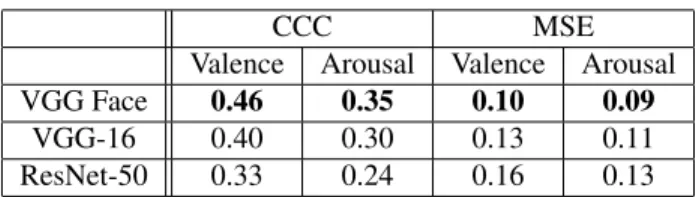
Table4summarizes the obtained CCC and MSE values on the test set of Aff-Wild using each of the three afore-mentioned CNN structures as pre-trained networks. The best results have been obtained using the VGG Face pre-trained CNN for initialization as shown in Table4. There-fore, we focus on utilizing this configuration for the results presented in the rest of this section. Moreover, Table 5 shows that there is a significant improvement in the per-formance, when we also use the 68 2-D landmark positions as input data (case with landmarks). It should be also noted that we have examined the following scenarios (a) having one network for joined estimation of valence and arousal and (b) estimation of the values of valence and arousal us-ing two different networks (one for valence and one for arousal). Slightly better results were obtained on the lat-ter case; so, this architecture is being used in the following results.
Furthermore, we have trained the networks with two dif-ferent annotations. The first is the annotation provided by the Aff-Wild database, which is the average over some an-notators (please see the Aff-Wild[27]). The second is the annotation produced by only one annotator (the one with the highest correlation to the landmarks). Annotations coming from a single annotator are generally less smooth than av-erage over annotators. Hence, they are more difficult to be learned. The results are summarized in Table6. As it was expected it is better to train over the annotation provided by Aff-Wild[27].
Table 4: CCC and MSE evaluation of valence & arousal predictions provided by the CNN architecture when using 3 different pre-trained networks for initialization
CCC MSE
Valence Arousal Valence Arousal VGG Face 0.46 0.35 0.10 0.09
VGG-16 0.40 0.30 0.13 0.11 ResNet-50 0.33 0.24 0.16 0.13
Table 5: CCC and MSE evaluation of valence & arousal predictions provided by the best CNN network (based on VGG Face), with/without landmarks
With Landmarks Without Landmarks Valence Arousal Valence Arousal CCC 0.46 0.35 0.38 0.31 MSE 0.10 0.09 0.14 0.11
Table 6: CCC and MSE evaluation of valence & arousal predictions provided by the best CNN network (based on VGG Face), using either one annotators values or the mean of annotators values
1 Annotator Mean of Annotators Valence Arousal Valence Arousal CCC 0.35 0.25 0.46 0.35
MSE 0.18 0.14 0.10 0.09
Table 7: Comparison of best CCC and MSE values of va-lence & arousal provided by best CNN and CNN-RNN ar-chitectures
CCC MSE
Valence Arousal Valence Arousal CNN 0.46 0.35 0.10 0.09 CNN-RNN 0.57 0.43 0.08 0.06
Table 8: Effect of Changing Number of Hidden Units & Hidden Layers for CCC valence & arousal values in the CNN-RNN architecture
1 Hidden Layer 2 Hidden Layers Hidden Units Valence Arousal Valence Arousal
100 0.40 0.33 0.47 0.40 128 0.49 0.40 0.57 0.43
150 0.44 0.37 0.50 0.41
4.2. CNN plus RNN architectures
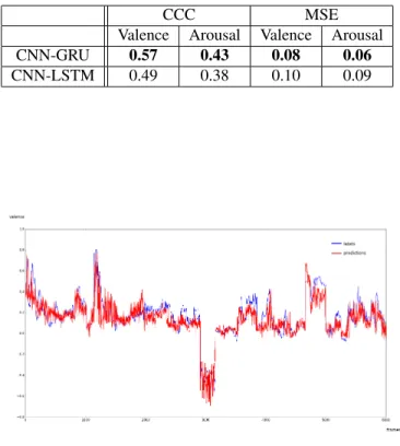
Let us now turn to the application of CNN plus RNN end-to-end neural architecture on Aff-Wild. We first per-form a comparison between two different units that can be used in an RNN network, i.e. an LSTM vs GRU. Table 9summarises the CCC and MSE values when using LSTM and GRU. It can be seen that best results have been obtained when the GRU model was used. All results reported in the following are, therefore, based on the GRU model. Table 7shows the improvement in the CCC and MSE values ob-tained when using the best CNN-RNN end-to-end neural ar-chitecture compared to the best only-CNN one. In particu-lar, we compare networks that take as input facial landmarks and are based on the pre-trained VGG Face network. It can be seen that this improvement is about 24% in valence esti-mation and about 23% in arousal estiesti-mation, which clearly indicates the ability of the CNN-RNN architecture to better capture the dynamic phenomenon.
We have tested various numbers of hidden layers and hidden units per layer when training and testing the CNN-RNN network. Some characteristic selections and the cor-responding CNN-RNN performances are shown in Table8. In Figures4and5, we qualitatively illustrate some of the
Table 9: CCC and MSE evaluation of valence & arousal predictions provided by the best GRU and CNN-LSTM architectures that had same network configurations (2 hidden layers with 128 units each)
CCC MSE
Valence Arousal Valence Arousal CNN-GRU 0.57 0.43 0.08 0.06
CNN-LSTM 0.49 0.38 0.10 0.09
Figure 4: Predictions vs Ground Truth for valence for a part of a video
Figure 5: Predictions vs Ground Truth for arousal for a part of a video
obtained results, comparing a segment of the obtained va-lence/arousal predictions compared to the ground truth val-ues, in over 6000 consecutive frames of test data.
5. Conclusions and future work
In this paper, we present the design, implementation and testing of deep learning architectures for the problem of analysing human behaviour utilizing continuous dimen-sional emotions. In more detail, we present, to the best of our knowledge, the first such architecture that is trained on hundred thousands of data, gathered ”in-the-wild” (i.e., in entirely uncontrolled conditions) and annotated in terms of continuous emotion dimensions. It should be empha-sized that a major challenge in facial expression and emo-tion recogniemo-tion lies in the large variability of spontaneous expressions and emotions, arising in uncontrolled environ-ments. This prevents pre-trained models and classifiers to be successfully utilized in new settings and unseen datasets. In the current paper, our focus has been on experiments in-vestigating the ability of the proposed deep CNN-RNN ar-chitectures to provide accurate predictions of the 2D emo-tion labels in a variety of scenarios, as well as with cross-database experiments. Presented results are very encourag-ing, and illustrate the ability of the presented architectures to predict the values of continuous emotion dimensions on data gathered ”in-the-wild”. Planned future work lies in extending the analysis to simultaneously interpret the be-haviour of multiple subjects appearing in videos, as well as to further extend the derived representations obtained by the CNN-RNN architectures for subject and setting specific adaptation.
6. Acknowledgments
The work of Stefanos Zafeiriou has been partially funded by the FiDiPro program of Tekes (project num-ber: 1849/31/2015). The work of Dimitris Kollias was funded by a Teaching Fellowship of Imperial College Lon-don. We would like also to acknowledge the contribution of the Youtube users that gave us the permission to use their videos (especially Zalzar and Eddie from The1stTake).
References
[1] M. Abadi, A. Agarwal, P. Barham, E. Brevdo, Z. Chen, C. Citro, G. S. Corrado, A. Davis, J. Dean, M. Devin, S. Ghe-mawat, I. Goodfellow, A. Harp, G. Irving, M. Isard, Y. Jia, R. Jozefowicz, L. Kaiser, M. Kudlur, J. Levenberg, D. Man´e, R. Monga, S. Moore, D. Murray, C. Olah, M. Schuster, J. Shlens, B. Steiner, I. Sutskever, K. Talwar, P. Tucker, V. Vanhoucke, V. Vasudevan, F. Vi´egas, O. Vinyals, P. War-den, M. Wattenberg, M. Wicke, Y. Yu, and X. Zheng. Tensor-Flow: Large-scale machine learning on heterogeneous sys-tems, 2015. Software available from tensorflow.org. [2] S. Albanie and A. Vedaldi. Learning grimaces by watching
tv.arXiv preprint arXiv:1610.02255, 2016.
[3] G. G. Chrysos, E. Antonakos, P. Snape, A. Asthana, and S. Zafeiriou. A comprehensive performance evaluation
of deformable face tracking” in-the-wild”. arXiv preprint arXiv:1603.06015, 2016.
[4] J. Chung, C. Gulcehre, K. Cho, and Y. Bengio. Empirical evaluation of gated recurrent neural networks on sequence modeling.arXiv preprint arXiv:1412.3555, 2014.
[5] C. Corneanu, M. Oliu, J. Cohn, and S. Escalera. Survey on rgb, 3d, thermal, and multimodal approaches for facial ex-pression recognition: History, trends, and affect-related ap-plications. IEEE transactions on pattern analysis and ma-chine intelligence, 2016.
[6] J. Deng, W. Dong, R. Socher, L.-J. Li, K. Li, and L. Fei-Fei. Imagenet: A large-scale hierarchical image database. InComputer Vision and Pattern Recognition, 2009. CVPR 2009. IEEE Conference on, pages 248–255. IEEE, 2009. [7] H. Drucker, C. J. Burges, L. Kaufman, A. Smola, V.
Vap-nik, et al. Support vector regression machines. Advances in neural information processing systems, 9:155–161, 1997. [8] I. Goodfellow, Y. Bengio, and A. Courville.Deep Learning.
MIT Press, 2016.http://www.deeplearningbook. org.
[9] K. He, X. Zhang, S. Ren, and J. Sun. Deep residual learn-ing for image recognition. InProceedings of the IEEE Con-ference on Computer Vision and Pattern Recognition, pages 770–778, 2016.
[10] S. Hochreiter and J. Schmidhuber. Long short-term memory. Neural computation, 9(8):1735–1780, 1997.
[11] H. Jung, S. Lee, J. Yim, S. Park, and J. Kim. Joint fine-tuning in deep neural networks for facial expression recognition. In Proceedings of the IEEE International Conference on Com-puter Vision, pages 2983–2991, 2015.
[12] P. Khorrami, T. Le Paine, K. Brady, C. Dagli, and T. S. Huang. How deep neural networks can improve emotion recognition on video data. InImage Processing (ICIP), 2016 IEEE International Conference on, pages 619–623. IEEE, 2016.
[13] A. Krizhevsky, I. Sutskever, and G. E. Hinton. Imagenet classification with deep convolutional neural networks. In Advances in neural information processing systems, pages 1097–1105, 2012.
[14] Y. LeCun, Y. Bengio, and G. Hinton. Deep learning.Nature, 521(7553):436–444, 2015.
[15] M. Mathias, R. Benenson, M. Pedersoli, and L. Van Gool. Face detection without bells and whistles. InEuropean Con-ference on Computer Vision, pages 720–735. Springer, 2014. [16] A. More. Survey of resampling techniques for improving classification performance in unbalanced datasets. arXiv preprint arXiv:1608.06048, 2016.
[17] H.-W. Ng, V. D. Nguyen, V. Vonikakis, and S. Winkler. Deep learning for emotion recognition on small datasets us-ing transfer learnus-ing. InProceedings of the 2015 ACM on International Conference on Multimodal Interaction, pages 443–449. ACM, 2015.
[18] M. A. Nicolaou, H. Gunes, and M. Pantic. Continuous pre-diction of spontaneous affect from multiple cues and modal-ities in valence-arousal space. Affective Computing, IEEE Transactions on, 2(2):92–105, 2011.
[19] M. Pantic and L. J. Rothkrantz. Automatic analysis of fa-cial expressions: The state of the art. Pattern Analysis and Machine Intelligence, IEEE Transactions on, 22(12):1424– 1445, 2000.
[20] O. M. Parkhi, A. Vedaldi, and A. Zisserman. Deep face recognition. InBMVC, volume 1, page 6, 2015.
[21] F. Pedregosa, G. Varoquaux, A. Gramfort, V. Michel, B. Thirion, O. Grisel, M. Blondel, P. Prettenhofer, R. Weiss, V. Dubourg, J. Vanderplas, A. Passos, D. Cournapeau, M. Brucher, M. Perrot, and E. Duchesnay. Scikit-learn: Ma-chine learning in Python. Journal of Machine Learning Re-search, 12:2825–2830, 2011.
[22] F. Ringeval, B. Schuller, M. Valstar, R. Cowie, and M. Pan-tic. Avec 2015: The 5th international audio/visual emotion challenge and workshop. InProceedings of the 23rd ACM international conference on Multimedia, pages 1335–1336. ACM, 2015.
[23] J. Schmidhuber. Deep learning in neural networks: An overview.Neural Networks, 61:85–117, 2015.
[24] K. Simonyan and A. Zisserman. Very deep convolutional networks for large-scale image recognition. arXiv preprint arXiv:1409.1556, 2014.
[25] G. Trigeorgis, F. Ringeval, R. Brueckner, E. Marchi, M. A. Nicolaou, B. Schuller, and S. Zafeiriou. Adieu features? end-to-end speech emotion recognition using a deep convo-lutional recurrent network. InAcoustics, Speech and Signal Processing (ICASSP), 2016 IEEE International Conference on, pages 5200–5204. IEEE, 2016.
[26] A. Vedaldi and B. Fulkerson. Vlfeat: An open and portable library of computer vision algorithms. InProceedings of the 18th ACM international conference on Multimedia, pages 1469–1472. ACM, 2010.
[27] S. Zafeiriou, D. Kollias, M. Nicolaou, A. Papaioannou, G. Zhao, and I. Kotsia. Aff-wild: Valence and arousal ‘in-the-wild’ challenge. InProceedings of the IEEE Confer-ence on Computer Vision and Pattern Recognition Workshop, 2017.