Silhouette Mapping

(1)

Silhouette Mapping

The Harvard community has made this

article openly available.

Please share

how

this access benefits you. Your story matters

Citation Gu, Xiangfeng, Steven J. Gortler, Hugues Hoppe, Leonard McMillan, Benedict J. Brown, and Abraham D. Stone. Silhouette Mapping. Harvard Computer Science Group Technical Report TR-1-99. Citable link http://nrs.harvard.edu/urn-3:HUL.InstRepos:23017274 Terms of Use This article was downloaded from Harvard University’s DASH

repository, and is made available under the terms and conditions applicable to Other Posted Material, as set forth at http://

nrs.harvard.edu/urn-3:HUL.InstRepos:dash.current.terms-of-use#LAA

(2)

Silhouette Mapping

Xianfeng Gu

Steven J. Gortler

Hugues Hoppe

Computer Science , Harvard Univ.

Microsoft Research

Leonard McMillan

Benedict J. Brown

Abraham D. Stone

MIT LCS Computer Graphics

CS, Harvard

Dept of Philosophy, Harvard

March 15, 1999

Harvard University, Computer Science Technical Report: TR-1-99

Abstract

Recent image-based rendering techniques have shown success in approximating detailed models using sampled images over coarser meshes. One limitation of these techniques is that the coarseness of the geometric mesh is apparent in the rough polygonal silhouette of the rendering. In this paper, we present a scheme for accurately capturing the external silhouette of a model in order to clip the approximate geometry.

Given a detailed model, silhouettes sampled from a discrete set of viewpoints about the object are collected into a silhouette map. The silhouette from an arbitrary viewpoint is then computed as the interpolation from three nearby viewpoints in the silhouette map. Pairwise silhouette interpolation is based on a visual hull approximation in the epipolar plane. The sil-houette map itself is adaptively simplified by removing views whose silsil-houettes are accurately predicted by interpolation of their neighbors. The model geometry is approximated by a pro-gressive hull construction, and is rendered using projected texture maps. The 3D rendering is clipped to the interpolated silhouette using stencil planes.

1 Introduction

In interactive 3D rendering there is a constant tension between model complexity and rendering speeds. Scenes with high geometric complexity are necessary for visual realism, but require high computational costs to achieve. This tension will not go away soon. To this end there has been considerable research into how to best use a given amount of rendering resources, and a number of successful approaches have been developed.

(3)

One such approach is level-of-detail rendering [18]. In this approach, more polygons are used for nearby objects than for distant objects, using more rendering resources where they produce the most visual impact. More complicated view based level of detail methods also use more poly-gons in the silhouette regions of models, since this typically produces the highest quality visual appearance [42, 20, 27].

Another such approach is texture mapping and its descendant image based rendering algo-rithms. In these methods, resources are used to create photometric appearances of high complexity using objects with low geometric complexity and fidelity.

Some of the most impressive results are obtained from systems that combine concepts from both of these approaches[6, 9, 24, 31, 41]. Cohen et al. [9] combine model simplification with texture and normal maps to produce objects with high visual complexity with modest rendering budgets. This combination of approaches works extremely well at representing the appearances of the interiors of objects. The one limitation of these approaches is that they do a poor job of displaying high quality silhouettes of objects, since they use a low polygon count. This is unfortunate since the appearance of the silhouette of an object is one of the strongest visual cues as to the shape of an object [23].

To address this problem we have developed a rendering system that ensures that objects are displayed with high resolution silhouettes, even when low resolution geometry is used to speed up rendering. Like Cohen et al., we use simplified geometry to describe the objects’ shapes, and we use textures to create high visual complexity in the objects’ interiors. In our system, we introduce a silhouette clipping algorithm to ensure that the low resolution geometry is only drawn in the screen region defined by a high resolution silhouette. Silhouette clipping is an alternative to the view based level of detail methods such as [20], that must dynamically create a model simplified for the current view. These methods are quite complicated, and for model consistency must generate high polygon counts in regions that are near but not on the silhouette.

The first challenge one must face in order to do silhouette clipping is a way of quickly con-structing a high resolution silhouette for a given view. One could extract the silhouette dynamically by appealing to the high resolution geometry for each frame as done in [30, 16]. But these meth-ods compute all silhouette curves that separate front-facing polygons from back-facing polygons. Some of these curves lie in the interior of the model, and can not be used for silhouette clipping. We must be able to quickly compute only the boundary silhouettes (defined below).

Our system accomplishes the construction of a high resolution silhouette by using a precom-puted silhouette map. A silhouette map is a data structure completely independent of the original geometry that stores an explicit representation of the silhouette contour as seen from a discrete set of views. To obtain a silhouette for an arbitrary current view, three “nearby” silhouettes are extracted from this silhouette map. Silhouette interpolation is performed to create a silhouette for the current view. Thus, during the rendering of the current view, the data accessed and processed is on the order of the complexity of a silhouette contour, which is typically much less than the size of the high resolution model.1

1

As a rule of thumb, if the high resolution model hasnpolygons, and is tessellated evenly, the silhouette contour

is usually made up ofO( p

(4)

In some ways, the silhouette interpolation problem referred to above resembles the contour interpolation problem found in animation and morphing applications [38], which can be solved effectively with a number of ad hoc solutions. But silhouette interpolation is different from con-tour morphing in a few key ways. Silhouette concon-tours routinely undergo complicated topological changes as the viewpoint changes [23], and thus a silhouette interpolation method must be able to handle such cases routinely. Moreover, when there is a sharp feature point on the object, that point may remain on the silhouette of the nearby views. During silhouette interpolation, these points should be considered to be “in correspondence”. Typical contour morphing algorithms would not guarantee this. We have therefore developed a novel silhouette interpolation based on the epipolar geometry of two views. Our method can handle topological changes, and it ensures that actual feature points on silhouettes are treated as being in correspondence. Moreover, unlike the many existing contour morphing methods, our silhouette interpolation algorithm has a clear geometric interpretation. It also guarantees that the resulting interpolated silhouette contour is conservative: it is guaranteed to lie outside the actual silhouette that would be observed from the current view.

For typical objects, the silhouettes can change rapidly in some region of view space, and slowly in others. This happens for both geometric and topological reasons.

In areas of low surface curvature, the silhouette (when seen in 3D) slips quickly across the surface as the view changes, while in areas of high curvature, the silhouette moves slowly across the surface. In the limit, at sharp edges, the silhouette doesn’t move at all as the view position changes, until some change in global geometric configuration occurs.

When one considers both internal and external silhouettes portions (see terminology below), the topological changes that can occur for a silhouette are well understood [23]. As the view changes, the silhouette topology remains unchanged until a singular view is reached. At such a view a catastrophe occurs, and the topology of the silhouette changes according to well defined rules. When one only considers external silhouettes, as we do, the topological changes that occur cannot be analyzed as easily. Nevertheless, it should be clear that in certain regions, the silhouette undergoes discontinuous changes and interpolation becomes more difficult.

To address both of these problems, we have developed a silhouette map simplification algorithm that adaptively samples the view space. As a result, we keep more silhouette information in regions of view space where the silhouettes change most rapidly.

In order to perform silhouette clipping on the approximate geometry, one must have an ap-proximation that encloses a volume that is larger than the original geometry. To this end we have developed a progressive hull representation. This creates a nested family of approximating meshes with the property that each coarser mesh encloses the finer meshes. This representation is a variant of the progressive mesh representation [19] that uses linear programming to ensure the desired hull property.

Our silhouette map could also be used in cases where explicit high resolution geometry is not available, but high resolution silhouette information is. One such promising example is image based rendering. Extracting high quality depth information from images is a difficult problem; automatic (multi)stereo algorithms are notoriously unreliable, and even the heartiest of graduate students quickly tires from manually specifying the necessary correspondence points. In contrast,

(5)

the silhouette of an object can be extract from an image easily and with high accuracy.

Contributions

Our work has a number of distinct contributions

We introduce the idea of silhouette clipping, to efficiently render low resolution geometric

objects with high resolution silhouettes .

We introduce the idea of a silhouette map, which is an auxiliary data structure that stores the

silhouette appearance from a number of sampled viewpoints.

We describe an algorithm for silhouette interpolation. This algorithm, which is based on

epipolar geometry can handle topological changes, keeps sharp feature points in correspon-dence, and guarantees a silhouette which is outside the actual silhouette .

We describe a greedy simplification algorithm that samples silhouette information most

densely in regions of view space where the most changes occur.

We describe a progressive hull data structure for representing a nested sequence of enclosing

approximate geometries. This representation may have other uses such as collision detection.

Limitations

Our work has several limitations and thus directions where future work is required.

Silhouette clipping can only be applied to external silhouettes . Internal silhouettes are

gen-erally not closed contours, and therefore cannot be used to create a clipping region. This results in visible artifacts where an object is self occluding. To solve this, some method for decomposing the original object into subobjects would be necessary.

Our interpolation method is conservative. Given the silhouettes recorded at three viewpoints

in space, our algorithm will produce a conservative silhouettes for any viewpoint on the triangle connecting the three vertices. The actual silhouette is guaranteed to lie within the interpolated silhouette , but is generally not on it. Our interpolation algorithm is based on the concept of visual hull, which is generally too conservative. In order to produce tighter silhouettes ideally would require higher order differential information about the surface at each point on the silhouettes .

Our algorithm is local, in that it only uses the nearest three views to create the interpolation.

While for some classes of contours it can be shown that this is optimal, in general there are cases where other farther views can improve the computation of the silhouettes of the visual hull. Further analysis is required.

(6)

The algorithm described in section 5.1 is an interpolation algorithm and not an extrapolation

algorithm. In order to compute correctly silhouettes that are not on a triangle (because the viewpoint has moved closer or farther from the object) would requires explicit depth information at each point on the silhouettes , or a tetrahedralization of space. In practice we use a simple planar homography (section 5) which we have found to work adequately well in practice.

Subdividing the intervals of a span into cliques requires correspondence between the

inter-vals in the two views. Our heuristic for this can be incorrect if multiple topological changes have occurred between the two views. In practice, this is taken care of by our silhouette map simplification algorithm. In regions where correspondence is difficult, denser samples are used. Again more analysis would be useful here.

Preliminaries

Silhouettes

In order to help our discussion, we will introduce here a small amount of terminology. For a pin hole imaging model and a smooth surface, a silhouette is created when a ray with direction vector

~r

passing through the pin hole touches the surface at a pointPwhere the normal of the surface is

orthogonal to the ray direction

~r

~n

P

=0

The set of 3D pointsPfor which this is true is called the contour generator. The contour generator

is generically made up of a set of smooth closed 3D contours on the surface [7]. The projection of the contour generator onto the image plane is called the apparent contour. The apparent contour is a 2D curve that can self intersect, and at some points (called cusps) it can be non-smooth. If we view the image of an opaque object, many parts of the apparent contour are occluded by other parts of the object. We call the unoccluded part of the apparent contour the visible apparent contour. For a non-convex object, the visible apparent contour consists of two parts, external and internal. The internal part projects onto the interior of the image of the opaque object while the external part projects onto the boundary of the opaque object. The external part forms the boundary between the projection of an object and its background; this is defined by a closed contour (possibly with holes). In our system we only deal with the external visible apparent contour which we will hereafter refer to simply as the silhouette . See Plate 4.

The Visual Hull

and so the 3D geometry

must be contained in the volume

vh

V =

T i

vh

i. As the size of

V

goes to infinity, and includes

1

). The reasons for this will be discussed below. This is an

encouraging result, for it means that local computation can be optimal.

Computation of visual hulls with high resolution can be a tricky matter. The intersection of the volumes

vh

i is done with some form of CSG. If the silhouettes are polygonal, then the CSG can

be done using polyhedral CSG but this is very hard to do in a robust fashion. More typically the CSG is done using a discrete voxelization of space [34]. In these systems one is usually severely limited by the low voxel resolutions achievable. The silhouette interpolation algorithm we use in our system provides us with a conservative approximation of the silhouette

s

c

sill

(

v

i

;vh

123 )

without ever explicitly constructing any visual hull data structures whatsoever.

2 Relation to Previous Work

Level of Detail/Simplification

Several level-of-detail (LOD) techniques have been developed to adapt the complexity of a mesh to changing viewing parameters. The simplest approach is to precompute for a given model a set of view-independent approximating meshes at different resolutions (see survey in [18]). Then, a runtime LOD framework can switch between these approximations based on the distance of the model from the viewer.

(8)

run-time based on its relation to the viewer. For instance, areas of the surface can be kept coarser if they are outside the view frustum, facing away from the viewer, or sufficiently far away. Methods for this so-called view-dependent LOD have been presented by Xia and Varshney [42], Hoppe [20], and Luebke and Erikson [27]. In particular, the view-dependent error metric of Hoppe [20] au-tomatically induces more refinement near the silhouette of the mesh. However, a cascade of de-pendencies between refinement operations also causes further refinement to faces not exactly on the silhouette, thus increasing rendering load. Another limitation of the view-dependent LOD ap-proach is that its efficiency relies on time-coherence of the viewing parameters. If the view jumps quickly from one frame to the next, more work must be expended in traversing the refinement hierarchy.

In contrast, with silhouette clipping, fewer polygons need to be rendered since accurate, anti-aliased silhouettes are obtained as a 2D post-process. Moreover, computational effort is concen-trated on the visible contour.

Silhouettes

It has long been recognized that silhouettes are an important visual cue that humans use to deter-mine shape and recognize objects [23]. In Solid Shape [22], Koenderink catalogues the topological changes that can occur in the apparent contour as the viewpoint changes continuously.

In the computational vision community there is a large body of work studying how shape information can be computed from silhouette data. Koenderink and VanDoorn describe some of the shape information that can be deduced from a single image [23]. Giblin and Weiss [14] describe how shape can be extracted from silhouette information from multiple views. This work has been extended in numerous ways. For example Cipolla and Blake [7] provide a thorough analysis of the relationship between differential changes in the apparent contour seen by a moving observer, and the first and second fundamental forms of the surface geometry. They also analyze of the epipolar correspondence between silhouettes which we use in our silhouette interpolation algorithm. Boyer and Berger show how three discrete views can be used to compute an approximate osculating paraboloid for each point on the contour generator [5]. Many more references are contained in those papers.

In computer graphics, silhouette information has been used to enhance the expressive render-ings of 3D objects [30, 15, 16]. We use the silhouette information to create renderrender-ings with the appearance of high resolution.

There are also a number of algorithms described for extracting silhouettes from polyhedral models. Blyth et al. describe a multipass rendering algorithm [4]. This algorithm requires a complete traversal of the high resolution geometry and is not fit for our purposes. Markosian et al. [30] describe an algorithm for quickly extracting both internal and external silhouette edges from a polyhedral model using random sampling and view coherence. Gooch et al. [16] describe a hierarchical Gauss map for quickly rejecting edges that are not on the silhouette . These two methods compute the entire contour generator, and not the silhouette . As a result they can not be used directly for silhouette clipping.

(9)

Image Based Rendering

Recently there has been a strong effort to develop image based rendering algorithms. These algo-rithms render new views starting from image-like input and representations. They can allow for faster rendering than from traditional model representations, and can also allow the creation of models using photographs as input, without requiring the lengthy process of geometric modeling.

Work such as that of Debevec et al [11] has shown that one can extract low resolution geometry and combine this with images to give the appearance of high resolution. In particular, they discuss the concept of view dependent texture maps wherein different projective textures [40] are used depending on the view. This work was further developed in [12]. In our system we adopt a similar rendering approach and use view dependent projective textures mapped onto low resolution geometry.

Seitz and Dyer [37] present a view morphing algorithm to interpolate between two images. Their system is based on the idea that if two images are rectified (such that their image planes are parallel to each other and to the direction of motion), all parallax is horizontal and linear. As a result, view interpolation can be done for each scan line independently, and linear interpolation can be used to warp the pixel locations. After correspondences are manually entered, their method consists of an image rectification of the pair of images, followed by a linear interpolation, followed by an unrectification of the resulting image. We adopt a similar three-stage approach (rectify pair, warp, unrectify) to perform silhouette interpolation. We interpolate between three views using a series of two pairwise interpolations.

Pollard and Hayes [36] present an image based algorithm that performs image interpolation between three views without manually specified correspondence by performing edge extraction and edge matching. They interpolate between three views by using barycentric linear interpolation, which is correct in the special case of orthographic views.

The silhouette map data structure described in this paper has some similarities to the light field representation [28, 35]. A light field attempts to sample all of the photometric information about an object. This can be thought of as storing the set of images viewed from a 2D manifold (a plane); this is effectively a 4d set of data. A silhouette map stores only the silhouette contour information viewed from a 2D manifold (for example a sphere) of views; this is effectively a 3D set of data. As a result it can be much more compact.

In a light field representation, data on the (

s;t;u;v

) domain is sufficient to correctly

recon-struction a new view from any point in free space. This is due to the 4d nature of its data structure. In contrast, from a silhouette map one can only truly interpolate new silhouette information for new views on the sampling surface (sphere). As one moves off the sampling surface, one can-not do proper interpolation without additional information, such as depth. In the absence of such information, we use a simple scaling heuristic.

When a new view is reconstructed from a light field, (quadrilinear) interpolation is performed parametrically in the (

s;t;u;v

) domain. Effectively, nearby images are superimposed on top of

each other. As a result, if the light field sampling rate is low, and the underlying geometry non-planar, the result can have significant ghosting (or blurring) artifacts. Without depth information (or

(10)

high res model

progressive hull binary images from many views silhouette contours from many views simplified contours

render low res model using stencil shaded images from few views

interpolate silhouette contour

render contour into stencil and alpha buffers

projective textures on objects preprocess

keep only necessary contours

for current view

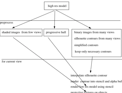
Figure 1: System overview.

its moral equivalent in some form) light field data cannot generally be interpolated or extrapolated very far. When interpolating from a silhouette map, the nearby silhouettes are interpolated in 2D geometrically, and so no ghosting can occur.

When reconstructing new views from a light field/lumigraph representation using geometric correction [35], one obtains a result very similar to view dependent texture mapping. No processing is done on the silhouettes , and so ghosting is still visible on the silhouettes (see Figure 17d of [35]).

Contour Morphing

Contour morphing is an animation technique that creates a smooth transition from one contour to another. Sederberg and Greenwood [38] describe a method that uses a toroidal shortest path approach to solve for a correspondence between points on two simple closed contours. Given such a correspondence, Sederberg et al. [39] use a turtle graphics metaphor to drive the interpolation of intermediate views. Shapira and Rappoport [29] use a star-skeleton decomposition of the contour to achieve higher quality animations. These methods provide no simple way to morph between two contours with differing topologies, and so it would be difficult to use these for silhouette interpolation. Cohen-Or et al. [10] use a distance field interpolation (similar in spirit to [21]) to interpolate between two arbitrary contours. Although this method can handle topology changes and is very useful for animation, for our purposes it would be a rather ad hoc choice. It is not based on the geometry of silhouette generation, has no geometric interpretation, no relation to the visual hull, and will not properly interpolate actual sharp feature points on a silhouette .

(11)

3 System Overview

An overview of our system is described in Figure 1. We begin with a high resolution polyhedral model as input. We first apply a number of preprocessing operations on the data. First we render a small number of views to be later used as textures to projectively map onto the rendered low resolution geometry. We select the views by hand using a simple interactive program. Automatic view selection would be desirable; this remains an open question.

Next a progressive hull construction is run on the high resolution geometry. The resulting progressive hull is a sequence of lower and lower resolution mesh geometries with the property that the volume defined in each successive lower resolution mesh is guaranteed to contain the volume defined by the previous higher resolution meshes. This property allows us to render views of the low resolution geometry which can clipped to a high resolution silhouette .

Finally a silhouette map is constructed. To do this we render binary images of the object as seen from a large number of viewpoints on a surrounding sphere. A pixel-resolution polygonal contour is generated from each image; this contour is then simplified using a simplification algo-rithm similar to [19]. These contours make up a dense silhouette map. We run a silhouette map simplification algorithm to discard views that can be well predicted with the remaining views.

At run time for an arbitrary current view, we find three nearby views on the silhouette map, and an interpolated silhouette is produced. This new silhouette contour is drawn into the stencil buffer. Then the low resolution geometry is rendered using the stencil buffer to clip out the shape of the high resolution silhouette . A subset of the prerendered images are used as projective textures applied to the low res geometry. The result is a rendering with high resolution appearance.

4 Silhouette Map Representation

At the heart of our system is the silhouette map representation. The map represents the shape of the external visible apparent contour (silhouette ) as seen from a number of views. A view

v

istores its

intrinsic and extrinsic camera parameters including the location of the point of viewp

i. The view

also stores the silhouette

s

iseen from that view. The silhouette is represented as a closed polygon,

possibly with holes.

The 3D positions of the optical centers of the view cameras form the vertices of some star shaped triangulated polytope that surrounds the object in question. See plate 6. This polytope is represented as a 3D mesh. The center of the polytopec is also stored in the silhouette map. For

an arbitrary current view pointp

cwe form the segment connecting its position with the center of

the polytope. If the viewpoint lies outside of the polytope, then this segment will intersect the polytope once in the interior of some triangle (or degenerately at some edge or vertex point). If the viewpoint lies inside of the polytope, the segment is extended backwards from the viewpoint until it intersects one of the polytope triangles. There is exactly one intersection because the polytope is star shaped. We call the intersection point on the trianglep

t. The three views

v

1

;v

2

;v

3 stored

(12)

to generate the silhouette for the current view. This triangle intersection pointp

t can be tracked

efficiently as the current view moves continuously by searching the neighborhood of the previous intersection point.

5 Silhouette Interpolation

Given three nearby views

v

1

;v

2

;v

3 (at viewpoints p

1

;

p

2

;

p

3) with their associated silhouettes

s

1

;s

2

;s

3, the goal of silhouette interpolation is to produce a silhouette

s

c for the current view

v

c taken from the viewpoint

p

c. Without 3D information about the silhouettes , this is a difficult

problem and we make a number of approximations to make a solution feasible. In this section we describe our algorithm in detail, and discuss its geometric properties. The algorithm which must be invoked for each rendered frame runs in time

O

triangle) as its viewpoint. In the second step we map

s

tto the current view to produce the current

silhouette

s

c. During this second step we pretend that contour generator for

s

t lies entirely in a

plane that passes through the polytope centercand is parallel to the triangle(p 1

;

p 2

;

p 3 ). 2 It is well known that the image of a planar object undergoes a 2D projective transformation as the view is changed. So we can model this transformation by applying a 3 by 3 matrix to all of the vertices of

s

tto obtain

s

c.

The following pseudocode shows an outline of the entire process. The remainder of this section discusses proceduretriSillInterp().

sill s_c <-- 3dSillInterp(view v_c, sillMap sm){

(p_t, v_1, v_2, v_3) = polytopeIntersection (v_c, sm);

(s_t, v_t) = triSillInterp(p_t, v_1, v_2, v_3, s_1, s_2, s_3); p_1 = v_1.pov; p_2 = v_2.pov; p_3 = v_3.pov;

plane = planeThroughCenter(sm.center, p_1, p_2, p_3); H = determine3by3Matrix(plane, v_t, v_c);

for each vertex index i in s_t s_c[i] = H * s_t[i];

return s_c; }

2

This is an approximation since in general, the contour generator is not a plane curve at all [23]. And nearby points on the external visible apparent contour do not necessarily correspond to nearby points on the contour generator. Moreover, as one moves fromp

tto p

(13)

!!!!!!!!!!!!!!!!!!!!!!!!!!!! !!!!!!!!!!!!!!!!!!!!!!!!!!!! !!!!!!!!!!!!!!!!!!!!!!!!!!!! !!!!!!!!!!!!!!!!!!!!!!!!!!!! !!!!!!!!!!!!!!!!!!!!!!!!!!!! !!!!!!!!!!!!!!!!!!!!!!!!!!!! !!!!!!!!!!!!!!!!!!!!!!!!!!!! !!!!!!!!!!!!!!!!!!!!!!!!!!!! !!!!!!!!!!!!!!!!!!!!!!!!!!!! !!!!!!!!!!!!!!!!!!!!!!!!!!!! !!!!!!!!!!!!!!!!!!!!!!!!!!!! !!!!!!!!!!!!!!!!!!!!!!!!!!!! !!!!!!!!!!!!!!!!!!!!!!!!!!!! !!!!!!!!!!!!!!!!!!!!!!!!!!!! !!!!!!!!!!!!!!!!!!!!!!!!!!!! !!!!!!!!!!!!!!!!!!!!!!!!!!!! !!!!!!!!!!!!!!!!!!!!!!!!!!!! !!!!!!!!!!!!!!!!!!!!!!!!!!!! !!!!!!!!!!!!!!!!!!!!!!!!!!!! !!!!!!!!!!!!!!!!!!!!!!!!!!!! !!!!!!!!!!!!!!!!!!!!!!!!!!!! !!!!!!!!!!!!!!!!!!!!!!!!!!!! !!!!!!!!!!!!!!!!!!!!!!!!!!!! !!!!!!!!!!!!!!!!!!!!!!!!!!!! !!!!!!!!!!!!!!!!!!!!!!!!!!!! !!!!!!!!!!!!!!!!!!!!!!!!!!!!

rectify interpolate rectify

rectify rectify unrectify p1 p2 pe pt original p3 interpolate original original

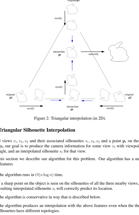
Figure 2: Triangular interpolation (in 2D).

5.1 Triangular Silhouette Interpolation

Given 3 views

v

1

;v

2

;v

3 and their associated silhouettes

s

1

;s

2

;s

3 and a point p t on the triangle p 1

;

p 2

;

p

3 our goal is to produce the camera information for some view

v

t with viewpoint p

t on

the triangle, and an interpolated silhouette

s

tfor that view.

In this section we describe our algorithm for this problem. Our algorithm has a number of unique features

The algorithm runs in

O

(

n

log

n

)time.

If a sharp point on the object is seen on the silhouettes of all the three nearby views, then the

resulting interpolated silhouette

s

twill correctly predict its location. The algorithm is conservative in way that is described below.

The algorithm produces an interpolation with the above features even when the three input

silhouettes have different topologies.

Briefly stated, we solve the triangular silhouette interpolation problem by solving two linear silhouette interpolation subproblems. In the linear silhouette interpolation algorithm we use the

(14)

epipolar geometry of the two views to rectify the two silhouettes , much as in the process of view morphing [37]. The vertices of the two rectified silhouettes are then processed in scan line order. Linear interpolation of the silhouette boundary is performed at the scan lines containing the vertices in order to produce an output set of vertices. Special care must be taken when the two silhouettes have a different number of spans on a given scan line. The resulting vertices are reconnected to create an output silhouette . The details and analysis follow.

Algorithm

Given three silhouettes from three views, finding the actual correspondence between points on these silhouettes is not a well defined problem. This is because as one’s view moves, the points on the contour generator slide locally over the surface. Only at points with infinite curvature (creases) do points on the contour generator remain constant; clearly at these points, the concept of actual correspondence is well defined, and should be obeyed by a silhouette interpolation algorithm. This problem is made even more difficult if the three silhouette polygons have different topologies3

. Thus, barycentric coordinates cannot be directly used.

Given 2 silhouettes from 2 views, there is generally no actual physical correspondence. but there is a “natural” correspondence defined by the epipolar geometry of the two views, which has been used by vision researchers to extract curvature information from silhouettes [7, 14]. We use this epipolar correspondence to create an interpolation algorithm between two views with the desired criteria. Because this epipolar correspondence is only defined for pairs of views, and not triplets of views, we solve for

s

cby solving a sequence of two pairwise interpolation steps.

First we find the edge of the triangle

123 that is closest to p

t. Without loss of generality

suppose this edge is defined by points p 1

;

p

2. We then find the the intersection p

e of that edge

and the line defined byp 3 and

t. See Figure 2. We note that the result of this two-step interpolation

is order-dependent. 4

This is described by the following pseudocode:

(s_t, v_t) <-- triSillInterp(p_t, v_1, v_2, v_3, s_1, s_2, s_3){ p_1 = v_1.pov; p_2 = v_2.pov; p_2 = v_2.pov;

edge_12 = closestEdge((p_t, p_1, p_2, p_3); //wlog p_e = isect(line(p_1,p_2), line(p_t, p_3) ); (s_e, v_e) = linSillInterp(p_e, v_1, v_2, s_1, s_2); (s_t, v_t) = linSillInterp(p_t, v_e, v_3, s_3, s_3);

3

At some singular viewpoints, the topology of the contour generator can change, and new closed contours can be created. At these viewpoints the apparent contour will change its topology. At other singular viewpoints, the topology of the contour generator may remain the same, but the topology of the (projected) apparent contour can change.

4

As we will see below, each stage of linear silhouette interpolation will give us the same silhouette that is predicted by the the visual hull defined by the two input views (for examplevh

12). But the composition of these two steps does

not generate the same silhouette that would be predicted by the visual hull defined by all three viewsvh

123. It is only

(15)

CCCCCCCCCCCCCC CCCCCCCCCCCCCC CCCCCCCCCCCCCC CCCCCCCCCCCCCC CCCCCCCCCCCCCC CCCCCCCCCCCCCC CCCCCCCCCCCCCC CCCCCCCCCCCCCC CCCCCCCCCCCCCC p1 _pe p2 x1l xel x2l l r n f cgl1 α α x1l x2l P1 P2 n f r l x2l x1l

Figure 3: Silhoutette interpolation in an epipolar plane.

return (s_t, v_t); }

5.2 Linear Silhouette Interpolation

Given 2 views

v

1

;v

2 and their associated silhouettes

s

1

;s

2 and a point p e on the edge p 1

;

p 2 our

goal is to produce the camera information for some view

v

ewith viewpoint p

e, and an interpolated

silhouette

s

e for that view.

In this section we describe our algorithm for this problem. In addition to the above features, this step has the following property

If span (defined below) correspondence is solved correctly then

s

e =

sill

(

v

e

;vh

12 )

sill

(

v

e

;vh

1 )

As stated earlier, we wish to use an epipolar geometry to define correspondence. This will allow us to guarantee the above properties. In particular an epipolar decomposition of the scene will allow us to reduce the contour interpolation problem to a set of independent and much easier 1d span interpolation problem restricted to individual scan lines.

Epipolar Decomposition

Epipolar decomposition is most easily accomplished in a rectified domain. Given two silhouettes

s

1

;s

2 taken with 2 views

v

1

;v

2 with locations p

1

;

p

2 we construct the line

l

= p

1

;

p

2. We then

construct two new camera geometries

v

0

;v

0

(16)

and to

l

. We also require that the scan lines of the two image planes are aligned and in correspon-dence. We define the output view

v

e to be a camera with center at

p

0

1 by computing

the appropriate 3 by 3 matrix

H

1and applying it to the silhouette vertices. Likewise for

v

2.

In a rectified context, given some scan line

s

, there is an epipolar plane

ep

s that includes the

scan line

s

and the line

l

joiningp 1

;

p

2. The intersection of

ep

sand a closed 3D surface is generally

a set of closed curves

cr

s. If the epipolar plane intersects the top or bottom of a convex surface

region, then the intersection can include unconnected points called frontier points [2]. See Plate 5. The pin hole projection of the curves

cr

s into the view

v

0

1 will cover a span

sp

1s in scan line

s

. A span is defined by a set of covered intervals; this is described by an even number of vertices. Likewise, the pin hole projection of the curves

cr

sinto the view

v

0 2

will cover a span

sp

2s in scan

v

e. If this can be done for all scan lines

s

, then we have accomplished our

goal. Thus we have reduced a contour interpolation problem to a much easier span interpolation problem.

Algorithm

When the silhouettes are represented as polygons, and the scan line interpolation algorithm per-forms linear interpolation, the output silhouette will be a polygon with vertices at those scan lines where there are vertices in the original silhouettes . As a result, we do not need to apply our span interpolation algorithm at every scan line, but only at the scan lines where there are vertices. The algorithm thus resembles an active edge style polygon scan converter. The vertices of the rectified silhouettes ,

s

0

1

and

s

0 2

, are sorted in

y

order. Scan lines that have vertices are visited from top to bottom. An active edge data structure allows us to quickly determine all of the edge intersects with the scan line. An interpolation is performed on the two spans, which results in an interpolated span. After all of the scan lines are processed, the resulting vertices are connected together to form the output silhouette 5

.

(s_e, v_e) <-- linSillInterp(p_e, v_1, v_2, s_1, s_2){ (v’_1, v’_2) = determineRectification(v_1, v_2); s’_1 = rectify(s_1, v_1, v’_1);

s’_2 = rectify(s_2, v_2, v’_2);

v_e = determineRectifiedEdgeView(p_e, v’_1, v’_2);

sorted = sortVertsByYCoord(s_1,s_2); for each scanline s in sorted{

sp_1s = intersect(s, s_1); //using active edge list sp_2s = intersect(s, s_2); //using active edge list sp_e[s] = spanInterp(v_e, v’_1, v’_2, sp_1s, sp_2s);

5

(17)

}

s_e = connectUpSpans(sp_e); return (s_e, v_e);

}

5.3 Span Interpolation

Given two rectified views

v

0 1

;v

0 2

, with two associated spans

sp

1s

;sp

2s the goal is to interpolate an

output span

sp

esfor the view

v

e. Because we are in a rectified context, this can be viewed entirely

as a rectified problem in flatland(see Figure 3). This makes the problem much easier to analyze and solve.

Single Interval spans

The easiest case to consider (and the most frequent case) is when the epipolar plane

ep

sintersects

the 3D geometry in a single closed curve. In this case, the span seen from each of the two views

v

0 1

;v

0 2

will consist of a single covered interval (see Figure 3). The interval in

v

0 1

is defined by the two image x coordinate numbers

x

1

l;x

1

r

, and the interval in

v

0 2

is defined by the two numbers

x

2

l;x

2

r

.

In this case we use simple linear interpolation to predict the output interval(

xel;xer

).

xel

= (1

)

x

1

l

+(

)

x

2

l

xer

= (1

)

x

1

r

+(

)) corresponds to the

projection of some geometric pointlin space. The pointlmust project in

v

0

1with

x

coordinate

x

1

l

and in

v

0 2

with

x

2

l

. Clearly lmust be the intersection in space between the ray from p

1 passing

through the left of the span on its image plane, and the ray fromp

2 passing through the left of the

span on its image plane, Likewise forr.

The linear interpolation algorithm behaves as if the silhouette was defined by fixed feature pointsl

;

ron the epipolar plane. This of course is not how the actual silhouette would behave on

the curved surface. In the bottom of Figure 3, the dotted curves show the evolution of the actual silhouette while the solid lines show the evolution we predict. The velocity of the actual left point on the contour generatorcgl1as one moves from

v

0 1

to

v

0 2

is governed by the following equation [7]

d

cgl1

d

=( d~r d

~n

)

~r

(1) where

~r

= cgl1 p1 kcgl1 p1k

is the direction from the optical center towards the contour generator,

~n

is the surface normal, and

is the normal curvature (at the pointcgl1) of

cr

, the curve defined by the

(18)

CCCCCCCC CCCCCCCC CCCCCCCC CCCCCCCC CCCCCCCC CCCCCCCC CCCCCCCC CCCCCCCC CCCCCCCC p1 pe p2 Further view l r

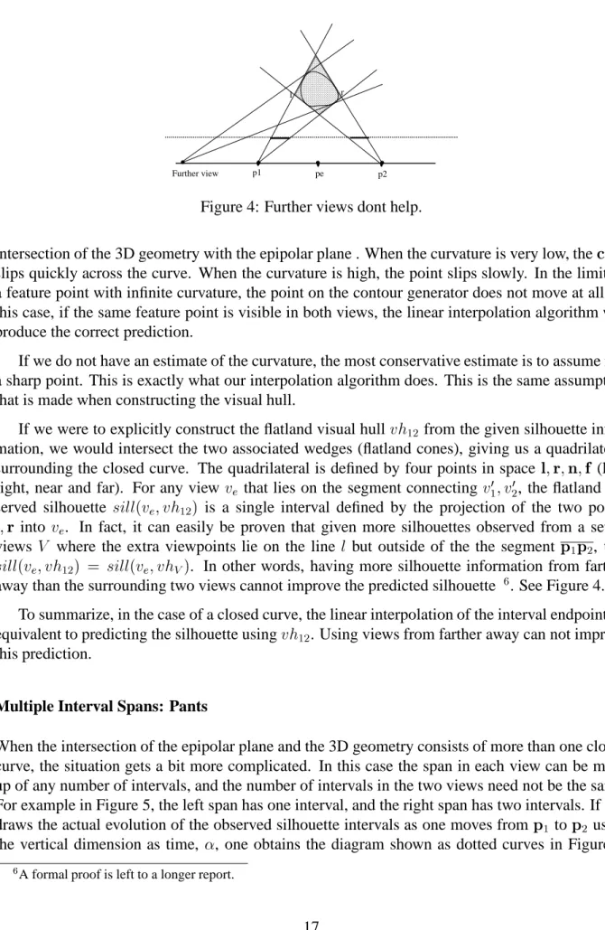
Figure 4: Further views dont help.

intersection of the 3D geometry with the epipolar plane . When the curvature is very low, thecgl1

slips quickly across the curve. When the curvature is high, the point slips slowly. In the limit, at a feature point with infinite curvature, the point on the contour generator does not move at all. In this case, if the same feature point is visible in both views, the linear interpolation algorithm will produce the correct prediction.

If we do not have an estimate of the curvature, the most conservative estimate is to assume it is a sharp point. This is exactly what our interpolation algorithm does. This is the same assumption that is made when constructing the visual hull.

If we were to explicitly construct the flatland visual hull

vh

e

;vh

12 ) =

sill

(

v

e

;vh

V

). In other words, having more silhouette information from farther

away than the surrounding two views cannot improve the predicted silhouette 6

. See Figure 4. To summarize, in the case of a closed curve, the linear interpolation of the interval endpoints is equivalent to predicting the silhouette using

vh

12. Using views from farther away can not improve

this prediction.

Multiple Interval Spans: Pants

When the intersection of the epipolar plane and the 3D geometry consists of more than one closed curve, the situation gets a bit more complicated. In this case the span in each view can be made up of any number of intervals, and the number of intervals in the two views need not be the same. For example in Figure 5, the left span has one interval, and the right span has two intervals. If one draws the actual evolution of the observed silhouette intervals as one moves fromp

1 to p

2 using

the vertical dimension as time,

, one obtains the diagram shown as dotted curves in Figure 5.

6

(19)

CCCCCCCCCCCCCC CCCCCCCCCCCCCC CCCCCCCCCCCCCC CCCCCCCCCCCCCC CCCCCCCCCCCCCC CCCCCCCCCCCCCC CCCCCCCCCCCCCC CCCCCCCCCCCCCC CCCCCCCCCCCCCC CCCCCCCCCCCCCC CCCCCCCCCCCCCC p1 p2 CCCCCCCCCCCC CCCCCCCCCCCC CCCCCCCCCCCC CCCCCCCCCCCC CCCCCCCCCCCC CCCCCCCCCCCC CCCCCCCCCCCC α Figure 5: Pants.

Clearly this exact shape would be hard to predict simply from the silhouette information in the two views.

2

lb;x

2

rb

one performs the following pants computation

xela = lerp(alpha, x1l, x2la); xera = lerp(alpha, x1r, x2ra); xelb = lerp(alpha, x1l, x2lb); xerb = lerp(alpha, x1r, x2rb); if (xelb < xera)

return (xela, xerb); else

return (xela, xera, xelb, xerb);

In the case

xelb < xera

the image of the two quadrilaterals in

vh

12overlap in the output view, and

only one interval is output. Otherwise, the image includes 2 intervals which are output. In either case, the correct visual hull is reproduced.

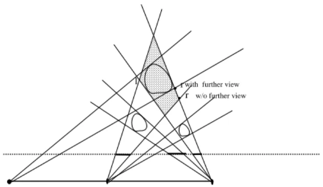
We note that in the case of multiple intervals, it is not the case that one will not be helped by silhouette information from farther views, i.e.,

sill

(

v

e

;vh

12

) 6=

sill

(

v

e

;vh

V

). For example

(20)

CCCCCCC CCCCCCC CCCCCCC CCCCCCC CCCCCCC CCCCCCC CCCCCCC CCCCCCC CCCCCCC CCCCCCC CCCCCCC p1 p2 Further view

w/o further view with further view

l

r r

Figure 6: Further views do help. prediction may be suboptimal.

Mutant Pants

The pants algorithm can be extended in a straightforward manner to include more complicated topological changes such as n-legged pants, and two-sided-no-torso pants (see Figure 8).

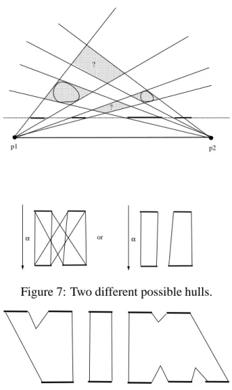
In Figure 7, we show an example where both the left and right views have spans with two intervals. The visual hull here is defined by the four shaded quadrilaterals, which results in two sided pants. If there is no geometry in the front and back quadrilaterals, then this is overly conser-vative. If we can determine that during the interpolation, the two observed silhouette intervals do not interact, then we can use the less conservative interpolation shown on the right. More generally given

n

intervals for

v

0

1, and

m

intervals for

v

0

2, we attempt to group the intervals in into cliques

such as those shown in in Figure 8. An independent pants is created for each clique.

We have developed a heuristic algorithm for clique determination using the matching of frontier points and tracking from span to span. Stated briefly, for the pair of views, we attempt to form a correspondence between the convex and concave minima and maxima of the silhouette . Matched extrema, and their associated spans are put in separate cliques. Unmatched extrema and their associated spans are put in the nearest existing clique. This heuristic works well if the views are taken closely together with few topological changes between the views. An adequate sampling rate is set adaptively by the silhouette map simplification algorithm described next.

6 Silhouette Map Simplification

In a silhouette map, views are sampled at a set of vertices describing a star-shaped polytope sur-rounding the object. For most objects, a uniform sampling is inefficient. In some regions of view space, the silhouette changes slowly (for example

in equation 1 may be large). In other regions, the silhouette may change rapidly. Geometrically this can occur where

k

is small. Moreover when topological changes occur, our interpolation algorithm uses the pants connection, which can be

(21)

CCCCCCCCC CCCCCCCCC CCCCCCCCC CCCCCCCCC CCCCCCCCCCC CCCCCCCCCCC CCCCCCCCCCC CCCCCCCCCCC CCCCCCCCCCC CCCCCCCCCCC CCCCCCCCCCC CCCCCCCCCCC p1 p2 α ? or α ? CCCCCCCCCC CCCCCCCCCC CCCCCCCCCC CCCCCCCCCC CCCCCCCCCC CCCCCCCCCC CCCCCCC CCCCCCC CCCCCCC CCCCCCC CCCCCCC

Figure 7: Two different possible hulls.

Figure 8: Cliques with mutant pants.

quite conservative, making a higher sampling rate desirable. Our solution to this is to use an adap-tive sampling in the silhouette map. This is achieved using a greedy silhouette map simplification procedure that is inspired by the mesh simplification algorithm described in [19].

In particular, we begin with a silhouette map that contains many samples, densely surrounding the object. It is this original data that any simplified map must approximate. During the simpli-fication process, any edge on the silhouette map polytope can be collapsed and one of its views discarded. We associate with each edge the error that would be incurred by collapsing it. The error is measured by comparing the original silhouette data points with predictions that would be made by the simplified mesh. The error metric measures the number of pixels that are misclassified (interior/exterior) by the prediction. Since we wish the polytope to remain star shaped, an edge is given infinite cost if its collapse would lead to a non-star shape.

The edges are stored in a heap, sorted by cost. The lowest cost edge is removed from the heap, and is collapsed in the silhouette map. The edges in the neighborhood of the collapse must then have their costs reevaluated.

(22)

consuming, and is run as a preprocess.

7 Construction of progressive hulls

For the rendering application in this paper, we need to compute, for an arbitrary triangle mesh

M

n

, a set of one or more coarser approximating meshes that completely enclose

M

n

. In this section, we solve the somewhat more general problem of constructing from

M

n

n )

n

. Before presenting the technique in more detail, let us first more precisely defineV(

M

).

Definition of interior volume The given mesh

M

n

is assumed to be orientable and closed (i.e. it has no boundaries). The mesh may have several connected components, and may contain interior cavities (e.g. a hollowed sphere). In most cases, it is relatively clear which points lie in the interior volumeV(

M

). The definition of interior is less obvious in the presence of self-intersections, or

when surfaces are nested (e.g. concentric spheres). Interfaces for 2D rasterization often allow several rules to define the interior of non-simple polygons [1, 32]. These rules do generalize to the case of meshes in 3D, as shown next.

To determine if a point p 2 R 3

lies in the interior of a mesh

M

, select a ray from p off to

M

(p)6=0. With the even-odd rule, the condition is that

w

M

(p)is odd. In this work, we use the positive winding rule which defines interior volume as V(

M

)=fp 2R

3 :

w

M

(p)

>

0g

:

Progressive mesh representation The progressive hull (PH) sequence is an adaptation of the earlier progressive mesh (PM) representation [19] developed for level-of-detail control and pro-gressive transmission of geometry.

The PM representation of a mesh

M

n

is obtained by simplifying the mesh through a sequence of edge collapse transformations, and recording their inverses. Specifically, the PM representation consists of a coarse base mesh

M

0

(23)

v

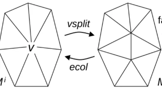
vsplit ecol Mi _Mi+1 faces Fi faces Fi+1

Figure 9: The vertex split transformation and its inverse, the edge collapse transformation. progressively recover detail. Thus, the representation captures a continuous family of approximat-ing meshes

M

0

:::M

n

.

As shown in Figure 9, each edge collapse transformation unifies two adjacent vertices into one, thereby removing two faces from the mesh. For the purpose of level-of-detail control, edge collapses are selected so as to best preserve the appearance of the mesh during simplification. Several appearance metrics have been developed (e.g. [9, 13, 17, 19, 26]).

In this paper, we show that proper constraints on the selection of edge collapse transformations allow the creation of PM sequences that are progressive hulls.

Progressive hull construction For the PM sequence to be a progressive hull, each edge collapse transformation

M

i+1

!

M

i

must satisfy the property

V(

M

i

)V(

M

i+1

)

:

A sufficient condition is to guarantee that, at all points in space, the winding number either remains constant or increases: 8p2R 3

; w

M i+1(p)

w

M i(p)

:

Intuitively, the surface must either remain unchanged or locally move “outwards” everywhere. Let

F

i

and

F

i+1

denote the sets of faces in the neighborhood of the edge collapse as shown in Figure 9, and let v be the position of the unified vertex in

M

i

The position v is found with a linear programming algorithm, using the above linear

in-equality constraints and the goal function of minimizing volume. Mesh volume, defined here

7

We currently hypothesize that preventing self-intersections inF i

andF i+1

(24)

as

R p2R

3

w

M

(p)

d

p, is a linear function onvthat involves the ring of vertices adjacent tov(refer

to [17, 26]).

n

, and for each edge collapse

M

i+1 !

0

:::

M

n

. By simply reversing the orientation of the initial mesh

M

n

, the same construction gives rise to an progressive inner hull sequence

M

0

:::

M

n

. Combining these produces a single sequence of hulls

M

0

:::

M

n =

M

n

:::

M

0

that bounds the mesh

M

n

from both sides.

We expect that this representation will also find useful applications in collision detection, par-ticularly using a selective refinement framework [20, 42].

8 Rendering Using Silhouette Clipping

To exploit the computed polygonal silhouette, we structure the rendering process as follows. First, we draw the silhouette polygon into the stencil plane of the frame buffer, setting the stencil bits at each pixel such that future rendering operations only affect the interior of the silhouette polygon. Second, we render the coarse mesh subject to the stencil, mapping textures onto the mesh faces using the precomputed object views. Finally, to obtain an anti-aliased silhouette, we render the silhouette polygon as an anti-aliased polyline, recording the alpha values in the frame buffer. We then render the coarse mesh again, using those computed alpha values at the silhouette pixels. We next describe each of these steps in further detail.

(25)

8.1 Silhouette clipping

At each frame, the stencil plane is initialized to zero as part of the frame buffer clear operation. Even though the silhouette polygon is generally concave and contains holes, it can be rasterized into the stencil plane efficiently as a single triangle fan. The trick is to use parity bits so that overlapping triangles cancel out correctly; for details, refer to the OpenGL programming guide [33]. Note that drawing the silhouette polygon is a simple 2D rasterization operation and is thus extremely fast. Having established the silhouette in the stencil plane, we next render the coarse mesh subject to the stencil.

8.2 Projective textures

In a precomputation stage, we store a small number of shaded images of the high resolution ge-ometry as textures. For each face of the coarse mesh, we compute the set of texture views from which it is completely visible [12]. This set of visible textures is stored as a visibility bit vector associated with the face.

During rendering we sort the texture views in order of increasing distance from the current camera view, where distance is simply Euclidean distance between the camera centers. The number of texture views is generally small (e.g. 20) so this sorting operation is fast. For each face of the coarse mesh, the texture used to texture map the face is taken to be the closest texture view that is contained in the visibility bit vector.

At each vertex of the face, the projective texture coordinates are obtained by projecting a 3D position into the appropriate texture view. While we could simply use the position of the ver-tex, texture map distortion is reduced by instead using the parametrizations P(v) computed in

Section 7.

8.3 Anti-aliasing of the silhouette

One benefit of the silhouette clipping approach is that the silhouette can be anti-aliased even if the hardware lacks polygonal anti-aliasing. To achieve this, the silhouette polygon is rendered again simply as a 2D anti-aliased polyline, but only affecting the alpha channel of the frame buffer. Then, the mesh is rendered, using the alpha values already in framebuffer.

As with conventional polygonal rendering, correct anti-aliasing in the presence of multiple objects requires that the objects be rendered in back-to-front order.

9 Results

Plate 1 shows meshes in a progressive hull sequence for a mesh of69

;

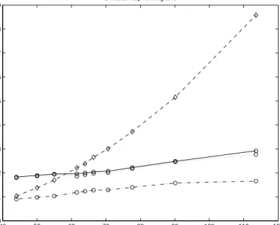
674 faces. Construction of

(26)

40 50 60 70 80 90 100 110 120 0 0.01 0.02 0.03 0.04 0.05 0.06 0.07 0.08 0.09

number of vertices on silhoutte

execution time per frame (s)

silhoutte map running time

Figure 10: Rendering speeds. speed. Plate 2 shows another example.

Figure 2 shows an example of silhouette interpolation. Note that the resulting silhouette has a different topology than any of the original data.

Plate 3 shows silhouette clipping used for efficient high quality rendering. In (a) the original high resolution mesh is shown. In (b) we show a low resolution approximation with 500 faces. In (c) the low resolution geometry is texture mapped using 20 precomputed texture views. In (d) we show the interpolated silhouette for this view. In (e), the interpolated silhouette is used to clip the low resolution mesh. In (f) the silhouette is also used to antialias the silhouette of the low resolution geometry.

In figure 10 we show timing performance on an SGI R5K, of our algorithm on the bunny data set. For the low resolution geometry we use 500 faces. The horizontal axis measures

n

, the (average) number of vertices in each of the silhouette contours of the silhouette map. The dot-dash line shows the time it takes to perform the silhouette interpolation for each frame. The dotted line shows the time it takes to interpolate the silhouette , and draw the low resolution using silhouette clipping. The solid line shows the time to interpolate, silhouette clip and apply projective textures. For comparison, we show timings for rendering high resolution geometry with

n

2

faces. For evenly tessellated objects, it takes roughly

n

2

faces to obtain a silhouette with

n

vertices. This is shown with a dashed line.

Plate 6 shows an example of our silhouette map simplification algorithm. We begin with 1024 evenly spaced views about the torus. When we have reached 128 views, the structure of the re-maining star shaped polytope appears to be well tuned to the structure of silhouette changes for various directions.

(27)

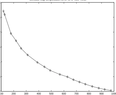
100 200 300 400 500 600 700 800 900 1000 0 0.005 0.01 0.015 0.02 0.025 0.03 number of views average error

Silhoutte Map Simplification Error for 3−hole Torus

Figure 11: Silhouette map simplification error.

In figure 11, we show the performance of our simplification algorithm on the torus data set. The horizontal axis measures the number of views kept. Error is measured by comparing the original 1024 silhouette contours to those predicted by the simplified map. The number of misclassified pixels (exterior/interior) is measured. This number is divided by the entire number of pixels in the interior of the object for that view. This is summed up over all the views and divided by 1024. The simplification algorithm in conjunction with the silhouette interpolation method described produces a silhouette map with high fidelity and minimal storage overhead.

10 Discussion

We have introduced the framework of silhouette clipping, in which low-resolution geometry is ren-dered and clipped to a more accurate silhouette. During a preprocess, a silhouette map is formed by sampling the object silhouette from a discrete set of viewpoints. Interpolation of these silhouettes was made principled using a visual hull approximation of the model in a rectified epipolar setting. Topological changes between adjacent silhouettes can be handled properly by this algorithm. We reduced storage of the silhouette map through adaptive simplification.

To guarantee that the geometry be at least as large as the silhouette, we presented a technique for constructing a nested sequence of meshes, in which each coarser mesh completely encloses the original mesh.

(28)

Acknowledgements

We would like to thank Aaron Isaksen for help with the Faro Arm, Peter-Pike Sloan for helpful input, and Julie Dorsey for making the MIT LCS graphics lab available to us. This work has been supported in part by NSF Career Awards 9703399, A Sloan research fellowship, and an IBM partnership award.

References

[1] ADOBESYSTEMSINC. Postscript Language Reference Manual, second ed. Addison Wesley, 1990.

[2] B.VIJAYAKUMAR,D.KRIEBMAN,AND J.PONCE. structure and motion of curved 3d objects from moncular silhouettes. Proc CVPR 96.

[3] BAJAJ, C., ANDSCHIKORE, D. Error-bounded reduction of triangle meshes with

multivari-ate data. SPIE 2656 (1996), 34–45.

[4] BLYTHE, D., GRANTHAM, B., NELSON, S., AND MCREYNOLDS, T. advanced graphics

programming techniques using opengl.

[5] BOYER, E., AND BERGER, M. 3d surface reconstruction using occluding contours. IJCV

22, 3 (1997), 219–233.

[6] CIGNONI, P., MONTANI, C., ROCCHINI, C., AND SCOPIGNO, R. A general method for preserving attribute values on simplified meshes. In Visualization ’98 Proceedings (1998), IEEE, pp. 59–66.

[7] CIPOLLA, R., AND BLAKE, A. surface shape from the deformation of apparent contours.

IJCV 9, 2 (1992), 83–112.

[8] COHEN, J., MANOCHA, D.,AND OLANO, M. Simplifying polygonal models using

succes-sive mappings. In Visualization ’97 Proceedings (1997), IEEE, pp. 81–88.

[9] COHEN, J., OLANO, M.,ANDMANOCHA, D. Appearance-preserving simplification.

Com-puter Graphics (SIGGRAPH ’98 Proceedings) (1998), 115–122.

[10] DANIEL COHEN OR,DAVID LEVIN,AND AMIRA SOLOMOVICI. contour blending using warp

guided distance field interpolation. proc visualization 96, 165–172.

[11] DEBEVEC, P., C.TAYLOR, AND J. MALIK. modeling and rendering architecture from

pho-tographs. SIGGRAPH 96, 11–20.

[12] DEBEVEC, P.,Y.YU,AND G.BORSHUKOV. efficient view dependent image based rendering