Turning Big data into tiny data:
Constant-size coresets for
k
-means, PCA and projective clustering
Dan Feldman
∗Melanie Schmidt
†Christian Sohler
†Abstract
We prove that the sum of the squared Euclidean distances from thenrows of ann×dmatrixAto any compact set that is spanned by k vectors in Rd can
be approximated up to (1 +ε)-factor, for an arbitrary smallε >0, using theO(k/ε2)-rank approximation of
Aand a constant. This implies, for example, that the optimalk-means clustering of the rows ofAis (1 +ε )-approximated by an optimal k-means clustering of their projection on the O(k/ε2) first right singular
vectors (principle components) ofA.
A (j, k)-coreset for projective clustering is a small set of points that yields a (1 +ε)-approximation to the sum of squared distances from the n rows of A toany set ofkaffine subspaces, each of dimension at most j. Our embedding yields (0, k)-coresets of size O(k) for handlingk-means queries, (j,1)-coresets of size O(j) for PCA queries, and (j, k)-coresets of size (logn)O(jk)for anyj, k≥1 and constantε∈(0,1/2).
Previous coresets usually have a size which is linearly or even exponentially dependent of d, which makes them useless whend∼n.
Using our coresets with the merge-and-reduce ap-proach, we obtain embarrassingly parallel streaming algorithms for problems such as k-means, PCA and projective clustering. These algorithms use update time per point and memory that is polynomial in logn and only linear ind.
For cost functions other than squared Euclidean distances we suggest a simple recursive coreset con-struction that produces coresets of size k1/εO(1)
for k-means and a special class of bregman divergences that is less dependent on the properties of the squared Euclidean distance.
∗MIT, Distributed Robotics Lab. Email: dan-nyf@csail.mit.edu
†TU Dortmund, Germany, Email: {melanie.schmidt,
1 Introduction
Big Data. Scientists regularly encounter limitations due to large data sets in many areas. Data sets grow in size because they are increasingly being gathered by ubiquitous information-sensing mobile devices, aerial sensory technologies (remote sensing), genome sequencing, cameras, microphones, radio-frequency identification chips, finance (such as stocks) logs, internet search, and wireless sensor networks [30, 38]. The world’s technological per-capita capacity to store information has roughly doubled every 40 months since the 1980s [31]; as of 2012, every day 2.5 etabytes(2.5×10¹⁸) of data were created [4]. Data
sets as the ones described above and the challenges involved when analyzing them is often subsumed in the termBig Data.
Gartner, and now much of the industry use the “3Vs” model for describing Big Data [14]: increasing volume n(amount of data), itsvelocity (update time per new observation) and its variety d (dimension, or range of sources). The main contribution of this paper is that it deals with cases where bothnandd are huge, and does not assumed≪n.
Data analysis. Classical techniques to analyze and/or summarize data sets include clustering, i.e. the partitioning of data into subsets of similar char-acteristics, and dimension reduction which allows to consider the dimensions of a data set that have the highest variance. In this paper we mainly consider problems that minimize the sum of squared error, i.e. we try to find a set of geometric centers (points, lines or subspaces), such that the sum of squared distances from every input point to its nearest center is mini-mized.
Examples are thek-meansor sum of squares clus-tering problem where the centers are points. An-other example is thej-subspace meanproblem, where k = 1 and the center is a j-subspace, i. e., the sum of squared distances to the points is minimized over allj-subspaces. The j-rank approximation of a ma-trix is the projection of its rows on theirj-subspace mean. Principal component analysis (PCA) is an-other example where k = 1, and the center is an
affine subspace. Constrained versions of this prob-lem (that are usually NP-hard) include the non-negative matrix factorization (NNMF) [2], when the j-subspace should be spanned by positive vectors, and Latent Dirichlet Allocation (LDA) [3] which general-izes NNMF by assuming a more general prior distri-bution that defines the probability for every possible subspace.
The most general version of the problem that we study is the linear or affine j-Subspace k-Clustering problem, where the centers are j-dimensional linear or affine subspaces and k≥1 is arbitrary.
In the context of Big Data it is of high interest to find methods to reduce the size of the streaming data but keep its main characteristics according to these optimization problems.
Coresets. A small set of points that approximately maintains the properties of the original point with respect to a certain problem is called a coreset (or core-set). Coresets are a data reduction technique, which means that they tackle the first two ‘Vs’ of Big Data, volumenand velocity (update time), for a large family of problems in machine learning and statistics. Intuitively, a coreset is a semantic compression of a given data set. The approximation is with respect to a given (usually infinite) set Qof query shapes: for every shape in Qthe sum of squared distances from the original data and the coreset is approximately the same. Running optimization algorithms on the small coreset instead of the original data allows us to compute the optimal query much faster, under different constraints and definition of optimality.
Coresets are usually of size at most logarithmic in the number n of observations, and have similar update time per point. However, they do not handle the variety of sourcesdin the sense that their size is linear or even exponential ind. In particular, existing coreset are useless for dealing with Big Data when d ∼ n. In this paper we suggest coresets of size independent ofd, while still independent or at most logarithmic in n.
Non-SQL databases. Big data is difficult to work with using relational databases of n records in d columns. Instead, in NOSQL is a broad class of database management systems identified by its non-adherence to the widely used relational database management system model. In NoSQL, every point in the input stream consists of tuples (object, feature, value), such as (”Scott”, ”age”, 25). More generally, the tuple can be decoded as (i, j, value) which means that the entry of the input matrix in theith row and jth column isvalue. In particular, the total number of observations and dimensions (nandd) is unknown
while passing over the streaming data. Our paper support this non-relational model in the sense that, unlike most of previous results, we do not assume that eitherdornare bounded or known in advance. We only assume that the first coordinates (i, j) are increasing for every new inserted value.
2 Related work
Coresets. The term coreset was coined by Agarwal, Har-Peled and Varadarajan [10] in the context of extend measures of point sets. They proved that every point set P contains a small subset of points such that for any direction, the directional width of the point set will be approximated. They used their result to obtain kinetic and streaming algorithms to approximately maintain extend measures of point sets.
Application to Big Data. An off-line coreset construction can immediately turned into streaming and embarrassingly parallel algorithms that use small amount of memory and update time. This is done using a merge-and-reduce technique as explained in Section 10. This technique makes coresets a practi-cal and provably accurate tool for handling Big data. The technique goes back to the work of Bentley and Saxe [11] and has been first applied to turn core-set constructions into streaming algorithms in [10]. Popular implementations of this technique include Hadoop [40].
Coresets for k-points clustering (j = 0). The first coreset construction for clustering problems was done by Badoiu, Har-Peled and Indyk [13], who showed that fork-center,k-median andk-means clus-tering, an approximate solution has a small witness set (a subset of the input points) that can be used to generate the solution. This way, they obtained im-proved clustering algorithms. Har-Peled and Mazum-dar [29] gave a stronger definition of coresets fork -median andk-means clustering. Given a point setP this definition requires that forany setofkcentersC the cost of the weighted coresetSwith respect toP is approximated upto a factor of (1 +ε). Here,Sis not necessarily a subset ofP. We refer to their definition as astrong coreset.
Har-Peled and Kushal [28] showed strong coresets for low-dimensional space, of size independent of the number of input points n. Frahling and Sohler designed a strong coreset that allows to efficiently maintain a coreset for k-means in dynamic data streams [24]. The first construction of a strong coreset fork-median and k-means of size polynomial in the dimension was done by Chen [15]. Langberg and Schulman [35] defined the notion ofsensitivity of an
input point, and used it to construct strong coresets of size O(k2d2/ε2), i.e, independent ofn. Feldman and
Langberg [21] showed that small total sensitivity and VC-dimension for a family of shapes yields a small coreset, and provided strong coresets of sizeO(kd/ε2)
for thek-median problem.
Feldman, Monemizadeh and Sohler [22] gave a construction of a weak coreset of size independent of both the number of input pointsnand the dimension d. The disadvantage of weak coresets is that, unlike the result in this paper, they only give a guarantee for centers coming from a certain set of candidates (instead of any set of centers as in the case of strong coresets).
Feldman and Schulman [23] developed a strong coreset for thek-median problem when the centers are weighted, and for generalized distance functions that handle outliers. There are also efficient implemen-tation ofk-means approximation algorithm based on coresets, both in the streaming [9] and non-streaming setting [25].
j-subspace clustering (k= 1). Coresets have also been developed for the subspace clustering problem. The j-dimensional subspace of Rd that minimizes
the sum of squared distances to n input points can be computed in O(min
nd2, dn2 ) time using the
Singular Value Decomposition (SVD). The affine j -dimensional subspace (i.e, flat that does not intersect the origin) that minimizes this sum can be computed similarly using principle component analysis (PCA), which is the SVD technique applied after translating the origin of the input points to their mean.
In both cases, the solution for the higher di-mensional (j + 1)-(affine)-subspace clustering prob-lem can be obtained by extending the solution to the j-(affine)-subspace clustering problem by one dimen-sion. This implicitely defines an orthogonal basis of
Rd. The vectors of these bases are calledright
singu-lar vectors, for the subspace case, andprinciple com-ponents for the affine case.
A line of research developed weak coresets for faster approximations [16, 17, 39, 26]. These results are usually based on the idea to sample sets of points with probability roughly proportional to the volume of the simplex spanned by the points, because such a simplex will typically have a large extension in the directions defined by the first left singular vectors. See recent survery in [8] for weak coresets.
Feldman, Fiat and Sharir [19] developed a strong coreset for the subspace approximation problem in low dimensional spaces, and Feldman, Monemizadeh, Sohler and Woodruff [20] provided such a coreset for high dimensional spaces that is polynomial in the dimension of the input space d and exponential in
the considered subspace j. Feldman and Langberg [21] gave a strong coreset whose size is polynomial in bothdand j.
Constrained optimization (e.g. NNMF, LDA). Non-negative matrix factorization (NNMF) [2], and Latent Dirichlet Allocation (LDA) [3] are constrained versions of thej-subspace problem. In NNMF the de-siredj-subspace should be spanned by positive vec-tors, and LDA is a generalization of NNMF, where we are given additinal prior probabilities (e.g., mul-tiplicative cost) for every candidate solution. An im-portant practical advantage of coresets (unlike weak coresets) is that they can be used with existing al-gorithms and heuristics for such constrained opti-mization problems. The reason is that strong core-set approximates the sum of squared distances toany given shape from a family of shapes (in this case,j -subspaces), independently for a specific optimization problem. In particular, running heuristics for a con-strained optimization problem on anε-coreset would yield the same quality of approximations compared to such run on the original input, up to provable (1 +ε )-approximation. While NNMF and LDA are NP-hard, coresets forj-subspaces can be constructed in poly-nomial (and usually practical) time.
k-lines clustering (j = 1). For k-lines clustering, Feldman, Fiat and Sharir [19] show strong coresets for low-dimensional space, and [21] improve the result for high-dimensional space. In [23] the size of the coreset reduced to be polynomial in 2O(k)logn. Har-Peled
proved a lower bound of min
2k,logn for the size
of such coresets.
Projective clustering (k, j > 1). For general projective clustering, where k, j ≥ 1, Har-Peled [27] showed that there is no strong coreset of size sub-linear inn, even for the family of pair of planes inR3
(j = k = 2, d = 3). However, recently Varadarajan and Xiao [36] showed that there is such a coreset if the input points are on an integer grid whose side length is polynomial inn.
Bregman divergences. Bregman divergences are a class of distance measures that are used frequently in machine learning and they includel2
2. Banerjee et
al. [12] generalize the Lloyd’s algorithm to Bregman divergences for clustering points (j= 0). In general, Bregman divergences have singularities at which the cost might go to infinity. Therefore, researchers studied clustering for so-called µ-similar Bregman divergences, where there is an upper and lower bound by constant µ times a Mahalanobis distance [7]. The only known coreset construction for clustering under Bregman divergences is a weak coreset of
size O(klogn/ε2log(|Γ|klogn)) by Ackermann and
Bl¨omer [6].
3 Background and Notation
We deal with clustering problems on point sets in Euclidean space, where a point set is represented by the rows of a matrixA. The input matrixAand all other matrices in this paper are over the reals. Notations and Assumptions. The number of input points is denoted by n. For simplicity of notation, we assume that d = n and thus A is an n×nmatrix. Otherwise, we add (n−d) columns (or d−nrows) containing all zeros to A. We label the entries ofAbyai,j. Theith row ofAwill be denoted
as Ai∗ and thejth columns asA∗j.
The identity matrix ofRjis denoted asI∈Rj×j.
For a matrix X with entries xi,j, we denote the
Frobenius norm ofX bykXk2=
q P
i,jx2i,j. We say
that a matrix X ∈ Rn×j has orthonormal columns
if its columns are orthogonal unit vectors. Such a matrix is also called orthogonal matrix. Notice that every orthogonal matrixX satisfiesXTX=I.
The columns of a matrix X span a linear sub-space L if all points in L can be written as linear combinations of the columns ofA. This implies that the columns contain a basis ofL.
A j-dimensional linear subspace L ⊆ Rn will
be represented by an n ×j basis matrix X with orthonormal columns that span L. The projection of a point set (matrix) A on a linear subspace L represented by X will be the matrix (point set) AX ∈ Rn×j. These coordinates are with respect to
the column space of X. The projections of A on L using the coordinates ofRn are the rows of AXXT.
Distances to Subspaces. We will often compute the squared Euclidean distance of a point set given as a matrix A to a linear subspace L. This distance is given bykAYk2
2, whereY is ann×(n−j) matrix with
orthonormal columns that span L⊥, the orthogonal complement of L. Therefore, we will also sometimes represent a linear subspaceLby such a matrixY.
An affine subspace is a translation of a linear subspace and as such can be written asp+L, where p ∈ Rn is the translation vector and L is a linear
subspace.
For a compact setS ⊆Rd and a vector pin Rd,
we denote the Euclidean distance between pand (its closest points in)S by
dist2(p, S) := min
s∈Skp−sk 2 2.
For an n×dmatrixAwhose rows arep1,· · ·, pn, we
define the sum of the squared distances fromA to S by (3.1) dist2(A, S) = n X i=1 dist2(pi, S).
Thus, if L is a linear j-subspace and Y is a matrix with n− j orthonormal columns spanning L⊥, then dist(p, L) = kpTYk
2. We generalize the
notation to n×n matrices and define, dist(A, L) =
Pn
i=1dist(Ai∗, L) for any compact setL. HereAi∗ is
theith row ofA. Furthermore, we write dist2(A, L) =
Pn
i=1 dist(Ai∗, L)
2
.
Definition 1. (Linear (Affine) j-Subspace k -Clustering)Given a set of npoints inn-dimensional space as an n × n matrix A, the k j-subspace clustering problem is to find a set L of k linear (affine) j-dimensional subspaces L1, . . . , Lk of Rd
that minimizes the sum of squared distances to the nearest subspace, i.e.,
cost(A, L) = n X i=1 min j=1...,kdist 2 (Ai∗, Lj)
is minimized over every choice ofL1,· · ·, Lk.
Singular Value Decomposition. An important tool from linear algebra that we will use in this paper is the singular value decomposition of a matrix A. Recall that A = U DVT is the Singular Value
Decomposition (SVD) of A if U, V ∈ Rn×n are
orthogonal matrices, and D ∈ Rn×n is a diagonal
matrix with non-increasing entries. Let (s1,· · ·, sn)
denote the diagonal ofD2.
For an integer j between 0 to n, the first j columns ofV span a linear subspaceL∗that minimize the sum of squared distances to the points (rows) of A, over allj-dimensional linear subspaces inRn. This
sum equalssj+1+. . .+sn, i.e. for anyn×(n−j)
matrixY with orthonormal columns, we have
(3.2) kAYk2 2≥ n X i=j+1 si.
The projection of the points ofAonL∗ are the rows of U D. The sum of the squared projection of the points ofAonL∗iss
1+. . .+sj. Note that the sum
of squared distances to the origin (the optimal and only 0-subspace) iss1+. . .+sn.
Coresets. In this paper we introduce a new notion of coresets, which is a small modification of the earlier definition by Har-Peled and Mazumdar [29] for thek-median andk-means problem (here adapted to the more general setting of subspace clustering)
that is commonly used in coreset constructions for these problems. The new idea is to allow to add a constant C to the cost of the coreset. Interestingly, this simple modification allows us to obtain improved coreset constructions.
Definition 2. Let Abe ann×dmatrix whose rows represents n points in Rd. An m ×n matrix M
is called (k, ε)-coreset for thej-subspace k-clustering problem of A, if there is a constant c such that for every choice of k j-dimensional subspaces L1, . . . , Lk
we have
(1−ε) cost(A, L)≤cost(M, L)+c≤(1+ε) cost(A, L). 4 Our results
In this section we summarize our results.
The main technical result is a proof that the sum of squared distances from a set of points inRd (rows
of an n ×d matrix A) to any other compact set that is spanned by k vectors of Rd can be (1 +ε
)-approximated using the O(k/ε)-rank approximation of A, together with a constant that depends only on A. Here, a distance between a pointpto a set is the Euclidean distance ofpto the closest point in this set. TheO(k/ε)-rank approximation ofAis the projection of the rows of Aon thek-dimensional subspace that minimizes their sum of squared distances. Hence, we prove that the low rank approximation of A can be considered as a coreset for its n rows. While the coreset also has n rows, its dimensionality is independent ofd, but only onkand the desired error. Formally:
Theorem 4.1. Let A be an n×d matrix, k ≥1 be an integer and 0 < ε < 1. Suppose that Am is the
m-rank approximation of A, where m:=b⌈k/ε2≤n
for a sufficiently large constant b. Then for every compact set S that is contained in a k-dimensional subspace of Rd, we have
(1−ε)dist2(A, S)≤dist2(Am, S) +kA−Amk2
≤(1 +ε)dist2(A, S),
wheredist2(A, S)is the sum of squared distances from each row on Ato its closest point in S.
Note that A takes nd space, while the pair Am
and the constantkA−Amkcan be stored usingnm+1
space.
Coresets. Combining our main theorem with known results [21, 19, 36] we gain the following coresets for projective clustering. All the coresets can handle Big data (streaming, parallel computation and fast update time), as explained in Section 10 and later in this section.
Corollary 4.1. LetP be a set of points inRd, and
k, j ≥ 0 be a pair of integers. There is a set Q in
Rd, a weight functionw:Q→[0,∞)and a constant
c >0 such that the following holds.
For every set B which is the union of k affine j-subspaces ofRd we have (1−ε)X p∈P dist2(p, B)≤X p∈Q w(p)dist2(p, B) +c ≤(1 +ε)X p∈P dist2(p, B), and 1. |Q|=O(j/ε) ifk= 1 2. |Q|=O(k2/ε4)if j= 0 3. |Q|= poly(2klogn,1/ε)if j= 1,
4. |Q| = poly(2kj,1/ε) if j, k > 1, under the
assumption that the coordinates of the points in P are integers between 1 andnO(1).
In particular the size ofQis independent ofd. PCA and k-rank approximation. For the first case of the last theorem, we obtain a small coreset for k-dimensional subspaces with no multiplicative weights, which contains only O(k/ε) points in Rd.
That is, its size is independent of bothdandn.
Corollary 4.2. Let A be an n×d matrix. Let m =⌈k/ε⌉+k−1 for some k ≥ 1 and 0 < ε < 1 and suppose thatm≤n−1. Then, there is anm×d matrix A˜ and a constant c ≥1, such that for every k-subspaceS of Rd we have
(1−ε)dist2(A, S)≤dist2( ˜A, S) +c ≤(1 +ε)dist2(A, S)
(4.3)
Equality (4.3) can also be written using matrix nota-tion: for everyd×(d−k) matrixY whose columns are orthonormal we have
(1−ε)kAYk2≤ kAY˜ k+c ≤(1 +ε)kAYk2.
Notice that in Theorem 4.1, Am is still n
-dimensional and holds n points. We obtain Corol-lary 4.2 by obbserving thatkAmXk =kD(m)VTXk
for everyX ∈Rn×n−j. As the only non-zero entries
ofD(m)VT are in the firstmrows, we can store these
as the matrix ˜A. This can be considered as an exact coreset forAm.
Streaming. In the streaming model, the input points (rows of A) arrive on-line (one by one) and
we need to maintain the desired output for the points that arrived so far. We aim that both the update time per point and the required memory (space) will be small. Usually, linear indand polynomial in logn. For computing the k-rank approximation of a matrix A efficiently, in parallel or in the streaming model we cannot use Corollary 4.2 directly: First, because it assumes that we already have the O(k/ε )-rank approximation ofA, and second, thatAassumed to be in memory which takes nd space. However, using merge-and-reduce we only need to apply the construction of the theorem on very small matrices A of size independent of d in overall time that is linear in both nandd, and space that is logarithmic in O(logn). The construction is also embarrassingly parallel; see Fig. 3 and discussion in Section 10.
The following corollary follows from Theo-rem 10.1 and the fact that computing the SVD for anm×dmatrix takesO(dm2) time whenm≤d.
Corollary 4.3. LetA be then×dmatrix whose n rows are vectors seen so far in a stream of vectors in
Rd. For everyn≥1we can maintain a matrixA˜and
c≥0that satisfies (4.3)where
1. A˜ is of size2m×2mfor m=⌈k/ε⌉
2. The update time per row insertion, and overall space used is d· klogn ε O(1)
Using the last corollary, we can efficiently com-pute a (1 + ε)-approximation to the subspace that minimizes the sum of squared distances to the rows of a huge matrix A. After computing ˜A and c for A as described in Corollary 4.3, we compute the k -subspaceS∗ that minimizes the sum of squared dis-tances to the small matrix ˜A. By (4.3),S∗ approxi-mately minimizes the sum of squared distances to the rows ofA. To obtain an approximation to thek-rank approximation of A, we project the rows ofAon S∗ in O(ndk) time.
Since ˜A approximates dist2(A, S) for any k -subspace of Rd (not only S∗), computing the
sub-space that minimizes dist2( ˜A, S) under arbitrary con-straints would yield a (1 +ε)-approximation to the subspace that minimizes dist2(A, S) under the same constraints. Such problems include the non-negative matrix factorization (NNMF, also called pLSA, or probabilistic LSA) which aims to compute a k -subspaceS∗that minimizes sum of squared distances to the rows of A as defined above, with the addi-tional constraint that the entries of S∗ will all be non-negative.
Latent Drichlet analysis (LDA) [3] is a generaliza-tion of NNMF, where a prior (multiplicative weight) is given for every possiblek-subspace inRd. In
prac-tice, especially when the corresponding optimization problem is NP-hard (as in the case of NNMF and LDA), running popular heuristics on the coreset pair
˜
Aandcmay not only turn them into faster, stream-ing and parallel algorithms. It might actually yield better results (i.e, “1−ε” approximations) compared to running the heuristics onA; see [33].
In principle component analysis (PCA) we usu-ally interested in the affine k-subspace that mini-mizes the sum of squared distances to the rows of A. That is, the subspace may not intersect the ori-gin. To this end, we replacekbyk+ 1 in the previous theorems, and compute the optimal affinek-subspace rather than the (k+ 1) optimal subspace of the small matrix ˜A.
For thek-rank approximation we use the follow-ing corollary withZ as the empty set of constraints. Otherwise, for PCA, NNMF, or LDA we use the cor-responding constraints.
Corollary 4.4. Let A be an n×d matrix. Let Ak denote an n×k matrix of rank at most k that
minimizeskA−Akk2among a given (possibly infinite)
set Z of such matrices. Let A˜ and c be defined as in Corollary 4.3, and let A˜k denote the matrix that
minimizeskA˜−A˜kk2among the matrices inZ. Then
kA−A˜kk2≤(1 +ε)kA−Akk2.
Moreover, kA−Akk2 can be approximated using
˜
Aandc, as
(1−ε)kA−A˜kk2≤ kA˜−A˜kk2+c
≤(1 +ε)kA−A˜kk2.
k-means. Thek-mean ofAis the set S∗ ofkpoints in Rd that minimizes the sum of squared distances
dist2(A, S∗) to the rows ofAamong everykpoints in
Rd. It is not hard to prove that thek-mean of thek
-rank approximationAk ofAis a 2-approximation for
thek-mean ofA in term of sum of squared distances to the k centers [18]. Since every set of k points is contained in ak-subspace of Rd, the k-mean of Am
is a (1 +ε)-approximation to the k-means of A in term of sum of squared distances. Since the k-mean of ˜Ais clearly in the span of ˜A, we conclude from our main theorem the following corollary that generalizes the known results from 2-approximation to (1 +ε )-approximation.
Corollary 4.5. LetAmdenote them=bk/ε2rank
a sufficiently large constant. Then the sum of the squared distances from the rows ofAto thek-mean of Amis a(1 +ε)-approximation for the sum of squared
distances to the k-mean of A.
While the last corollary projects the input points to a O(k/ε)-dimensional subspace, the number of rows (points) is still n. We use existing coreset constructions for k-means on the lower dimensional points. These constructions are independent of the number of points and linear in the dimension. Since we apply these coresets onAm, the resulting coreset
size is independent of both nandd.
Notice the following ‘coreset’ of a similar type for the case k = 1. Let A be the mean of A. Then the following ‘triangle inequality’ holds for every point s∈Rd:
dist2(A, s) = dist2(A,
A ) +n·dist2(A, s). Thus, A forms an exact coreset consisting of one d-dimensional point together with the constant dist2(A,
A ).
As in our result, and unlike previous coreset con-structions, this coreset for 1-mean is of size indepen-dent ofdand uses additive constant on the right hand side. Our results generalizes this exact simple coresets for k-means where k ≥2 while introducing (1 +ε )-approximation.
Unlike the k-rank approximation that can be computed using the SVD of A, the k-means prob-lem is NP-hard when k is not a constant, analog to constrained versions (e.g. NNMF or LDA) that are also NP-hard. Again, we can run (possibly inefficient) heuristics or constant factor approximations for com-puting the k-mean of A under different constraints in the streaming and parallel model by running the corresponding algorithms on ˜A.
Comparison to Johnson-Lindestrauss Lemma. The JL-Lemma states that projecting the n rows of an n ×d matrix A on a random subspace of dimension Ω(log(n)/ε2) inRdpreserves the Euclidean
distance between every pair of the rows up to a factor of (1 +ε), with high (arbitrary small constant) probability 1−δ. In particular, the k-mean of the projected rows minimizes the k-means cost of the original rows up to a factor of (1 +ε). This is because the minimal cost depends only on the n2
distances between the nrows [34]. Note that we get the same approximation by the projection Am of A on an m
-dimensional subspace.
While our embedding also projects the rows onto a linear subspace of small dimension, its construction and properties are different from a random subspace. First, our embedding is deterministic (succeeds with
probability 1, no dependency of time and space on δ). Second, the dimension of our subspace is ⌈k/ε⌉, that is, independent of n and only linear in 1/ε. Finally, thesum of squared distances toany set that is spanned byk-vectors is approximated, rather than the inter distance between each pair of input rows. Generalizations for Bregman divergences. Our last result is a simple recursive coreset construction that yields the first strong coreset for k-clustering with µ-similar Bregman divergences. The coreset we obtain has size kO(1/ε). The idea behind the
construction is to distinguish between the cases that the input point set can be clustered intokclusters at a cost of at most (1−ε) times the cost of a 1-clustering or not. We apply the former case recursively on the clusters of an optimal (or approximate) solution until either the cost of the clustering has dropped to at mostε times the cost of an optimal solution for the input point set or we reach the other case. In both cases we can then replace the clustering by a so-called clustering feature containing the number of points, the mean and the sum of distances to the mean. Note that our result uses a stronger assumption than [6] because we assume that the divergence is µ-similar on the complete Rd while in [6] this only needs to
hold for a subset X ⊂ Rd. However, compared to
[6] we gain a strong coreset, and the coreset size is independent of the number of points.
5 Implementation in Matlab
Our main coreset construction is easy to implement if a subroutine for SVD is already available, for example, Algorithm 1 shows a very short Matlab implementation. The first part initializes the n×d -matrix A with random entries, and also sets the parametersj and ε. In the second part, the actual coreset construction happens. We setm :=⌈j/ε⌉+ j−1 according to Corollary 6.1. Then we calculate the firstm singular vectors of A and store it in the matricesU,DandV. Notice that for small matrices, it is better to use the full svd svd(A,0). Then, we compute the coreset matrixC and the constant c =
Pn
i=m+1si. In the third part, we check the quality
of our coreset. For this, we compute a random query subspace represented by a matrix Q with j random orthogonal columns, calculate the sum of the squared distances ofA toQ, and ofC toQ. In the end, err contains the multiplicative error of our coreset.
The Matlab code of Algorithm 2 is based on Corollary 4.5 for constructing a coreset C for k -mean queries. This coreset has n points that are lying onO(k/ε2) subspace, rather than the original
a coreset of size independent of bothnand dcan be obtained by applying additional construction on C; see Corollary 9.1. The code in Algorithms 1 and 2 is only for demonstration and explanation purposes. In particular, it should be noted that
• For simplicity, we chooseA as a random Gaus-sian matrix. Real data sets usually contain more structure.
• We choose the value of m according to the corresponding theorems, that are based on worst case analysis. In practice, as can be seen in our experiments, significantly smaller values for m can be used to obtain the same error bound. The desired value of m can be chosen using hill climbing or binary search techniques on the integerm.
• In Algorithm 1 we compare the coreset approx-imation for a fixed query subspace, and not the maximum error over all such subspaces, which is bounded in Corollary 6.1.
• In Algorithm 2 we actually get abetter solution using the coreset, compared to the original set (ε <0). This is possible since we used Matlab’s heuristic for k-means and not an optimal solu-tion.
6 Subspace Approximation for one Linear Subspace
We will first develop a coreset for the problem of approximating the sum of squared distances of a point set toonelinearj-dimensional subspace. LetL⊆Rn
be aj-dimensional subspace represented by ann×j matrixX with orthonormal columns spanningX and an n×(n−j) matrix Y with orthonormal columns spanning the orthogonal complementL⊥ofL. Above, we recalled the fact that for a given matrixA∈Rn×n
containing n points of dimension n as its rows, the sum of squared distanceskAYk2
2of the points toLis
at least Pn
i=j+1si, wheresi is the ith singular value
of A (sorted non increasingly). When L is the span of the firstj eigenvectors of an orthonormal basis of ATA(where the eigen vectors [=left singular vectors
of A] are sorted according to the corresponding left singular values), then this value is exactly matched. Thus, the subspace that is spanned by the first jleft singular vectors of A achieves a minimum value of
Pn
i=j+1si.
Now, we will show that m := j + ⌈j/ε⌉ −1 appropriately chosen points suffice to approximately compute the cost ofevery j-dimensional subspaceL. We obtain these points by considering the singular
>> %% Coreset Computation %%%
>> %% for j-Subspace Approximation %%%
>> % 1. Creating Random Input >> n=10000;
>> d=2000; >> A=rand(n,d); >> j=2;
>> epsilon=0.1;
>> % 2. The Actual Coreset Construction
>> m=j+ceil(j/epsilon)-1; % i.e., m=21.
>> [U, D, V]=svds(A,m);
>> C = D*V’; % C is an m-by-m matrix >> c=norm(A,’fro’)^2-norm(D,’fro’)^2;
>> % 3. Compare sum of squared distances of j >> % random orthogonal columns Q to A and C >> Q=orth(rand(d,d-j));
>> costA= norm(A*Q,’fro’)^2; >> costC= c+norm(C*Q,’fro’)^2;
>> errJsubspaceApprox = abs(costC/costA - 1)
errJsubspaceApprox = 2.4301e-004
Algorithm 1: A Matlab implementation of the coreset construction forj-subspace approximation.
value decomposition A = U DVT. Our first step
is to replace the matrix A by its best rank m approximation with respect to the squared Frobenius norm, namely, by U D(m)VT, where D(m) is the
matrix that contains the m largest diagonal entries ofD and that is 0 otherwise. We show the following simple lemma about the error of this approximation with respect to squared Frobenius norm.
Lemma 6.1. Let A∈Rn×n be ann×nmatrix with
the singular value decompositionA=U DVT, and let
X be an×j matrix whose columns are orthonormal. Let ε ∈ (0,1] and m ∈ N with n −1 ≥ m ≥
j+⌈j/ε⌉−1, and letD(m)be the matrix that contains
the firstm diagonal entries ofD and is0 otherwise. Then 0≤ kU DVTXk22− kU D(m)VTXk22≤ε· n X i=j+1 si.
Proof. We first observe that kU DVTXk2
>> %% Coreset Computation for 2-means %%% >> % 1. Creating Random Input
>> n=10000; >> d=2000;
>> A=rand(n,d); % n-by-d random matrix >> j=2; >> epsilon=0.1; >> %2. Coreset Construction >> m=ceil(j/epsilon^2)+j-1; % i.e, m=201 >> [U, D, V]=svds(A,m); >> c=norm(A,’fro’)^2-norm(D,’fro’)^2; >> C = U*D*V; % C is an n-by-m matrix
>> % 3. Compute k-mean for A and its coreset >> k=2;
>> [~,centersA]=...
kmeans(A,k,’onlinephase’,’off’); >> [~,centersC]=...
kmeans(C,k,’onlinephase’,’off’); >> % 4.Evaluate sum of squared distances >> [~,distsAA]=knnsearch(centersA,A); >> [~,distsCA]=knnsearch(centersC,A); >> [~,distsCC]=knnsearch(centersC,C); >> costAA=sum(distsAA.^2); % opt. k-means >> costCA=sum(distsCA.^2); % appr. cost >> costCC=sum(distsCC.^2);
>> % Evaluate quality of coreset solution >> epsApproximation = costCA/costAA - 1 epsApproximation = -4.2727e-007
>> % Evaluate quality of cost estimation >> % using coreset
>> epsEstimation = abs(costCA/(costCC+c) - 1)
epsEstimation = 5.1958e-014
Algorithm 2: A Matlab implementation of the coreset construction for k-means queries.
kU D(m)VTXk2
2is always non-negative. Then
kU DVTXk2 2− kU D(m)VTXk22 = kDVTXk22− kD(m)VTXk22 = k(D−D(m))VTXk2 2 ≤ k(D−D(m))k22kXk2S = j·sm+1
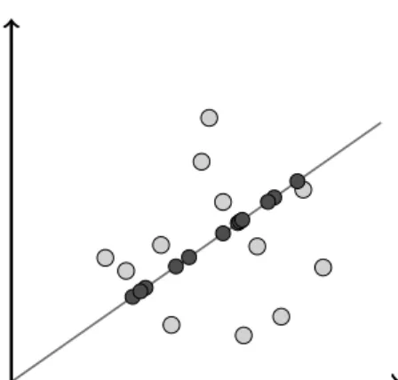
Figure 1: Vizualization of a point set that is projected down to a 1-dimensional subspace. Notice that both subspace here and in all other pictures are of the same dimension to keep the picture 2-dimensional, but the query subspace should have smaller dimension. where the first equality follows since U has or-thonormal columns, the second inequality since for M = VTX we have kDMk2 2 − kD(m)Mk22 = Pn i=1 Pn j=1sim2ij − P m i=1 Pn j=1sim2ij = Pn i=m+1 Pn j=1sim2ij = k(D − D(m))Mk2, and
the inequality follows because the spectral norm is consistent with the Euclidean norm. It follows for our choice ofmthat
jsm+1≤ε·(m−j+ 1)sm+1≤ε· m+1 X i=j+1 si≤ε· n X i=j+1 si. 2 In the following we will show that one can use the first m rows of D(m)VT as a coreset for the
linear j-dimensional subspace 1-clustering problem. We exploit the observation that by the Pythagorean theorem it holds that kAYk2
2 +kAXk22 = kAk22.
Thus, kAYk2
2 can be decomposed as the
differ-ence between kAk2
2, the squared lengths of the
points in A, and kAXk2
2, the squared lengths of
the projection of A on L. Now, when using U D(m)VT instead of A, kU D(m)VTYk2
2 decomposes
into kU D(m)VTk2
2 − kU D(m)VTXk22 in the same
way. By noting that kAk2
2 is actually Pn i=1si and kU D(m)VTk2 2 is Pm
i=1si, it is clear that storing the
remaining terms of the sum is sufficient to account for the difference between these two norms. Approxi-matingkAYk2
2bykU D(m)VTYk22thus reduces to
ap-proximatekAXk2
2bykU D(m)VTXk22. We show that
the difference between these two is only anε-fraction of kAYk2
2, and explain after the corollary why this
Figure 2: The distances of a point and its projection to a query subspace.
Lemma 6.2. (Coreset for Linear Subspace
1-Clustering) Let A ∈ Rn×n be an n×n matrix with
singular value decomposition A = U DVT, Y be
an n×(n−j) matrix with orthonormal columns, 0≤ε≤1, andm∈Nwithn−1≥m≥j+⌈j/ε⌉−1. Then 0≤ kU D(m)VTYk22+ n X i=m+1 si− kAYk22≤ε· kAYk22. Proof. We havekAYk2 2≤ kU D(m)VTYk22+kU(D− D(m))VTYk2 2≤ kU D(m)VTYk22+ Pn i=m+1si, which proves that kU D(m)VTYk2 2+P n i=m+1si− kAYk22 is
non-negative. We now follow the outline sketched above. By the Pythagorean Theorem, kAYk2
2 =
kAk2
2− kAXk22, where X has orthonormal columns
and spans the space orthogonal to the space spanned by Y. Using, kAk2 2 = Pn i=1si and, kU D(m)VTk22 = Pm i=1si, we obtain kU D(m)VTYk22+ n X i=m+1 si− kAYk22 = kU D(m)VTk2 2− kU D(m)VTXk22 + n X i=m+1 si− kAk22+kAXk22 = kAXk22− kU D(m)VTXk22 ≤ ε· n X i=j+1 si≤ε· kAYk22
where the first inequality follows from Lemma 6.1. 2 Now we observe that by orthonormality of the columns ofUwe havekU Mk2
2=kMk22for any matrix
M, which implies that kU DVTXk2
2 = kDVTXk22.
Thus, we can replace the matrix U D(m)VT in the
above corollary by D(m)VT. This is interesting,
because all rows except the first m rows of this new matrix have only 0 entries and so they don’t contribute tokD(m)VTXk2
2. Therefore, we will define
our coreset matrixS to be matrix consisting of the firstm=O(j/ε) rows ofD(m)VT. The rows of this
matrix will be the coreset points.
In the following, we summarize our results and state them fornpoints ind-dimensional space.
Corollary 6.1. Let Abe an n×nmatrix whose n rows represent n points inn-dimensional space. Let A=U DVT be the SVD ofAand letD(m)be a matrix
that contains the first m = O(j/ε) diagonal entries of D and is 0 otherwise. Then the rows of D(m)VT
form a coreset for the linear j-subspace 1-clustering problem.
If one is familiar with the coreset literature it may seem a bit strange that the resulting point set is unweighted, i.e. we replace n unweighted points bym unweighted points. However, for this problem the weighting can be implicitly done by scaling. Alternatively, we could also define our coreset to be the set of the firstmrows ofVT where theith row is
weighted bysi.
7 Dimensionality Reduction for Projective Clustering Problems
In order to deal withk subspaces we will use a form of dimensionality reduction. To define this reduction, letLbe a linear j-dimensional subspace represented by ann×j matrixX with orthonormal columns and withY being ann×(n−j) matrix with orthonormal columns that spansL⊥. Notice that for any matrix M we can write the projection of the points in the rows ofM toLasM XXT, and that these projected
points are still n-dimensional, but lie within the j -dimensional subspace L. Our first step will be to show that if we project both U DVT and A′ := U D(m)VT on X by computing U DVTXXT and
U D(m)VTXXT, then the sum of squared distances
of the corresponding rows of the projection is small compared to the cost of the projection. In other words, after the projection the points of A will be relatively close to their counterparts of A′. Notice the difference to the similar looking Lemma 6.1: In Lemma 6.1, we showed that if we project A toLand sum up the squaredlengths of the projections, then this sum is similar to the sum of the lengths of the projections ofA′. In the following corollary, we look at the distances between a projection of a point from A and the projection of the corresponding point in A′, then we square these distances and show that the
sum of them is small.
Corollary 7.1. Let A∈Rn×n and letA=U DVT
be its singular value decomposition. Let D(m) be a
matrix whose firstmdiagonal entries are the same as that of Dand let it be0, otherwise. LetX ∈Rn×j be
a matrix with orthonormal columns and let n−1 ≥ m ≥ j+⌈j/ε⌉ −1 and let Y ∈ Rn×(n−j) a matrix
with orthonormal columns that spans the orthogonal complement of the column space of X. Then
kU DVTXXT−U D(m)VTXXTk22≤ε· kAYk22 Proof. We havekU DVTXXT−U D(m)VTXXTk2 2= kDVTX − D(m)VTXk2 2 = kDVTXk22 − kD(m)VTXk2 2 = kU DVTXk22− kU D(m)VTXk22 ≤ εPn
i=j+1si ≤ εPni=1si ≤εkAYk22, where the third
last inequality follows from Lemma 6.1. 2 Now assume we want to use A′ = U D(m)VT
to estimate the cost of an j-dimensional affine sub-space k-clustering problem. Let L1, . . . , Lk be a set
of affine subspaces and let L be a j∗-dimensional subspace containing C = L1 ∪ · · · ∪ Lk, j∗ ≥
k(j+ 1). Then by the Pythagorean theorem we can write dist2(A, C) = dist2(A, L) + dist2(AXXT, C),
where X is a matrix with orthonormal columns whose span is L. We claim that dist2(A′, C) +
Pn
i=m+1si is a good approximation for dist2(A, C).
We also know that dist2(A′, C) = dist2(A′, L) + dist2(A′XXT, C). Furthermore, by Corollary
6.2, |dist2(A′, L) + Pn
i=m+1si − dist 2
(A, L)| ≤ εdist2(A, L) ≤ εdist2(A, C). Thus, if we can prove that |dist2(AXXT, C) − dist2(A′XXT)|2
2 ≤
ε · dist(A, C) we have shown that |dist(A, C) − (dist(A′, C) +Pn
i=m+1si)| ≤2εdist(A, C), which will
prove our dimensionality reduction result.
In order to do so, we can use the following ‘weak triangle inequality’, which is well known in the coreset literature, and can be generalized for other norms and distance functions (say, m-estimators).
Lemma 7.1. For any 1 > ε > 0, a compact set C⊆Rn, andp, q∈Rn, |dist2(p, C)−dist2(q, C)| ≤ 12kp−qk 2 ε + ε 2dist 2(p, C). 8 Proof of Lemma 7.1
Proof. Using the triangle inequality, |dist2(p, B)−dist2(q, B)|
=|dist(p, B)−dist(q, B)| ·(dist(p, B) + dist(q, B)) ≤ kp−qk ·(2dist(p, B) +kp−qk)
≤ kp−qk2+ 2dist(p, B)kp−qk. (8.4)
Either dist(p, B)≤ kp−qk/εorkp−qk< εdist(p, B). Hence, dist(p, B)kp−qk ≤ kp−qk 2 ε +εdist 2 (p, B). Combining the last inequality with (8.4) yields
|dist2(p, B)−dist2(q, B)| ≤ kp−qk2+2kp−qk 2 ε + 2εdist 2 (p, B) ≤ 3kp−qk 2 ε + 2εdist 2(p, B).
Finally, the lemma follows by replacingεwithε/4.2 We can combine the above lemma with Corollary 7.1 by replacing ε in the corollary with ε2/30 and
summing the error of approximating an input point p by its projection q. If C is contained in a j∗ -dimensional subspace, the error will be sufficiently small for m ≥ j∗+⌈30j∗/ε2⌉ −1. This is done in
the proof of the theorem below.
Theorem 8.1. Let A ∈ Rn×n be a matrix with
singular value decomposition A = U DVT and let
ε > 0. Let j ≥ 1 be an integer, j∗ = j + 1 and m = j∗ + ⌈30j∗/ε2⌉ − 1 such that m ≤ n− 1.
Furthermore, let A′ = U D(m)VT, where D(m) is a
diagonal matrix whose diagonal is the firstmdiagonal entries of D followed byn−mzeros.
Then for any compact set C, which is contained in aj-dimensional subspace, we have
dist2(A, C)− dist2(A′, C) + n X i=m+1 si ! ≤ε·dist2(A, C).
Proof. Suppose that X ∈Rn×(j+1) has orthonormal
columns that spanC. LetY ∈Rn×(n−(j+1)) denote a
matrix whose orthonormal columns are also orthogo-nal to the columns ofX. SincekAYk2is the sum of
squared distances to the column space ofX, we have (8.5) kAYk2≤dist2(A, C).
Fix an integer i, 1 ≤ i ≤ n, and let pi denote
theith row of the matrix AXXT. That is, p i is the
projection of a row ofAonX. Letp′
i denote theith
row ofA′XXT. Using Corollary 7.1, while replacing
εwithε′ =ε2/30 n X i=1 kpi−p′ik2 (8.6) =kU DV XXT−U D(m)V XXTk2 ≤ε 2 30· kAYk 2.
Notice that if ui is the ith row of U, then the
ith row of A can be written as Ai∗ = uiDVT,
and thus for its projection p to X it holds p = uiDVTXXT. Similarly,p′=uiD(m)VTXXT. Thus,
the sum of the squared distances between all p and their corresponding p′ is just ||U DVTXXT −
U D(m)VTXXT||2
2, which is bounded byε′||AY||2 by
Corollary 7.1 and since we setm=j∗+⌈30j∗/ε2⌉ −1
in the precondition of this Theorem. Together, we get
dist2(A, C)−dist2(A′, C)− n X i=j+1 si = kAYk2− kA′Yk2 (8.7) − n X i=j+1 si+ X p∈P (dist2(p, C)−dist2(p′, C)) ≤ε′kAYk2 (8.8) + n X i=1 12 kpi−p′ik2 ε + ε 2 ·dist 2(p i, C) ≤ ε′+12ε ′ ε + ε 2 dist2(A, C) (8.9) ≤εdist2(A, C),
where (8.7) follows from the Pythagorean Theo-rem, (8.8) follows from Lemma 7.1 and Corollary 6.2, and (8.9) follows from (8.5) and (8.6). 2 9 Small Coresets for Projective Clustering In this section we use the result of the previous section to prove that there is a strong coreset of size independent of the dimension of the space. In the last section, we showed that the projection A′ of A is a coreset forA. A′ still hasnpoints, which are n -dimensional but lie in anm-dimensional subspace. To reduce the number of points, we want to apply known coreset constructions toA′within the low dimensional subspace. However, this would mean that our coreset only holds for centers that are also from the low dimensional subspace, but of course we want that the centers can be chosen from the full dimensional space. We get around this problem by applying the coreset constructions to a slightly larger space than the subspace that A′ lives in. The following lemma provides us the necessary tool to complete the argumentation.
Lemma 9.1. Let L1 be a d1-dimensional subspace of Rnand letLbe a(d1+d2)-dimensional subspace ofRn
that containsL1. LetL2be ad2-dimensional subspace
of Rn. Then there is an orthonormal matrix U such
that U x = x for any x ∈ L1 and U x ∈ L for any
x∈L2.
Proof. Let B1 be an n×n matrix whose columns
are an orthonormal basis of Rn such that the first
d1 columns span L1 and the first d1 +d2 columns
span L2. Let B2 an n×n matrix whose columns
are an orthonormal basis ofRn such that the firstd1
columns are identical with B1 and the first d1+d2
columns span L2. Define U = B1B2T. It is easy to
verify thatU satisfies the conditions of the lemma. 2
Let L be any m+j∗-dimensional subspace that contains the m-dimensional subspace in which the points inA′ lie, let C be an arbitrary compact set, which can, for example, be a set of centers (points, lines, subspaces, rings, etc.) and let L2 be a j∗
-dimensional subspace that containsC. If we now set d1 := m and d2 := j∗ and let L1 be the subspace
spanned by the rows of A′, then Lemma 9.1 implies that every given compact set (and so any set of centers) can be rotated intoL. We could now proceed by computing a coreset in a m + j∗-dimensional subspace and then rotate every set of centers to this subspace. However, the last step is not necessary because of the following.
The mapping defined by any orthonormal matrix Uis an isometry, and thus applying it does not change Euclidean distances. So, Lemma 9.1 implies that the sum of squared distances of C to the rows of A′ is the same as the sum of squared distances of U(C) :={U x : x∈C} to A′. Now assume that we have a coreset for the subspaceL. U(C) is still a union ofk subspaces, and it is in L. This implies that the sum of squared distances to U(C) is approximated by the coreset. But this is identical to the sum of squared distances to C and so this is approximated by the coreset as well.
Thus, in order to construct a coreset for a set of n points in Rn we proceed as follows. In a first
step we use the dimensionality reduction to reduce the input point set to a set ofnpoints that lie in an m-dimensional subspace. Then we construct a coreset for a (d+j∗)-dimensional subspace that contains the low-dimensional point set. By the discussion above, this will be a coreset.
Finally, combining this with known results [21, 19, 36] we gain the following corolarry.
Corollary 9.1. LetP be a set of points inRd, and
k, j ≥ 0 be a pair of integers. There is a set Q in
Rd, a weight functionw:Q→[0,∞) and a constant
c >0 such that the following holds.
j-subspaces of Rd we have (1−ε)X p∈P dist2(p, B)≤X p∈Q w(p)dist2(p, B) +c ≤(1 +ε)X p∈P dist2(p, B), and 1. |Q|=O(j/ε)if k= 1 2. |Q|=O(k2/ε4)if j= 0 3. |Q|= poly(2klogn,1/ε)if j= 1,
4. |Q| = poly(2kj,1/ε) if j, k > 1, under the
assumption that the coordinates of the points in P are integers between 1 andnO(1).
In particular the size of Qis independent ofd.
10 Fast, streaming, and parallel
implementations
One major advantage of coresets is that they can be constructed in parallel as well as in a streaming setting.
That are can be constructed (‘embarrassingly’) in parallel is due to the fact that the union of coresets is again a coreset. More precisely, if a data set is split into ℓ subsets, and we compute a (1 + ε′ )-coreset of size s for every subset, then the union of the ℓ coresets is a (1 +ε′)-coreset of the whole data set and has size ℓ·s. This is especially helpful if the data is already given in a distributed fashion on ℓ different machines. Then, every machine will simply compute a coreset. The small coresets can then be sent to a master device which approximately solves the optimization problem. Our coreset results for subspace approximation for one j-dimensional subspace, for k-means and for general projective clustering thus directly lead to distributed algorithms for solving these problems approximately.
If we want to compute a coreset with size indepen-dent ofℓon the master device or in a parallel setting where the data was split and the coresets are later collected, then we can compute a (1 +ε′)-coreset of this merged coreset, gaining a (1 +ε′)2-coreset. For
ε′ := ε/3, this results in a (1 +ε)-coreset because (1 +ε/3)2<1 +ε.
In the streaming setting, data points arrive one by one, in which it is impossible to remember the entire data set due to memory constraints. We state a failry general variant of the technique ‘Merge & Reduce’ [29] allowing us to use coresets in a stream while also being able to compute in parallel. For this, we define the notion of coreset schemes.
The following definition is a generalization of Definition 2, where the ground setX=Rd×[0,∞)×
[0,∞) is the set of points in Rd, each assigned with
multiplicative and additive weight,Q is all k-tuples ofj-dimensional query subspaces inRdfor some fixed
j, k ≥ 1. For a given pair j, k ≥ 1 of integers, a coreset scheme for the (j, k)-projective clustering problem Alg(P, ε) is an algorithm whose input is a setP ⊆X of weighted points and an error parameter ε. It outputs a setC (called coreset) such that for every query subspaceL∈Q, its cost
f(P, q) := X (p,w,w′ )∈P w·dist2(p, L) + X (p,w,w′ )∈P w′ approximated, up to a factor of (1±ε), byf(C, q). In Definition 2, we denote c = P (p,w,w′)∈Cw′ and assumed thatP has no weights. However, in the merged-and-reduce approach that is described in this section, we apply the algorithm Alg recursively on its output coresets, and thus must assume that the input is also weighted. Since the distribution of the additive weights across the points has no effect onf, we can assume that only one arbitrary point inP has a positive additive weight.
Definition 3. (Coreset Scheme) LetXandQbe two sets. Let f : 2X ×Q → [0,∞) be a function
that maps every subset ofX and q∈Q to a positive real. An ε-coreset scheme Alg(·,·) for (X, Q) is an algorithm that gets as input a set P ⊆ X and a parameter ε ∈ (0,1/10). It then returns a subset C := A(P, ε) of X such that for every q ∈ Q we have
(1−ε)f(C, q)≤f(P, q)≤(1 +ε)f(C, q) The following theorem is a generalized and im-proved version of the coreset for streaming k-means from [29, Theorem 7.2]. The improvement is due to the use of (ε/logn)-coresets rather than (ε/log2n )-coresets, which are usually constructed in less time and space. Similar generalizations have been used in other papers. The proof uses certain composition properties that coresets satisfy.
Theorem 10.1. Let X be a set representing a (pos-sibly unbounded) stream of items, let Q be a set ε∈ (0,1/10)and let Alg(·,·)be an ε-coreset scheme for(X, Q). Suppose that for every input setP ⊆X of |P| ≤n′ items, and every ε∈(0,1/10)we can com-pute a coresetAlg(P, ε)of size at mosta(ε, n′)using at mostt(ε, n′)time ands(ε, n′)space, and that there is an integerm(ε)such that a(ε,2m(ε))≤m(ε).
Then, we can dynamically maintain an ε-coreset C for the n items seen so far at any point in the stream, where
Figure 3: Tree construction for generating coresets in parallel or from a data stream. Black arrows indi-cate ‘merge-and-reduce’ operations. The (intermedi-ate) coresetsC1, . . . , C7 are enumerated in the order
in which they would be generated in the streaming case. In the parallel case,C1, C2, C4andC5would be
constructed in parallel, followed by parallel construc-tion ofC3andC6, finally resulting inC7. The figure
is taken from [33].
(i) it holds|C| ≤a(ε′/9, m(ε′)·O(logn))for an ε′ =O(ε/logn).
(ii) The construction of C takes at most s(ε′,2m(ε′)) +s(ε/9, m(ε′)·O(logn)) space with additional m(ε′)·O(logn)items. (iii) Update time of C per point insertion to the
stream is
t(ε′,2m(ε′))·O(logn) +t(ε/9, O(m(ε′) logn)) (iv) The amortized update time can be divided byM
usingM ≥1 processors in parallel.
Proof. We first show how to construct an ε-coreset only for the firstnitemsp1,· · ·, pn in the stream, for
a givenn≥2, using space and update time as in(i) and(ii).
Put ε′ = ε/(6⌈logn⌉) and denote m′ = m(ε′). Theε′-coreset of the first 2m′−1 items in the stream is simply their union. After the insertion of p2m′ we replace the first 2m′ items by theirε′-coresetC
1.
The coreset forp1,· · · , p2m′+i is the union ofC1 and
p2m′+1,· · ·, p2m′+i for every i = 1,· · ·,2m. When
p4m′ is inserted, we replacep2m′+1,· · ·, p4m′ by their
ε′-coresetC
2. Using the assumption of the theorem,
we have|C1|+|C2| ≤2m′. We can thus compute an
ε′-coreset of size at mostm′ for the union of coresets C1∪C2, and deleteC1and C2 from memory.
We continue to construct a binary tree of coresets as in Fig. 3. That is, every leaf and node contains at
mostm′items. Whenever we have two coresets in the same level, we replace them by a coreset in a higher level. The height of the tree is bounded from above by⌈logn⌉. Hence, in every given moment during the streaming ofn items, there are at mostO(logn) ε′ -coresets in memory, each of size at mostm′. For any n, we can obtain a coreset for the first n points at the moment after they the nth point was added by computing an (ε/3)-coresetC for the union of these at mostO(logn) coresets in the memory.
The approximation error of a coreset in the tree with respect to its leaves (the original items) is increased by a multiplicative factor of (1+ε′) in every tree level. Hence, the overall multiplicative error of the union of coresets in memory is (1+ε′)⌈logn⌉. Using the definition ofε′, we obtain
(1 +ε′)⌈logn⌉= (1 + ε 6⌈logn⌉)
⌈logn⌉≤eε
6 <1 +ε/3.
Since (1 +ε/3)2 ≤ 1 +ε by the assumption ε ∈
(0,1/10), we have thatCis anε-coreset for the union of all then items seen so far. We now prove claims (i)-(iv) for fixedn.
(i) C is an ε/3 coreset for O(logn) sets of size m′, and thus|C|=a(ε/3, m′·O(logn))
(i) In every item insertion, there are O(logn) coresets in memory, each of size at most m′, and additional O(m) items at the leaves. Since we use additional space ofs(ε′,2m′) for constructing a coreset in the tree, ands(ε/3, m′·O(logn)) space for constructingC, the overall space for the construction is bounded by
s(ε′,2m′) +s(ε/3, m′·O(logn)) with additionalm′·O(logn) items.
(ii) When a new item is inserted, we need to apply the coreset construction at mostO(logn) times, once for each level. Together with the computation time ofC, the overall time is
t(ε′,2m′)·O(logn) +t(ε/3, O(m′logn)) per point insertion.
(iii) follows since the coresets can be computed in parallel for each level. More precisely, then/(2im′) coresets in theith level can be computed in parallel by dividing them into min
M, n/(2im′) machines. The main problem with the above construction is that it assumes that n is known in advance. To remove this assumption, we compute the above coresets tree independently for batches (sets) with exponentially increasing size: a tree for the first batch ofn1= 2m′ items in the stream (which consists of a
n2= 4m′items, and in general a tree forith batch of
the followingni= 2im items in the stream fori≥1.
For every i ≥ 1, let εi = ε/(3clogni) and
compute an εi-coreset in each node of the ith tree,
rather than ε′-coreset. After all the n
i items of the
ith batch were read, its tree consists of a single (root) (ε/3)-coresetCi of its ni leaves, where|Ci|=m(εi).
After insertion of the nth item to the stream to the current jth batch, we havej=O(logn). We output an (ε/3)-coresetC for the union of previous coresets C1∪C2∪. . .∪Cj−1with theO(logn) (εj)-coresets in
the current (last) tree. Hence,Cis anε-coreset for the nitems. Its size is union of theO(logn) (ε/(3clogn ))-coresets in its tree. Hence, Cj is an (ε/3)-coreset for
the items that were read in the current batch, and thus C1 ∪C2 ∪ · · · ∪Cj is an (ε/3)-coreset for all
the nitems. We then output an (ε/3)-coresetC for C1∪C2∪ · · · ∪Cj, which is an ε-coreset for the n
items. The space and time bounds are dominated by the last batch of size nj ≤n, so the time and space
have the same bounds as above for a fixed set of size n.
For parallel construction of an unbounded stream, we simply send theith point in the stream to machine number (i modM) for every i ≥ 1. Each machine computes a coreset to its given sub-stream, as explained above for a single machine. The coreset in every given moment is the union of current core-sets in all theM machines. It may then be written in parallel to a shared memory on one of the machines. 2 11 Small Coresets for Other Dissimilarity
Measures
In this section, we describe an alternative way to prove the existence of coresets independent of the number of input points and the dimension. It has an exponential dependency onε−1and thus leads to
larger coresets for k-means. However, we show that the construction also works for a restricted class of µ-similar Bregman divergences, indicating that it is applicable to a wider class of distance functions. Setting.
We are interested in formulating our strategy for more general distance measures than only l2. Thus,
for the formulation of the needed conditions, we just assume any distance function d : Rd ×Rd → R≥0
which satisfiesd(0) = 0. As usually, we use the abbre-viations cost(U) = min
z∈V P x∈Ud(x, z), cost(U, C) = P x∈U min
c∈Cd(x, c) and opt(U, k) = C⊂minV,|C|=kcost(U, C)
for U, C ⊂Rd. We are interested in a coreset Z for
P for approximate computation of opt(P, C) given an
arbitrary setCofkcenters.
Clustering Features. A classical coreset is be a weighted set of points, for which the clustering cost is computed in a weighted fashion. In the sections above, we already saw that it can be beneficial to deviate from this definition. Here, we will construct a coreset consisting of so called clustering features. These are motivated by the well-known formula
X p∈P d(p, z) (11.10) =|P′|d(z, µ(P)) +X p∈P d(p, µ(P))
that holds for squared Euclidean distances as well as for Bregman divergences, if µ(P′) denotes the centroid of P′. With help of 11.10, the sum of the distances of points in a set P′ to a center c can be calculated exactly when only given the clustering features|P|,P
p∈Ppand
P
p∈Pd(p,0).
When given a CF and a set of centers, then the optimal choice to cluster the points represented by the clustering feature without splitting them is to assign them to the center closest to the centroid of the CF, which follows from 11.10. Thus, when clustering a set of CFs Z with a set of centers C we define the clustering cost costCF(Z, C) as the cost for clustering
every CF with the center closest to its centroid. We are interested in the following coreset type.
Definition 4. Let P be a point set in Rd. Let
d:Rd×Rd→Rbe a distance measure that satisfies
11.10. A CF-coreset is a set of clustering features consisting of|P|,P
p∈Ppand
P
p∈Pd(p,0), such that
|cost(P, C)−costCF(Z, C)| ≤ε·cost(P, C)
holds for every setC of k centers.
In the following, we abbreviate CF-coreset by coreset. Notice that the error of the coreset compared toP is only induced by points which where summa-rized in one clustering feature but would optimally be clustered with different centers fromC.
Construction and Sufficient Conditions. Although we are mainly interested in CF-coresets, our algorithm will also work for other dis-tance functions, also if they do not satisfy 11.10, if the distance function satisfies the following two con-ditions. This is independent of the actual definition of the coreset used, as long as the coreset approximates the cost as in Definition 4. We thus formulate the conditions and the algorithm for any distance func-tion with any coreset nofunc-tion, and costc denotes the
cost function used for clustering with the unknown coreset type.