Evolution of Collaboration in Open Source Software Ecosystems

(1)

Evolution of Collaboration in Open

Source Software Ecosystems

Jos van der Maas

[email protected]

Department of Information and Computing Sciences Master in Business Informatics

January 2016

MSc thesis under supervision of:

First supervisor: Dr. S. Jansen (Utrecht University) Second supervisor: Dr. F.J. Bex (Utrecht University)

(2)

Abstract

Although in the past decennium much research has been conducted in the field of software ecosystems, still little is known about how such ecosystems evolve. In existing literature, software ecosystems are often analyzed from a single point of time, without regard for their dynamic history.

We study an aspect of the evolution of open source software ecosystems: collaboration. In this thesis, we present a method to identify and analyze collaboration networks in software ecosystems, based on historical data from the online source code hosting service GitHub. We apply this method to analyze the evolution of collaboration within the well-established open source ecosystem around the Ruby programming language. Our method can be used to identify and visualize collaboration networks around a given actor or software component over the course of time. This is done using statistical analysis techniques, without requiring subjective input. Our study analyzes over 200 collaboration networks to identify typical life cycle shapes and gives insight in the evolution an open source software ecosystem. Awareness of such collaboration networks and how they evolve is beneficial for actors in software ecosystems and for external stakeholders.

(3)

Acknowledgements

This Master’s thesis is the result of a research project that took several months. Looking back at this period, I am thankful to several people.

First of all, I would like to thank my first supervisor Slinger Jansen for his time, his quick and constructive feedback, and his insightful recommendations. Slinger, thanks for your supervision and the directions you gave by email, Skype, and face-to-face. I could not have wished a better supervisor.

In the second place, I would like to thank my other supervisor Floris Bex for his feedback and for reviewing this thesis document. I would also like to thank the other staff members of the Center for Organization & Information for the MBI study program, which I really appreciated.

I would like to thank my colleagues for allowing me to work part-time while doing my thesis research, my parents for their interest in my study progress, my wife for her support and our five months old son for sleeping well at night and allowing me to rest enough to finish this thesis project.

(4)

Introduction

“If you think the industrial revolution was transformational, the App Store is way bigger”.

This statement appeared in a video1 _{aired at Apple’s World Wide Developers Conference in June 2015.}

Although at first sounding like exaggerated marketing talk, the remark originates from the director of the McKinsey Global Institute, a research group concentrating on major economic trends around the world. Many other scientific sources acknowledge the impact of the introduction of app stores, which are market-places for applications that can be instantly downloaded and installed on a customer’s device. Jansen & Bloemendal (2013) call it “one of the most powerful changes that the software business currently is experi-encing” and Miluzzo, Lane, Lu, & Campbell (2010) speak about “a new era”.

In a broader sense, we observe that, especially since the introduction of the Internet, software is often built around a certain technological platform or market it interacts with (Bosch, 2009; Molder, Van Lier, & Jansen, 2011). Examples such technological platforms or markets are: app stores for mobile applications (such those facilitated by Apple, Google and Microsoft), the Ruby programming language with its network of ‘gems’ that often depend on other Ruby gems2_{, and online CMSes like Wordpress}3_{, Joomla}4_{, and Drupal}5_{, each}

with its own community of users and numerous available plugins.

In general, we observe that “networks of interrelated organizations form themselves around products, plat-forms, technologies or software organizations” (van Angeren, 2013). Such networks are referred to assoftware ecosystems (Messerschmitt & Szyperski, 2003). Jansen, Finkelstein, & Brinkkemper (2009) define a software ecosystem as

“a set of actors functioning as a unit and interacting with a shared market for software and services, together with the relationships among them. These relationships are frequently un-derpinned by a common technological platform or market and operate through the exchange of information, resources and artifacts”.

1_{https://www.youtube.com/watch?v=fSiDIaab2nY&t=72} 2_{See https://rubygems.org/}

3_{https://wordpress.org/} 4_{http://www.joomla.org/} 5_{https://www.drupal.org/}

(7)

Other definitions differ from the above one by putting more emphasis on relationships between software components. The choice of definition determines how software ecosystems are analyzed and visualized. Several authors have suggested methods to visualize software ecosystems, mostly by depicting ecosystems as networks. However, there is no widely accepted visualization method yet (Boucharas, Jansen, & Brinkkem-per, 2009; Goeminne & Mens, 2010; Campbell & Ahmed, 2010; Pérez, Deshayes, Goeminne, & Mens, 2012). Open source software ecosystems are especially suitable for research. Version control systems such as Git6 and Subversion7 _{keep exact records of changes in program code, in addition to information about authors}

and software dependencies. This data is often publicly available, making it possible to analyze open source ecosystems based on objective data. Collaboration is a key aspect of open source software, which can be measured by mining software repositories, from which collaboration networks can be identified. These networks can then be analyzed using scientific techniques from graph theory.

In recent years, researchers have made the connection between software ecosystems and (product) life cycles (dos Santos & Werner, 2011; Kim, Lee, & Altmann, 2014). Such research aims to capture life cycles of software ecosystems, describing various typical stages, such as emergence, maturity and downfall.

To study life cycles of collaboration networks in software ecosystems, longitudinal research is required. For many open source ecosystems however, a detailed history of changes is already publicly available, including timestamps, author information, and information about the content of the changes. This opens possibilities to study life cycles of collaboration networks based on historical data, without having to follow the actors in the networks for a longer period of time.

6_{https://git-scm.com/}

(8)

1.1 Problem Statement

Still much is unclear about the evolution of software ecosystems. This problem can be broken down into three or four sub-problems, as described below.

Static view

In existing scientific literature, the state of a software ecosystem is often observed from one specific point in time, instead of being regarded as a continuous evolutionary process. For example, Kabbedijk & Jansen (2011) give a detailed network visualization of the Ruby ecosystem. However, the visualization shows the status of the ecosystem for one point in time, namely the time when the research was carried out. The authors acknowledge that “due to the lack of longitudinal data it is impossible to speculate about the dynamics of the Ruby SECO [software ecosystem]”.

A similar situation is found in the study of Blincoe, Harrison, & Damian (2015). This publication gives a visualization of multiple software ecosystems for which the code is hosted on GitHub, but again only for a single point in time.

In this respect, van Angeren (2013) remarks that

“a longitudinal case study of proprietary platform ecosystems could benefit a wealth to the un-derstanding of the fast-paced dynamics characteristic for the software industry”.

Similarly, Kim, Altmann, & Lee (2013) remark that

“prior research concentrates only on the static properties of network structure and the position of nodes in the network, but misses the dynamics in the evolution context”.

Insight in this “dynamics in the evolution context” is important for our understanding of software ecosystems.

Validity of life cycle models

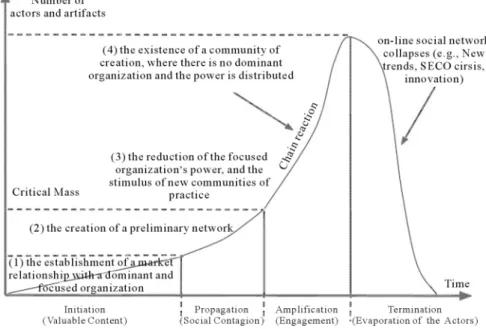
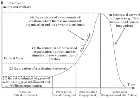
While there exists some scientific theory on software ecosystem evolution and especially on ecosystem life cycles, this theory needs to be validated. For example, dos Santos, Esteves, Freitas, & de Souza (2014) suggest that a software ecosystem life cycle goes through the consecutive phases of Initiation, Propagation, Amplification, and Termination, following a curve as shown in Figure 1.1.1. Kim, Lee, & Altmann (2014) mention three phases: Ascent/Emergence, Maturity/Prosperity, and Decline.

The theory of ecosystem size following a path along consecutive stages originates from product life cycle theory, such as the work of Polli & Cook (1969) and Tellis & Crawford (1981). However, it is unclear whether this theory can be readily applied to the dynamic nature of software ecosystems. Such an assumption must be tested in practice.

(9)

Figure 1.1.1: Software ecosystem maturity model proposed by dos Santos et al. (2014).

Small samples

Another problem is that existing analysis of software ecosystems is often based on relatively small samples, i.e. a small number of networks that is analyzed per publication. It would be interesting to analyze and compare a large number of networks to each other.

Many publications are limited to only one well-established software ecosystem, such as Eclipse (Dhungana, Groher, Schludermann, & Biffl, 2010), Ruby (Kabbedijk & Jansen, 2011), or Apache (Santana & Werner, 2013). Few studies try to compare data from multiple ecosystems to each other.

Domain-specific measurement of ecosystem relationships

It is debatable how relationships in software ecosystems should be identified. Going back to the definition of Jansen et al. (2009), we see that a software ecosystem is “a set of actors (...), together with the relationships among them”. Other definitions of software ecosystems are similar in the sense that they tell us that there are some kind of ‘relationships’ between actors or software components. However, in what way these relationships can be tracked or measured is subject to wide interpretation.

In existing literature, data for measurement of relationships in software ecosystems is often collected from a domain-specific source, such as the Gnome website8 _{for the Gnome ecosystem (Mens & Goeminne, 2011)}

and the RubyGems website9 _{for the Ruby ecosystem (Kabbedijk & Jansen, 2011). However, the way in}

which such data is collected differs and is often difficult to generalize for other ecosystems.

8_{https://www.gnome.org/} 9_{https://rubygems.org/}

(10)

Summary

In short, these issues can be captured in the following problem statement:

It is unclear how collaboration in open source software ecosystems evolves. Existing research fails to longitudinally analyze a substantial amount of collaboration data in a generalizable way.

We will narrow our research scope toopen sourcesoftware ecosystems, as reflected in this problem statement.

Approach outline

In order to address the stated problem, we propose to use historical data from GitHub10, which is the largest online open source code repository (Gousios, Vasilescu, Serebrenik, & Zaidman, 2014), as data source. This data contains precise information about changes in program code of thousands of open source projects. The data is publicly available and can be queried to reconstruct time-specific collaboration networks. These networks are then analyzed to study the evolution of collaboration in open source software ecosystems.

(11)

1.2 Research Questions

The main research question addressed in this thesis is:

How does collaboration in open source software ecosystems evolve? In order to answer this research question, we formulate the following sub research questions:

1. What are relationships in software ecosystems? The way in which relationships in software ecosystems are measured is of crucial importance for the further analysis of these ecosystems. In the past, researchers have chosen to base relationships on, amongst others, co-authorship (Kabbedijk & Jansen, 2011), API implementation (Kim, Lee, & Altmann, 2014), and the use of cross-references (Blincoe, Harrison, & Damian, 2015). Furthermore, the information sources for the determination of such relationships vary from mailing lists (Bird, Gourley, Devanbu, Gertz, & Swaminathan, 2006) to domain-specific websites (Hoving, Slot, & Jansen, 2013), surveys (Syed & Jansen, 2013), and com-pany websites (van Angeren, Alves, & Jansen, 2014). We study similarities and differences between these determination methods in our literature review and propose a definition of software ecosystem relationships.

2. How can collaboration in software ecosystems be measured and visualized, based on data from a public data source? We query historical data from a public data source (GitHub) to identify collaboration networks and measure their state. The state of a network can be measured using several properties. For example, van Angeren et al. (2014) use the properties Size, Density, Degree centrality, Centralization, Modularity, and Clustering. We calculate similar properties for collaboration networks on a day-to-day basis to analyze their life cycles.

3. Can various categories of collaboration networks be distinguished, based on their life cycles? An important question is to which extent (product) life cycle stages such as Initiation, Propagation, Amplification, and Termination are applicable to collaboration in open source ecosystems. Our hypothesis is that the life cycles of certain collaboration network fit these stages, whiles others have a completely different cycle. We aim to discover a concise number of categories of collaboration networks that resemble each other in terms of their life cycles. Using a sample set of randomly selected networks, we study such categories.

4. How are the collaboration networks in these categories characterized? Once we have es-tablished a number of life cycle categories, we study which characteristics or properties are typical for these categories. For example, are there certain deviations in the network structure of collaboration network that are a good indicator for the approximate life cycle course?

5. How does collaboration in an open source ecosystem evolve in practice? This question is addressed by a case study on the ecosystem around the Ruby programming language.

To provide an answer to the (sub) research questions, data from the GitHub Archive11 (a project that maintains a history of GitHub data) will be gathered in a database and a tool will be developed that can

(12)

identify collaboration networks, starting from a single project or author. The tool will then be used to compare and analyze a large number of networks using statistical analysis techniques.

1.3 Relevance

1.3.1 Scientific Relevance

Due to its recentness, the research domain of software ecosystems leaves opportunities for research unad-dressed (Barbosa & Alves, 2011; Manikas & Hansen, 2013). Although relatively much research has been conducted on open source ecosystems and modeling (Barbosa & Alves, 2011), the research field of software ecosystem evolution is still largely unexplored.

A large proportion of the literature on software ecosystems consists of case studies on single predefined ecosystems. Limited attempts have been made to conduct a thorough quantitative analysis, comparing a significant number of networks to each other.

Longitudinal studies on software ecosystems are rare. Our research will give insight in ecosystem evolution and life cycle categories. Theory about life cycle maturity stages will either be substantiated or disproved. The results of our research could be useful for prediction of evolution of ecosystems in their early stages. The tool that is developed as part of the research is useful for further in-depth research, e.g. about actor roles and their impact on the evolution of ecosystems.

1.3.2 Practical Relevance

Apart from its scientific relevance, our research has several benefits for practitioners.

Our study will facilitate the identification and exploration of open source ecosystems. As Blincoe et al. (2015) state in their research agenda: “A tool could be developed that automatically identifies technical dependencies across projects and provides a visualization of the ecosystem. Such a tool could increase awareness of coordination needs that extend outside project boundaries and help developers gain a better view of the ecosystem surrounding their project.” Awareness of the ecosystem around a software project can greatly benefit its developers.

For facilitators of ecosystems (such as the Eclipse Foundation12), insight in the development of ecosystems would be of great value to help stimulate the growth and increase the maturity and robustness of their ecosystem.

Furthermore, this research provides insight into the characteristics of different categories of collaboration networks. Once known which characteristics should be pursued and which should be avoided, strategical decisions can be made in the development of software projects.

(13)

1.4 Document Structure

After its introduction in Chapter 1, this thesis continues with an explanation of the research approach in Chapter 2. The next chapter contains the theoretical background for our research, answering our first research question.

Chapter 4 describes the development of the analysis tool and aims to answer the second research question. After this, Chapter 5 describes categories of collaboration networks and contains the results of the analysis of research question 3. Chapter 6 addresses the fourth research question, describing characteristics of software ecosystem categories.

The analysis part from Chapters 3 to 6 is followed by a case study of the Ruby ecosystem in Chapter 7, a summary and discussion of the research findings in Chapter 8, also containing suggestions for future research. The thesis ends with a conclusion in Chapter 9.

(14)

Chapter 2

Research Approach

Our research approach can be summarized as follows:

• Conduct a literature study on software ecosystems in general and software ecosystem relationships, characteristics, visualization, and analysis.

• Use GitHub and the GitHub Archive1_{as data source.}

• Define a method for measuring relationships and use this to identify collaboration networks for an arbitrary repository or developer as origin of the network.

• Develop a tool that can query the data to visualize the state of a collaboration network on a certain point in time.

• Let the tool follow the state of collaboration networks over time to obtain graphs depicting their life cycles.

• Define sample sets of open source collaboration networks on GitHub.

• Statistically analyze the life cycles of the networks in the sample set(s) to identify categories of collab-oration networks, based on their life cycles.

• Analyze the network properties of the categories to identify common network properties.

• Conduct a case study on the Ruby ecosystem to analyze how collaboration in ecosystems evolves in practice.

2.1 Literature Review

In this section, we describe the approach to conduct our literature review.

(15)

Method

We will use a scoped literature review, as described by Arksey & O’Malley (2005). In case of a scoped literature review (as opposed to a systematic literature review), a number of concrete consecutive steps can be followed to obtain a theoretical background for a research project. A scoped literature review aims to obtain information about a relatively broad topic, without seeking to address a specific study design or answer very specific research questions. As a result, there is less need to assess the quality of included studies. Scoped literature reviews can be also used to identify research gaps in existing literature (Arksey & O’Malley, 2005).

Systematic literature reviews for the research domain of software ecosystems have been conducted by Barbosa & Alves (2011) and Manikas & Hansen (2013). These studies revealed that the attention for software ecosystems is increasing, resulting in a large number of available publications on this topic.

Sources

To retrieve relevant sources for the literature review, our collection process consists of a number manual search queries for scientific contributions. Searches were performed on the scientific databases of ACM2_{, Emerald}3_,

IEEE4, Mendeley5, ScienceDirect6, Springer7, and Wiley8. The following keywords were combined into search strings:

(“software ecosystem” AND (“relationship” OR “network” OR “analysis” OR “evolution” OR “life cycle” OR “lifecycle” OR “visualization” OR “visualisation” OR “trend” OR “classification”)) OR “mining software repositories”

Where applicable, both the singular and plural forms of keywords were used. The following inclusion criteria were used to select sources for the literature review:

• All sources should be peer-reviewed scientific contributions. • All sources should be written in English.

To retrieve additional scientific sources, bibliographies of initially selected sources were reviewed. Relevant sources were considered based on their title, keywords, and abstract.

Relationships

In our literature review, we analyze how other scientific sources determine relationships. Based on the results from this literature review, we formulate our own definition of software ecosystem relationships.

2_{http://dl.acm.org/} 3_{http://www.emeraldinsight.com/} 4_{https://www.ieee.org/} 5_{https://www.mendeley.com/research-papers/} 6_{http://www.sciencedirect.com/} 7_{http://link.springer.com/} 8_{http://onlinelibrary.wiley.com}

(16)

2.2 Data Collection and Processing

Based on our definition of software ecosystem relationships, we define a method for identifying open source software ecosystems on GitHub. We limit our research to open source software ecosystems. An advantage of analyzing open source software is that the data is transparent, with much information being publicly available. Another advantage is that much of this information is objective, as opposed to e.g. survey data. A key characteristic of open source software is that it is generally developed by multiple developers at the same time. Therefore, we focus at collaboration relationships. We will analyze both relationships between software developers (actors) and software components.

Our goal is to analyze how software ecosystems develop over a period of time and to compare various stages in the life cycles of collaboration networks. For this, we need historical data, which we obtain by mining data of software repositories on GitHub.

Collaboration information on GitHub is stored in the form of commits, which can be pushed or requested to be pulled. Therefore, we analyze data from push events and (merged, i.e. successful) pull request events. To import and analyze the data, we build a web-based tool, which should at least have the following functionality:

• Importing data required for our analysis

• Establishing collaboration networks, based on co-authorship and starting from an arbitrary user or repository

• Visualizing these networks, over a period of time

• Visualizing network properties of these networks, based on literature from the literature review

2.3 Data Analysis

Based on our findings in the literature review, we obtain a sample set of collaboration networks and analyze how each of these networks evolves. We categorize the collaboration networks based on their life cycle shapes. We statistically test which life cycle shapes are most common. We also calculate the average life cycle for an open source ecosystem, based on our sample set. We do this for both repository-centered life cycles and user-centered life cycles.

We compare the most common life cycle categories to each other in terms of several network properties. We statistically test the differences between these categories.

After this, we analyze collaboration in a predefined open source ecosystem. We apply our analysis method to the Ruby ecosystem to see how an ecosystem evolves in practice over the course of several years.

2.4 Plan Validity

The validation of our research approach can be divided in four types of validity types.

Construct validity indicates that correct operational measures are used for the concepts that are studied. Internal validity is used for making sure that the casual relationships (where applicable) are properly linked.

(17)

Research is said to be externally valid if the findings are generalizable beyond the sample set. Reliability indicates that if someone else wants to continue our work, this should be possible. In other words, should someone else follow the same procedures as we did and conduct the same case studies, then the findings and conclusions should be the same.

2.4.1 Construct Validity

We propose to observe evolution of open source software ecosystems by measuring co-authorship based on push and (merged) pull request events. Instead of co-authorship, we could e.g. use email addresses or organization membership. Similarly, instead of pushes and pull requests, we could measure posted comments, opened issues, etc.

An advantage of looking at co-authorship is that this represent a natural connection in the real world, namely that of co-creation. Moreover, this relationships can be objectively measured. An advantage of using push and pull request evens is that the results do not depend on how much information a user specifies. E.g. email addresses can be omitted to prevent spam and organization membership might not (intentionally or unintentionally) be specified by a developer.

A limitation of our choice of measurement is that we do not measure the volume or impact of these events. E.g. the number of altered lines of code can vary widely per push and pull request event. However, on average the number of such events per user can be assumed to be a good indicator for the user’s activity. When many users make many pushes or pull requests, the ecosystem can be called alive and successful. When no more such events occur in a software ecosystem for several months (e.g. three months), the ecosystem can be assumed to have ended.

We will consider push and pull data per day. Instead of days, we could consider time intervals of hours, weeks, months, etc. However, using longer intervals (e.g. weeks) would result in relatively few data points, since we only have the years 2011-2015 as scope. Using shorter intervals (e.g. hours) would require significantly more computation power and could cause strong deviations caused by working hours, time zone differences, etc. As such, the choice of days as time intervals is appropriate and can be assume not to bias the results.

2.4.2 Internal Validity

Since the data is obtained from a public data source in retrospect, users do not know they are being studied for this research. Thus we can assume that they are not influenced by the measurement. We will use random selections to compose sample sets.

Life cycles of collaboration networks can be influenced by events outside our measurements, such as the temporary absence or death of a developer. However, such events can be regarded as part of the dynamics of software ecosystems.

2.4.3 External Validity

When it comes to external validity, our research has various limitations due to the choice of GitHub as data source:

(18)

• GitHub was launched in April 2008 and is therefore relatively new. However, it is currently the largest code host in the world, facilitating millions of developers collaborating across millions of repositories, according to Gousios, Vasilescu, Serebrenik, & Zaidman (2014).

• We have access to data of open source projects only. It is questionable whether or not this can be generalized to non-open source ecosystems. However, we limit our scope to open source software ecosystems.

• GitHub is not the only platform that facilitates open source software ecosystems. Not everything is hosted on GitHub. As Kalliamvakou, Gousios, Blincoe, Singer, German, & Damian (2014) write, “Many active projects do not conduct all their software development in GitHub”.

• GitHub only works with one version control system (Git, which was introduced in 2005).

• We obtain our data from the GitHub Archive project. This project has recorded data from February 12th_{, 2011 onwards.}

• Since we look at complete life cycles, we are limited to life cycles that fall within a the time period from early 2011 till mid 2015, a period of four years.

• It is possible that projects are hosted on GitHub that have existed prior to their submission to GitHub (e.g. projects that earlier used Subversion for version control). This will result in misleading activity numbers at the ‘start’ of such a software projects. However, since we only have data from 2011 and onwards and since GitHub already existed in 2008, these effects will likely be relatively low. Also, one large addition of code is only counted as a single event.

• Some features of GitHub, like organization membership, have not existed from the start of GitHub. But we will most likely not use these relatively new features for our research.

• In the research period, GitHub and the GitHub Archive Project had some downtime (i.e. were unac-cessible). However, from our database results it is clear that this downtime was relatively short and its effect insignificant for the results.

Despite these limitations, our approach makes it possible to study and compare a relatively large number of collaboration networks. Other studies have comparable limitations. Therefore we are confident that our research will shed new light on the evolution of open source software ecosystems.

2.4.4 Reliability

Part of our research will be the development of the tool to visualize and measure collaboration networks. This tool will be web-based, publicly accessible, and submitted as an open source project to GitHub. This tool can be used to verify our research and for further research.

(19)

Chapter 3

Literature Review

The concept ofsoftware ecosystemwas introduced by Messerschmitt & Szyperski (2003) and has since been the subject of extensive research. During the past decade, the number of scientific publications on Software Ecosystems (SECOs) has significantly increased (Barbosa & Alves, 2011; Manikas & Hansen, 2013). Our literature review will focus on the following subjects:

• Definitions of software ecosystems, in order to known precisely what we study. • Relationships in software ecosystems, to be able to analyze ecosystems as networks. • Network theory, to measure the state of the networks.

• Theory about evolution of software ecosystems, to help study our main research question. • Mining software repositories, to gather data for analyzing open source software ecosystems.

3.1 Definition of Software Ecosystems

Messerschmitt & Szyperski (2003) define a software ecosystem as

“a collection of software products that have some given degree of symbiotic relationships”.

While this to our best knowledge is the earliest formal definition of software ecosystems, the most cited definition is (according to Manikas & Hansen (2013)) that of Jansen, Finkelstein, & Brinkkemper (2009), who define a software ecosystem as

“a set of actors functioning as a unit and interacting with a shared market for software and services, together with the relationships among them. These relationships are frequently un-derpinned by a common technological platform or market and operate through the exchange of information, resources and artifacts”.

(20)

Other definitions that are commonly referred to are that of Bosch (2009):

“a set of software solutions that enable, support and automate the activities and transactions by the actors in the associated social or business ecosystem and the organizations that provide these solutions”

and the definition given by Lungu et al. (2010):

“a collection of software projects which are developed and evolve together in the same environ-ment”.

While these definitions vary, Manikas & Hansen (2013) remark that the definitions of software ecosystems to some extent contain the following three common elements:

1. A common software platform or environment;

2. A shared business or community; and

3. Connecting relationships.

The choice of definition has consequences for the perception of software ecosystems. In this thesis, we use the definition of Jansen et al. (2009), with the side note that relationships in software ecosystems can also be regarded at a software level, as further explained in the next section.

3.2 Relationships in Software Ecosystems

When analyzing software ecosystems, it is important what exactly one calls a relationship. In the definitions of software ecosystems we already observe differences. Some definitions speak of relationshipsbetween actors (e.g. the definition of Jansen et al.) and others of relationships between software components (e.g. the definition of Messerschmitt & Szyperski). These different views have consequences for the analysis and visualization of software ecosystems.

A number of examples from literature of what researchers choose as relationships is given below.

• Crowston & Howison (2005) base relationships between developers of open source projects on email addresses found in bug reports on public mailing lists.

• Bird, Gourley, Devanbu, Gertz, & Swaminathan (2006) base relationships between developers of open source software on public emails sent among them.

• Kabbedijk & Jansen (2011) base relationships in the Ruby ecosystem on co-authorship data from rubygems.org.

• Syed & Jansen (2013) base relationships between developers in the Ruby ecosystem on collaboration information from rubygems.org and a survey sent to a large number of developers.

• Hoving, Slot, & Jansen (2013) base relationships in the Python ecosystem on collaboration data from python.org.

(21)

• van Angeren, Alves, & Jansen (2014) base relationships between companies in the Google Apps software ecosystem on information found on company websites and on CrunchBase.com.

• Kim, Lee, & Altmann (2014) base relationships between providers of APIs and mashups that use those APIs on data from programmableweb.com.

• Gregorian (2014) bases relationships between GitHub developers on a complex formula that combines several forms of communication between the developers.

• Blincoe, Harrison, & Damian (2015) base relationships between GitHub repositories on cross-references between those repositories.

From these sources, we draw a number of conclusions:

1. Many different choices seem to be suitable to use as relationships. The concept of relationship is not strictly defined.

2. The essence of all relationships is the exchange of information. There must be some interaction or information exchange through the relationship.

3. Information exchange can exist between both actors (e.g. via emails) and software components (e.g. via an API).

4. In many cases, there is some common system or platform that facilitates the exchange of information (e.g. a mailing list or a code repository). Data from such a platform can be used to measure rela-tionships. This platform is often facilitated by what is called in literature a keystone (player). The information exchange can also be facilitated by a common technology, such as a software project or an API.

5. Relationships (in general) have the properties continuation and strength (Holmlund, 1997). The rela-tionships can be measured in terms of these properties.

6. The relationships are subject to continuous change because of their dynamic nature.

7. Relationships have potential because they provide access. They must be viewed in their context, in this case the ecosystem in which they are embedded.

From these conclusions, we formulate our own definition of software ecosystem relationships:

Definition. A relationship in a software ecosystem is a measurable dynamic form of informa-tion exchange between either two actors or two software components in the ecosystem. Such information exchange is often facilitated by a common technology or platform.

We can distinguish between explicitly measurable connections (e.g. commits to a software repository) and relationships that are open to human interpretation (e.g. surveys or information found on company websites). We observe that researchers often use an ecosystem-specific data source to measure relationships. This makes it less suitable to compare data from different software ecosystems to each other.

(22)

3.3 Network Perspective

Observing software ecosystems as networks consisting of nodes ands links opens possibilities for research and has two clear benefits. Firstly, networks provide a useful metaphor to communicate and interpret ecosystems and secondly, networks provide a basis for analytics through mathematical graph theory.

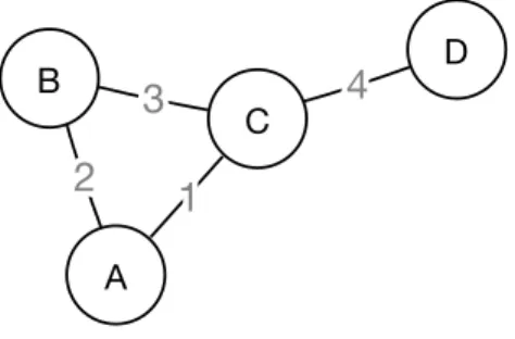
In literature, software ecosystems are often modeled as networks in the form of undirected graphs, implicating that the relations are symmetric (the relationship from A to B is the same as that from B to A). In our analysis, we use weighted undirected graphs, i.e. each relationship is given a numerical weight.

To analyze collaboration networks in software ecosystems, we use a number of well-established measures from graph theory. This is done on node level (focusing on the role of single nodes) as well as on network level (focusing on the state of a network as a whole).

A B C D

1

2

3

4

Figure 3.3.1: Example of an undirected weighted graph that could represent a Software Ecosystem consisting of nodes A, B, C, and D and the relationships among them.

3.3.1 Node Level Analysis

Degree

Thedegree of a node is defined as the number of edges connected to the node.

Formally defined, consider a graph withnnodes andadjacency functiona, meaning that for two given nodes piand pk in the network,

a(pi, pk) = (

1 if and only ifpi andpk are connected by an edge

0 otherwise. Then degree(pi) = n X i=1 a(pi, pk).

(23)

Weighted Degree

Theweighted degree of a node is the sum of the edge weights of its connecting edges. For example, node A in Figure 3.3.1 has a weighted degree of2 + 1 = 3. NodeDhas a lower degree than nodeA, but its weighted degree is higher.

Degree Centrality

Thecentrality of a node is a measure of how central a node in a network is compared to the other nodes. For example, in Figure 3.3.1 intuitively nodeC seems to be the most central node in the network. Freeman (1978) defines thedegree centrality of a nodepk in a graph withnnodes as follows.

relative degree centrality(pk) =

degree(pk)

n−1 .

Note that this is essentially the same as the degree of the node divided by the maximum degree it could possibly have (which isn−1, namely in case it is connected to all other nodes in the network). For example, the relative degree centrality of node C in Figure 3.3.1 is 4

5−1 = 1, since this node is connected to all the

other nodes in the network. Since the other nodes have lower degree centralities, node C can indeed be called the most central node in the network.

Clustering Coefficient

Watts & Strogatz (1998) define the (local)clustering coefficient of a node as the number of edges between the nodes in its neighborhood, divided by the number of edges that could possibly exist between them. Here, the neighborhood of a node refers to nodes that are its direct neighbors, i.e. adjacent nodes.

For an undirected network, if a given nodepi hasmi neighbors, the maximum number of edges that could

exist between these nodes equals mi(mi−1)

2 , namely in case each node in the neighborhood is connected to

every other node.

Therefore, in an undirected graph with edgesE, the local clustering coefficient of a nodepi that has a set of

neighborsNi is defined as

local clustering coefficient(pi) =

2|{ejk :vj, vk ∈Ni, ejk ∈E}|

|Ni|(|Ni| −1)

.

For example, the local clustering coefficient of node C in Figure 3.3.1 is 2₃·_·1₂ = 1₃, since it has 3 adjacent nodes that could have 3·2

2 interconnecting edges, but these there exists only 1 edge between these nodes.

Actor Roles

Actors in software ecosystems are often ascribed certain roles based on their contribution to the ecosystems. Theory about actor roles is published, amongst others, by Kabbedijk & Jansen (2011) (introducing the roles ‘Lone Wolf’, ‘Networker’, ‘One Day Fly’), Manikas & Hansen (2013) (‘Orchestrator’/‘Keystone’, Niche Player’, ‘External Actor’, ‘Vendor’, ‘Customer’), and Eckhardt, Kaats, Jansen, & Alves (2014) (‘Visitor’, ‘Novice’, ‘Regular’, ‘Leader’, ‘Elder’).

(24)

Concerning this, we only remark that the term ‘Keystone (Player)’, ‘Orchestrator’, or some other variant is found in many publications. This refers to a central actor in a software ecosystem, responsible for facilitating and sustaining the ecosystem. For example, Apple can be called the keystone of the Apple App Store ecosystem.

3.3.2 Network Level Analysis

The state of an ecosystem as a whole can be assessed using measures from graph theory, similar to those for nodes. Such measures are useful to compare different ecosystems to each other and to measure changes in ecosystems over time. Examples of network properties found in literature aresize,robustness, andmodularity.

Size

Thesize of a network is defined as the number of nodes in the network. For example, the network in Figure 3.3.1 has size 4.

Network Density

Granovetter (1976) defines the density of a network as the number of edges in the network divided by the potential number of edges. In a ‘dense’ network, the number of connections is close to the maximum number of possible connections. In a ‘sparse’ network, the opposite is true.

As we have seen in Section 3.3.1, the potential number of edges in an undirected network withnnodes equals

n(n−1)

2 . Therefore, the network density of a network consisting ofnnodes andmedges equals

network density= 2m

n(n−1).

For example, the network in Figure 3.3.1 has density 2₄·_·4₃ =2₃, which is considered to be relatively dense.

Average Degree

Theaverage degree of a network is the average of the degrees of all of its nodes, as defined in the previous section. For example, the average degree of the network in Figure 3.3.1 is 2+2+3+1₄ = 1₂.

Average Weighted Degree

The average weighted degree of a network is the average sum of edge weights per node. For example, the average weighted degree of the network in Figure 3.3.1 is 2+1+2+3+1+3+4+4₄ = 5.

Network Degree Centralization

Thecentralization of a network is a measure of how central its most central node is in relation to the other nodes. In a network with a high degree centralization, there will be one (or a few) very central nodes.

(25)

Centralization in general is defined by Freeman (1978) as the sum of differences between the centrality of each node and the centrality of the most central node, divided by the maximum possible sum of differences in node centrality. To formalize, let Ci denote the node centrality of node pi in a network with n nodes.

Then network centralization= Pn i=1Cmax−Ci max (Pn i=1Cmax−Ci) .

There are several types of centralization. In our analysis, we use degree centralization, which is based on node degree centrality as defined in Section 3.3.1.

The maximum possible sum of differences in node degree centrality in any network is in case the network has the shape of a star or wheel. In that case, the denominator in the above formula has value(n−1)(n−2)

for a network ofn nodes (Freeman, 1978). Therefore, the degree centralization of a network withn nodes pi, ..., pn is defined as

network degree centralization=

Pn

i=1(degree(p

∗₎₋_degree₍_p

i))

(n−2)(n−1) ,

wherep∗ is the node with the highest degree in the network.

Average Clustering Coefficient

A network’s average clustering coefficient is a measure of the degree to which the nodes in the network tend to cluster together. This measure is defined by Watts & Strogatz (1998) as the average of the local clustering coefficients of all the nodes in the network.

I.e., for a network consisting ofnnodespi, ..., pn,

average clustering coefficient= 1

n

n X

i=1

local clustering coefficient(pi).

Health

Software ecosystemhealthplays an important role in the literature about software ecosystem analysis. Iansiti & Levien (2004) introduce the characteristicsproductivity,robustness, andniche creation, which are together used to measure the health of a business ecosystem. These three characteristics are referred to by many other researchers. Among them are den Hartigh, Tol, & Visscher (2006), who make a further distinction between partner health and network health to assess health of business ecosystems. These measures are applied by others to software ecosystems.

In literature about health of software ecosystems, often the comparison is made with natural health or the health of biological ecosystems, as is done e.g. by van den Berk, Jansen, & Luinenburg (2010), Dhungana et al. (2010) and Mens et al. (2014).

Despite the frequent occurrence in literature of software ecosystem health, the concept often remains in-explicitly defined, as remarked by Manikas & Hansen (2013):

(26)

“Apart from referring to software ecosystem health, very few studies elaborate, analyze or measure the health of a software ecosystem”.

To summarize, while the health of software ecosystems is an intuitive concept that is useful for compar-ing various ecosystems to each other, few researchers have made an attempt to define this concept as a quantitative measure. As a result, network analysis based on health is still open to interpretation.

3.3.3 Visualization Frameworks and Tools

Scientific frameworks for modeling software ecosystems are given by Boucharas, Jansen, & Brinkkemper (2009), Goeminne & Mens (2010), and Campbell & Ahmed (2010).

A commonly used tool to visualize and analyze Software Ecosystems is Gephi, which was introduced by Bastian, Heymann, & Jacomy (2009). An advantage of Gephi is that is can automatically network properties such as Density, Modularity, and Eigenvector Centrality, as e.g. used by Kabbedijk & Jansen (2011). Gource (Caudwell, 2010) is a tool that can be used to analyze the history of software components, but it merely shows the evolution of the directory structure of a software repository and its contributors instead of a complete ecosystem and is therefore less useful to visualize or analyze software ecosystems. Other tools for visualizing and analyzing software ecosystems mentioned in literature are theSoftware Ecosystem Analysis Dashboard (Pérez, Deshayes, Goeminne, & Mens, 2012) and the Small Project Observatory Lungu, Lanza, Gîrba, & Robbes (2010), both of which do not seem to be publicly accessible.

Visualizations of software ecosystems are often used to analyze relationships and to look for patterns, e.g. clusters in networks or growth of an ecosystem over time. To conclude, visualization of software ecosystems can be helpful for network analysis. There are numerous ways for visualizing ecosystems.

3.4 Evolution of Software Ecosystems

Hanssen (2012) studied an emerging ecosystem for a period of approximately five years and found five major changes in the evolution of that ecosystem, which are to some extent generalizable:

1) starting active collaboration with customers and third parties, 2) making strategy and plans visible externally, 3) opening the technical interface of the product line, 4) considering both customers and value-adding third parties as external stakeholders, and 5) actively supporting and assisting the community of third parties.

Other longitudinal studies of software ecosystems often describe ecosystem life cycles, consisting of several phases or stages in the evolution of ecosystems, comparable to the human phases of birth, adolescence, maturity, and death (Birou, Fawcett, & Magnan, 1997).

3.4.1 Life Cycles

The literature on software ecosystem life cycles finds in roots in the literature on Product Life Cycles, which dates back to the 1960s. Levitt (1965) distinguished four phases in the life cycles of products: Introduction (or Market Development), Growth, Maturity, and Decline. According to this theory, the volume of product

(27)

sales typically follows a curve along these phases that increases slowly but exponentially at the beginning, whereafter it stabilizes, and eventually declines. See Figure 3.4.1.

Similarly, dos Santos & Werner (2011) make the comparison to natural ecosystems and suggest the phases of software ecosystem Birth, Development, Maturation, and eventually Death or Transformation. Kim, Lee, & Altmann (2014) mention three consecutive phases: Ascent/Emergence, Maturity/Prosperity, and Decline. dos Santos, Esteves, Freitas, & de Souza (2014) give a curve similar to the Product Life Cycle curve, with stages Initiation, Propagation, Amplification, and Termination, as shown in Figure 3.4.2.

Figure 3.4.1: The Product Life Cycle curve as introduced by Levitt (1965).

Figure 3.4.2: The software ecosystem maturity curve proposed by dos Santos et al. (2014).

3.4.1.1 What to measure

Product Life Cycle curves typically express the number of sales (sales volume) over time. For software ecosys-tem life cycles, multiple network properties are suitable to measure. For example, the curve of dos Santos

(28)

et al. (2014) describes the “number of actors and artifacts” over time, which is a very general descriptive. In their study, Kim, Lee, & Altmann (2014) present graphs of the centrality of multiple actors in a software ecosystem over a period of time. Several forms of centrality are investigated: degree centrality, eigenvector centrality, and betweenness centrality. Thus, they present a ‘life cycle’ graph for the centrality of nodes in the ecosystem. Similarly, one could make a life cycle graph of a software ecosystem as a whole, based on the evolution of its centralization or some other network property. However, just as the number of sales is the most natural and relevant measure of success of a product, for software ecosystems this is the size (number of nodes) of the ecosystem.

In short, we can say that literature about life cycles of software ecosystems is mostly based on other literature and needs to be validated by quantitative research. The quantity used for obtaining life cycle graphs can be based on several network properties, of which size is the most natural.

3.5 Mining Software Repositories

Definition

Although the termsoftware repositoryis regularly used as referring to “a storage location from which software packages may be retrieved and installed on a computer” (Tao, 2013), in scientific literature the term is often used in a broader sense. Kagdi, Collard, & Maletic (2007) define software repositories as “artifacts that are produced and archived during software evolution”. Software repositories are particularly useful for research, since they “hold a wealth of information and provide a unique view of the actual evolutionary path taken to realize a software system” (Kagdi, Collard, & Maletic, 2007). This information must be extracted ormined from the software repositories, which is a research field in itself.

The termmining software repositories(MSR) refers to “a broad class of investigations into the examination of software repositories” (Kagdi et al., 2007). The research field of MSR “analyzes and cross-links the rich data available in software repositories to uncover interesting and actionable information about software systems and projects” (Hassan, 2008). In short, the MSR field aims to uncover scientifically relevant information that is stored in software repositories. In recent years, the MSR field has grown to an independent research field, featuring numerous publications and its own international conference1_{, of which the 13}th _{edition is to}

be held in 2016.

Purpose

MSR is applied to get insight into Change Patterns, Defect Analysis, Process and Community Analysis, and Software Reuse (Hassan, Holt, & Mockus, 2004), and more recently also Analysis of Software Ecosystems, Prediction of Future Software Qualities, and Software Project Evolution2.

According to Kagdi et al. (2007), a software repository normally contains three basic categories of information that can be mined: software versions, differences between versions, and metadata about the software change (such as author information and information about the context of the change). A researcher should establish

1_{http://msrconf.org}

(29)

for himself the purpose of mining software repositories, i.e. which category of information he wants to extract. Depending on the software repository and the purpose, a mining method should be established before commencing the mining process.

Thus, we see that MSR is not an end in itself, but should be applied after the researcher has established which information should be obtained by the mining process.

Sources

Early MSR research based on source code often used CVS3 _{files from SourceForge}4 _{as a data source and}

MSR research based on metadata often extracted data from mailing lists and BugZilla5(Hassan et al., 2004; Kagdi et al., 2007). Nowadays, much MSR research uses GitHub6 _{as a data source (Gousios & Spinellis,}

2012; Kalliamvakou, Gousios, Blincoe, Singer, German, & Damian, 2014). GitHub, which hosts both source code and metadata such as bug tracking and feature requests, is currently the largest open source code host in the world (Gousios et al., 2014), hosting more than 25 million software repositories7_{. Hassan (2008)}

suggests that also run-time repositories (e.g. deployment logs of software systems) can be mined to gather useful information.

To summarize, there are different sources for MSR, of which GitHub is gaining in popularity.

Advantages and disadvantages of GitHub as data source

GitHub uses the Git version control system, which is a decentralized source code management system. This means that there is no single central repository for projects using Git version control. As opposed to centralized source code management systems (such as CVS and Subversion) which have a server-client structure, Git has a peer-to-peer repository structure (Kalliamvakou et al., 2014).

Advantages of a decentralized version control system are that software projects are easy to clone and merge and that changes can be traced back in details. Disadvantages of this are that the history of a software project is not linear and can be more complex than in a centralized version control system (Bird, Rigby, Barr, Hamilton, German, & Devanbu, 2009). However, for projects using GitHub as repository, the repository on GitHub often functions as the origin and as central repository.

Another peril of mining GitHub is that on GitHub, a repository is not necessarily a (software) project. GitHub is also used for e.g. collaboration and version control of TEX documents8_.

Most repositories on GitHub have few commits. 90% of the repositories have less than 50 commits, with an average of only 6 commits per repository (Kalliamvakou et al., 2014).

Because forking is easy, a large majority of the repositories are personal repositories. In their research, Kalliamvakou et al. (2014) found that 72% of the repositories on GitHub were personal repositories and that only 54% of all projects were active in the 6 months prior to their research.

3_{Concurrent Versions System, a version control system.} 4_{http://sourceforge.net/}

5_{https://www.bugzilla.org/} 6_{https://github.com/}

7_{See https://github.com/about/press} 8_{See http://githut.info/}

(30)

In conclusion, we can say that, although GitHub is a very valuable and popular data source for MSR research, researchers should be aware of its disadvantages and avoid skewed or biased results.

Mining GitHub

Data from GitHub can be publicly accessed via the GitHub API9_{. Although this data is useful for MSR}

research, the data that can be retrieved in this way gives only a snapshot for the point in time when it is accessed. However, the GitHub API can be used to obtain a continuous flow of events10_{. This way, public}

events such as the creation of open source repositories, push events, or pull request events can be monitored. However, for all repositories together there are thousands of such events per hour, which is infeasible to keep track of.

The GitHub Archive11 _{is a project that constantly monitors these events and stores them in JSON format}

available for download. The project does so since February 2011. Thus, the GitHub Archive project provides valuable longitudinal data for researchers. The advantage of this data is that changes in repositories and users can be studied over a period of time, without having to monitor this data for such a period. The data from the GitHub Archive is mirrored on Google BigQuery12_{, making it queryable for researchers without}

requiring them to download the entire database. However, this service is subject to usage limitations. The GHTorrent project13_{(Gousios & Spinellis, 2012) is an effort to create a scalable, queryable, offline mirror}

of data offered through the GitHub API. The project collects data since mid 2012. The project website claims that data is collect both real-time and backwards, meaning that in the future earlier data might be available through GHTorrent. The content can be queried online using MySQL or MongoDB queries.

‘Lean GHTorrent’ is an effort to allow researchers to get a slice of the full GHTorrent dataset on demand14 (Gousios, Vasilescu, Serebrenik, & Zaidman, 2014). However, this work seems to be offline at the time of writing.

To conclude, we see that GitHub provides information about events on their platform in a very transparent way. Such information is valuable for research. Third party projects such as the GitHub Archive and GHTorrent help to digest the data and obtain useful information from it, without requiring the researcher to have significant processing power and storage space available.

9_{https://developer.github.com/} 10_{https://developer.github.com/v3/activity/events/} 11_{https://www.githubarchive.org/} 12_{https://cloud.google.com/bigquery/} 13_{http://ghtorrent.org/} 14_{http://ghtorrent.org/lean.html}

(31)

Chapter 4

Mining GitHub Data for Collaboration

Networks

We limit our research to open source software ecosystems. A key characteristic of open source software is that it is generally co-authored by multiple developers. Therefore we look at co-authorship relationships, which we analyze both between actors and between software components.

4.1 Collaboration Network Identification and Measurement

Co-authorship in Git(Hub) is reflected in the form of ‘push’ and ‘pull request’ events. A push event consists of one or more commits (modifications) that a developer makes to a GitHub repository he is authorized to modify. A pull request is similar to a push event, except that a developer can do this to a repository he is not authorized to modify. First, the user makes a branch or fork (a copy) of original repository. After this copy is modified by the user, he can request the changes to be pulled (copied) to the original repository. An administrator of that repository can then review the pull request and either accept or reject it.

We limit our research to push events and accepted pull requests, since those are most relevant for co-creation. For our research, we utilize these events as follows:

When two users both commit to repositoryX, we say that there is a relationship between these users. The strength of this relationship depends on how many different repositories these users have recently collaborated on.

Similarly, when a user commits to both repository Aand repository B, we say that there is a relationship between these repositories. The strength of this relationship depends on how many different users have recently committed to bothAandB.

Nodes

We analyze collaboration networks in the form of undirected weighted graphs. Networks in which each node represents a user we calluser-centered networks. Inrepository-centered networks, the nodes represent

(32)

repositories.

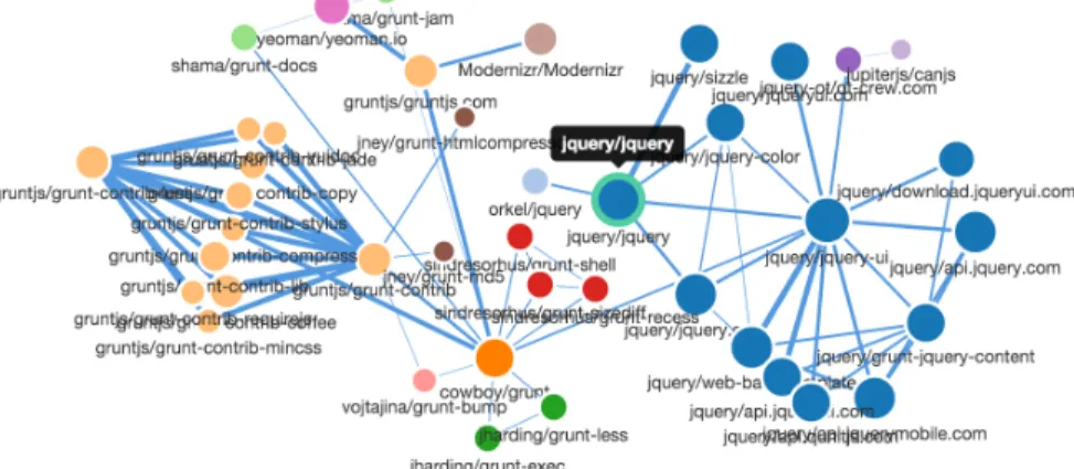
In our visualization, we let the size of the nodes be an indication of the popularity of the node, by using a logarithmic scale of the number of times the node occurs in the data set. The colors of the nodes are used to indicate which repositories have the same owner.

Figure 4.1.1: Example network graph. Collaboration network with depth 3 around the GitHub repository

jquery/jqueryon September 10th_{, 2012.}

Edges

In our model, network edges represent collaboration relationships. When a user commits to repository A and (some time later) to repository B, we can say that these repositories are connected by a relationship. However, since many repositories on GitHub are local forks (Kalliamvakou et al., 2014), we consider two repositories to be connected only when at least two users have recently contributed to both repositories. The same holds for relationships between users, for these we require at least two common repositories the users have recently committed to.

We use edge weights to indicate the number of a mutual contributions and the recentness of these contri-butions. I.e., the strength of the relationship between Aand B on a certain point in time is based on how recent the last contribution toAwas and how recent the contribution toB was.

When there has been no commit to eitherAorB in the last 30 days, we model the edge weight to be 0, i.e. the repositories are no longer connected. To do so, we define therecency of an eventeat a certain point in time as

recency(e) = max

1−number of daysewas ago

30days ,0

,

such that the recency is a number between 0 and 1, being 0 when the event was 30 days or more ago and 1 when the pull request just took place (and e.g. 0.5 when it was 15 days ago). The number of days can be a decimal number, e.g. 6 hours ago is 0.25 days ago.

(33)

edge weight(A, B) = X

all users

recency(last pull request of this user to A)·recency(last pull request of this user to B).

For edges in user-centered graphs, we use an analogous formula.

Example:

Consider a sample set with usersX andY and repositoriesAandB. Suppose

• userX made his last push (or successful pull request) to repositoryA 1 day ago and to repositoryB 2 days ago, and

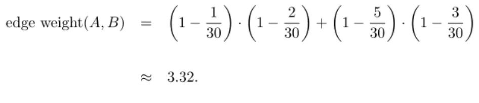
• userY made his last push or pull request to repositoryA 5 days ago and to repositoryB 3 days ago. Then edge weight(A, B) = 1− 1 30 · 1− 2 30 + 1− 5 30 · 1− 3 30 ≈ 3.32. Network

We aim to reconstruct networks around a given repository or user, which we call the origin node. I.e., starting from the origin node, we look for the software ecosystem of which it is part. Using our definition of edge weight, we can find nodes connected to the origin node. From there, we can find nodes connected to these nodes. We call the number of times this procedure is repeated thedepthof the network.

Figure 4.1.2: Repository-centered collaboration network with depth 2 around the GitHub repository

(34)

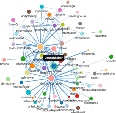
Figure 4.1.3: User-centered collaboration network with depth 3 around the GitHub user JosephSilberon September 19th_{, 2014.}

4.2 Data Collection

The data for our research is obtained from the GitHub Archive database, which contains historical public data from February 2011 until now. For the purpose of our research, we limit our scope of GitHub data to the years 2012, 2013 and 2014, three full years.

We choose to mine our data from the GitHub Archive rather than from GHTorrent since the GHTorrent data (currently) does not go back in history far enough (March 2012). Moreover, since we have to execute complex queries on the data set, we have to download the entire history of push events and pull requests during our scope period, for which we would have to download a 120+ GB database if using GHTorrent1_{. The same}

data can be downloaded in much smaller chunks from the GitHub Archive, from which the relevant data can be extracted, which is only 8.4 GB large when saved using MySQL in InnoDB compact row format2_.

Issues that arose during the mining process were:

• Data from the GitHub Archive project is stored in JSON3_{format, compressed using gzip}4_{and combined}

as one file per hour. These files are sometimes large to extract in-memory.

• The data files in some cases contain multiple JSON objects per line, which is slightly incorrect JSON and needs to be corrected before further processing.

1_{http://ghtorrent.org/downloads.html}

2_{See https://dev.mysql.com/doc/refman/5.7/en/innodb-row-format.html} 3_{http://www.json.org/}

(35)

• Timezones of dates differ per month (some are in UTC, others in PST with daylight saving in summer time), which has to be taken into account.

• During the scope period, the event structure changed a few times, because of introductions of new GitHub API versions.

• The useful mined data has to be stored in a local database, at the end of the mining process containing over 130 million rows of data.

All issues could be taken care of, resulting in an efficiently stored database table that functioned as a further basis for analysis. The 130 million rows of data were stored in an InnoDB table with a size of 8.4 GiB excluding indices.

4.3 Data Processing

The database query to identify ecosystem relationships from the dataset as described in Section 4.1 is relatively complex, especially since it identifies relationships for a period of time. In order to be able to execute this query efficiently, database indices help to reduce execution time and processing power. The trade-off is that extra storage space is required. In our case, an additional 8.5 GB of space was used for database indices.

The algorithm to identify ecosystem relationships as described above has complexity O t·nd+1

, where t is the number of days, n is the size of the data set, anddis the depth of the network we want to obtain. This algorithm is in general too complex to execute in real-time, therefore resulting ecosystems are stored in a database as well. Since a network of depth 2 contains the network of depth 1, the additional nodes and edges computed for higher degrees are stored in complement tables.

The code to collect the data and analyze it is stored as an open-source GitHub repository itself5.

4.4 Data Analysis

From the resulting networks, properties such as defined in Sections 3.3.1 and 3.3.2 can be measured for each moment in time. These network properties can be displayed as graphs.

As discussed in Section 3.4, size is the most suitable network property to observe as describing ecosystem life cycles.

(36)

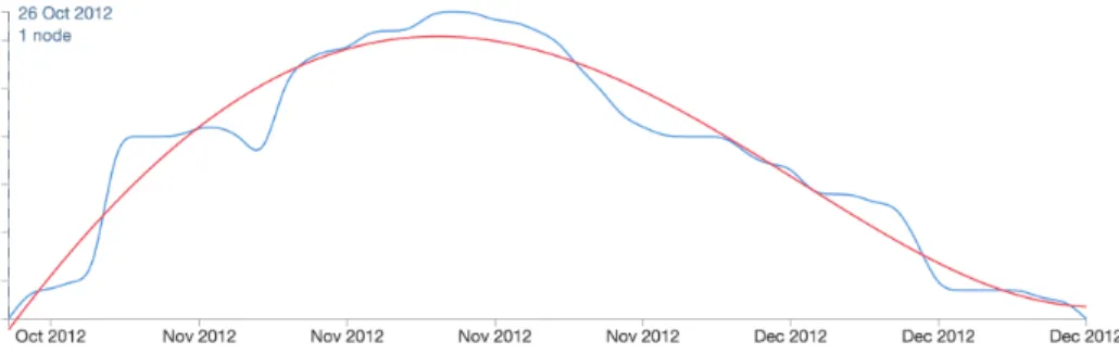
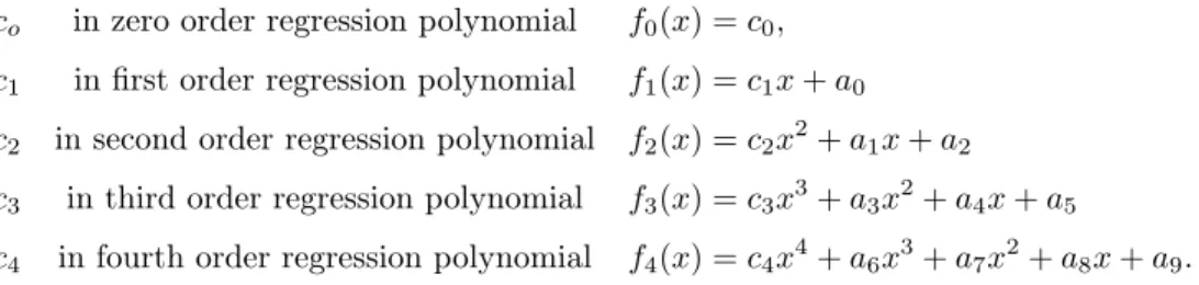
Figure 4.4.1: Size of the user-centered collaboration network with depth 3 around the GitHub useroszczep. The blue line indicates the ecosystem size on a day-to-day basis, of which the red line is the fourth order regression polynomial (discussed in the next chapter).

4.5 Results

The tool developed for our analysis can be viewed online6_{. Using our method, software ecosystems can be}

identified in an objective way. The resulting collaboration networks can be analyzed in detail.

The computation is not instant, but can be regarded to be relatively fast, taking into consideration the size of the data set. However, the complexity of the operation is an issue when trying to identify networks with a high depth. Computation time can be reduced by using indices, however requiring extra storage space. Our second research question was “How can collaboration in software ecosystems be measured and visualized, based on data from a public data source?”. Our model provides an acceptable method to do so, which is applicable to multiple definitions of software ecosystems. Key features of our model are:

• Based on co-authorship.

• Objective, no human input required, making it possible to analyze large numbers of collaboration networks.

• Suitable for longitudinal analysis.

• Balanced, keeping track of co-authorship for a sliding scale of time. • Relatively efficient.

• Storing data in a compact way by using complement tables.

• Aimed at GitHub, but suitable to extend to other software repository systems.

• Requiring relatively much storage space, mainly caused by the large number of events that take place on GitHub.

Evolution of Collaboration in Open Source Software Ecosystems