EXPLORATORY ANALYSIS OF HUMAN SLEEP DATA
by
Parameshvyas Laxminarayan A Thesis
Submitted to the Faculty of the
WORCESTER POLYTECHNIC INSTITUTE In partial fulfillment of the requirements for the
Degree of Masters of Science in
Computer Science January, 2004 APPROVED:
Professor Carolina Ruiz, Thesis Advisor
Dr. Majaz Moonis, Thesis Co-Advisor,
Director, Stroke Prevention Clinic, UMass Memorial Medical Center
Professor Sergio A. Alvarez, Thesis Co-Advisor, Boston College
Professor Matthew Ward, Thesis Reader
Abstract
In this thesis we develop data mining techniques to analyze sleep irregularities in humans. We investigate the effects of several demographic, behavioral and emotional factors on sleep progression and on patient’s susceptibility to sleep-related and other disorders. Mining is performed over subjective and objective data collected from patients visiting the UMass Medical Center and the Day Kimball Hospital for treatment. Subjective data are obtained from patient responses to questions posed in a sleep questionnaire. Objective data comprise observations and clinical measurements recorded by sleep technicians using a suite of instruments together called polysomnogram. We create suitable filters to capture significant events within sleep epochs. We propose and employ a Window-based Association Rule Mining Algorithm to discover associations among sleep progression, pathology, demographics and other factors. This algorithm is a modified and extended version of the Set-and-Sequences Association Rule Mining Algorithm developed at WPI to support the mining of association rules from complex data types. We analyze both the medical as well as the statistical significance of the associations discovered by our algorithm. We also develop predictive classification models using logistic regression and compare the results with those obtained through association rule mining.
Acknowledgement
The opportunity to write these few lines would not have materialized without the blessings of Amma, Appa, Mrs. Sampada Kaji and the guidance and support of my advisors and friends. Words I put down here cannot truly express my gratitude to Prof. Carolina Ruiz for taking me under her wing and guiding me in every possible way. Many thanks professor, for taking time out week after week to discuss my work and review the endless drafts of my reports and presentations. Several neurologists and doctors shunned from providing us sensitive data on patient’s visiting a sleep laboratory. I would like to express my deepest appreciation to Dr. Moonis for pushing to get the data released and agreeing to discuss with me issues at times in-between clinic appointments. My experimental results would not have been the same without the help and guidance of Prof. Sergio Alvarez. Many thanks Prof. Sergio for all your advice in logistic regression and obtaining of statistically significant association rules. I would also like to thank all my friends at WPI for their support and encouragement during my thesis. Special thanks to Abhishek, Mitesh, Aditya, Roshan, Nitin, Kalyan and Sidharth for literally going out of your way in helping me reach UMass Medical Center or Day Kimball Hospital on very short notices. Thanks guys!!
Contents
1 Introduction 10
1.1 Domain overview . . . 10
1.2 Need for computational analysis on collected data . . . .10
1.3 Standardized procedure for sleep scoring . . . .11
1.4 Knowledge discovery using data mining . . . 12
1.5 Context of this research. . . 13
1.6 Problem statement . . . .14
1.7 Thesis contribution . . . 14
1.8 Application areas. . . 15
1.9 Summary. . . .16
2 Background 18
2.1 Instrumentation and signal processing . . . 18
2.2 Sleep stage scoring and their interpretation. . . .19
2.3 Sleep disorders . . . 21
2.4 Waikato environment for knowledge analysis - WEKA . . . 21
2.5 Mining association rules over transactional data. . . .22
2.6 Mining association rules over complex data . . . 26
2.7 Additional statistical measures for association rules. . . .26
2.8 Logistic regression . . . .28
2.9 SAS – statistical software package . . . .30
2.10 Summary. . . 31
3 Review of Related Literature 33
3.1 Mining over questionnaire data . . . 33
3.3 Inductive learning for sleep stage classification . . . 34
3.4 Influence of papers reviewed in developing our approach. . . 35
3.5 Summary. . . 36
4 Our Data Analysis Approach 37
4.1 Association rule mining with time sequences . . . 39
4.2 Event identification using filters . . . 40
4.3 Limitations in association rule mining with relative time . . . .41
4.4 Temporal association rules using time windows . . . .41
4.5 Contribution of our approach . . . 46
4.6 Summary. . . 46
5 Macro-level: Dataset Description and Analysis 48
5.1 Macro-level dataset details . . . .48
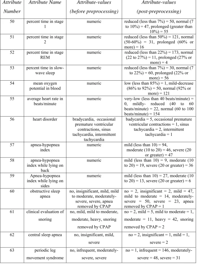
5.2 Pre-processing of macro-level dataset. . . .49
5.3 Analysis of macro-level data. . . .55
5.4 Summary of results . . . .66
6 Micro-level: Dataset Description and Analysis 68
6.1 Dataset details . . . 68
6.2 Pre-processing of micro-level dataset. . . .70
6.3 Dataset organizations . . . .72
6.4 Analysis of micro-level data . . . 73
6.5 Summary of results. . . .88
7 Mixed-level: Dataset Description and Analysis 90
7.1 Dataset and pre-processing details. . . .90
7.2 Analysis of mixed-level data. . . .90
7.3 Differences between association rule mining and logistic regression . . . .146
7.5 Summary . . . 161
8 Conclusions and Future Work 163
8.1 Conclusions . . . .163
List of Figures
4.1 Organizing data into macro, micro and mixed-level datasets . . . .38
4.2 Relative time variation of stage-2 and REM . . . .40
4.3 Building windows from epochs (Window = 3 epochs = 90 seconds) . . . .42
4.4 Building windows from epochs (Window = 5 epochs = 150 seconds) . . . . .43
4.5 Filters for transforming raw sequence data into set-valued with information on the windows within which events are witnessed along with the frequency of event-fragmentation . . . .44
4.6 Statistically robust rule obtained from micro-level dataset . . . 46
5.1 Block diagram of macro-level dataset structure . . . . 49
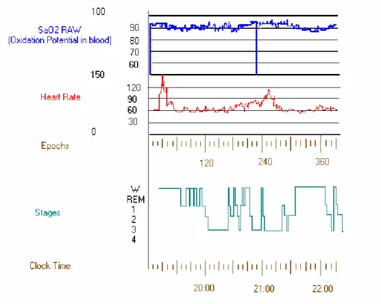
6.1 Variations in recordings from polysomnogram instruments . . . 70
6.2 Variation in stage-2 and REM correlating with low heart rates and low oxygen potential. . . 86
7.1 Frequent windows of below baseline oxygen potential that correlates with mild to moderate OSA. . . 100
7.2 Epoch windows of 20 with low baseline oxygen potential and low heart-rate that correlate with moderately severe OSA. . . 103
7.3 Epoch windows of 20 with low baseline oxygen potential and low heart-rate that correlate with mild OSA. . . 104
7.4 Variation of stages 2 and REM of sleep in patients suffering from moderately severe and mild obstructive sleep apnea (OSA) . . . 107
7.5 Most frequent windows of stages 2 and REM sleep noticed in patients having moderate depression. . . 111
7.6 Most frequent windows of stage 2 and REM sleep noticed in obese patients having mild to moderate depression. . . .113
7.7 Most frequent windows of stage 2 and REM sleep noticed in obese
patients having mild to moderate epworth indices. . . 115 7.8 Most frequent windows of stage 2 and REM sleep noticed in female
patients having overweight and obesity complaints. . . 117 7.9 Most frequent windows of stage 2 and REM sleep noticed in male
patients with moderate epworth ratings. . . .118 7.10 Most frequent epoch windows with stages 1,2 and REM noticed in
patients who exercise 3-5 times/week. . . 122 7.11 Most frequent epoch windows with stages 1,2 and REM noticed in
patients who do not exercise at all. . . 123 7.12 Most frequently witnessed windows of stages 1,2 and REM in patients who
do not drink caffeinated beverages and those who have little amounts of it each day. . . 125 7.13 Sleep-efficiency variations with stages 1,2 and REM . . . .128 7.14 Most frequent epoch windows of stages 1,2 and REM of sleep that correlate
with sleep latency till stage 1, sleep latency till REM and sleep efficiency.130 7.15 Variations in stages 1,2,3,4 and REM correlating with male and female
patients with varying exercise habits. . . 134 7.16 Correlation between stages 1, 2, 3, 4, REM of sleep with varying degrees
of OSA . . . .138 7.17 Correlation between mild-OSA and sleep stages observed with
window-size = 25 epochs. . . 141 7.18 Correlation between moderately severe OSA and sleep stages observed with
window-size = 25 epochs. . . 142 7.19 Variations in stages 1, 2 of sleep and OSA influencing sleep efficiency. . .145
List of Tables
2.1 Simplified outline of the R&K sleep scoring criteria based on
polysomnogram signals . . . 20
2.2. Dataset with instances representing customer transactions . . . 23
5.1 Macro-level dataset before and after pre-processing. . . .54
5.2 Miniature snapshot of macro-level dataset.. . . .55
6.1 Attribute values and their events of interest . . . .71
6.2 Events based on oxygen potential value ranges . . . .71
6.3 Events based on heart rate value ranges . . . .72
6.4 Epoch-based dataset organization . . . .72
Chapter 1
Introduction
1.1Domain overview
Though it is a very common behavior, sleep is an extremely complicated domain to study because of the large number and diversity of factors influencing it. Sleep is a dynamic phenomenon with the interplay between several factors continuously affecting it. This interplay has a direct influence on the mental and physical well- being of the individual and exhibits a high correlation in inducing sleep related disorders. A full understanding of sleep, therefore, requires disentangling the complex psychological, demographic and behavioral factors that have a direct bearing on an individual’s sleep. Determination of the factors affecting sleep has come about after years of study by several behavioral scientists, psychologists, medical professionals and biomedical engineers. Sleep experts with the aid of the factors identified as important have successfully provided valid explanations to several of the phenomena noticed during sleep. However, there are several other interesting facets that if explored, will prove to be interesting and possibly useful to the sleep research community.
1.2Need for computational analysis on collected data
Exploratory analysis in any domain requires accumulation of large amounts of data. The domain of sleep analysis is no exception to this. With the increase in the amount of data for analysis, use of computational techniques becomes possible. Today, due to the advent of powerful computational tools and models, the sleep domain is turning out to be a prime area of investigation in computational research in biological systems.
The initial sleep studies concentrated on finding the various emotional and physical traits of individuals that bear an influence on sleep. However, in the last three to four decades, due to rapid advances in electronic instrumentation and technology, reliable and accurate measurement of electronic signals along with storage and retrieval of large volumes of data has become particularly easy. This development has encouraged scientists to utilize the recordings made by several electronic devices to obtain a better understanding of the complex processes and transformations in vital body processes that occur during sleep. This procedure inevitably leads to the collection of large amounts of data that needs to be analyzed to provide any kind of informed judgment. This is where, computational techniques and algorithms used primarily in data mining and machine learning come into play.
1.3Standardized procedure for sleep scoring
As mentioned earlier, the improved accuracy and interpretability of electronic instrument readings led to their use in numerous areas. Hence, several instruments for measuring physiological behavior were used by researchers to help interpret the various intricacies of sleep. Researchers were using recordings from several instruments to classify sleep into different stages. However, since no strict standard was being followed or maintained on the devices and the recordings that need to be analyzed, it became difficult to interpret the results produced by different researchers. A change was brought about after the Association for the Psychophysiological Study of Sleep (APSS) appointed a committee of sleep researchers to develop a standardized system to score sleep into different stages. Two sleep researchers, viz., Rechtschaffen and Kales (henceforth R&K) brought forth a model that took the help of the measured readings from a few electronic instruments as well as visual interpretation of features by technologists during the night under observation to classify sleep into different stages [RK68]. The model also called R&K model divides a normal sleep into six stages: five stages of sleep (sleep stages 1-4 and Rapid Eye Movement, or REM sleep) plus periods of wakefulness. Variations in the sleep stages lead to different sleep patterns. The suite of instruments whose combined tracings help in sleep stage classification are together called Polysomnogram.
Polysomnogram comprises instruments used to record the brain activity by measuring electric potentials in the brain using an Electroencephalograph (EEG), electric potential output caused by movement of body parts using an Electromyograph (EMG), and the electric potentials resulting from eye movements through an Electro-oculograph (EOG). In most cases, additional equipment to keep track of breathing and the amount of oxygen in the patient’s bloodstream is also used. Every thirty-second of polysomnogram recording is classified into one of the six sleep stages based on the R&K classification model. The thirty second window of sleep that is classified is called ‘epoch’.
1.4Knowledge discovery using data mining
In this thesis we concentrate on applying a computational technique that is widely used in the field of Data mining to analyze sleep. Data mining is a branch of Knowledge Discovery in Databases (KDD), which elicits knowledge or information from data stored in large data repositories. It uses techniques that can help in extracting interesting and novel patterns from the data.
Data mining is a multidisciplinary field greatly influenced by a number of fields including artificial intelligence, machine learning, statistics, databases, visualization, and pattern recognition. The algorithms implemented in data mining utilize principles, proofs and deductions from all these fields. They are of great help in exploratory data analysis and in predictive classification type of problems. Deciding as to which data mining technique needs to be applied depends largely on the nature of the dataset, the type of problem being attempted and the interpretability of the results generated.
A technique often used in the field of data mining to perform exploratory data analysis is association rule mining. The idea behind the use of association rule mining is to be able to state with suitably high accuracy that presence of certain attribute value conditions lays the seed for presence or observance of certain other attribute conditions. For instance, moderate to high depression in patients complaining of excessive daytime sleepiness is indicative of very low sleep efficiency. In this case, the values for attributes,
viz., depression and excessive daytime sleepiness lay the seed for observing low sleep efficiency levels. Another motivating factor in using this approach was the fact that, there is very little research material available on past work done in mining associations over sleep data.
1.5Context of this research
As part of the treatment of people suffering from sleep disorders, physicians evaluate their mental and physical state of health. Towards this end patients are required to fill in a questionnaire when they visit the sleep laboratory (refer to Appendix-A for the sample questionnaire). The questionnaire requires the patient to reveal among other information their demographic details, the nature of sleep disorders they suffer from, other disorders or diseases they have or are suffering from, their food habits, behavioral habits etc. Following this, the patient undertakes a sleep test.
Based on the initial assessment, there are different sleep studies that the physician may recommend. The more common laboratory studies are the all-night polysomnogram study and split-night study. Normally, the all-night polysomnogram study is recommended for patients who have a suspected sleep disorder. For patients suffering from or suspected of suffering from sleep apnea (most common sleep disorder), a Split-night study is generally recommended. During the Split-night of the test, the technicians monitor the patient’s progress into sleep. In the event of severe apneaic episodes, they put the patient under CPAP (continuous positive airway pressure). Following the night under observation, sleep stage classification as per the R&K model is performed using the polysomnogram readings and the technician’s interpretations of the patient’s sleep. The technician also prepares a report summarizing the patient’s sleep trends during the night of study. This summary report aids the physician in making a diagnosis.
The dataset used for analysis comprises subjective and objective information collected from the epoch-by-epoch polysomnogram recordings, questionnaire responses and the summary report created by technicians for every patient.
1.6 Problem statement
Our motivation to perform this analysis is dual fold. Firstly, we aim at capturing relationships of significance among the several factors considered. We are more interested in finding if a particular demographic attribute or factor correlates highly with a certain sleep behavior or disorder. For example, patients having high Body-mass index (i.e., patients who are overweight or obese) are more prone to snoring while asleep. This is pretty obvious pattern noticed in patients whose Body-mass index exceeds the normal range. A more interesting result though is ascertaining that increasing levels of depression do not influence Periodic Leg Movements (PLMS), a very common sleep disorder. In other words, the degree of depression a patient suffers from cannot be used as a marker for diagnosing PLMS. Secondly, we are also interested in obtaining relationships linking sleep pattern variations with susceptibility of patients to suffer from disorders or diseases. To achieve these twin objectives we rely on association rule mining.
1.7 Thesis contribution
Currently, the most commonly used approach for analyzing data from medical domains is the use of statistical techniques. One of the major contributions of this thesis is to introduce and demonstrate by way of experimental results that techniques from the field of data mining are richer in the quantum of information that they provide following data analysis in comparison with statistical techniques that are currently in vogue. Also we highlight the advantages of association rule mining over statistical techniques like logistic regression when it comes to exploratory data analysis. This thesis also demonstrates different ways of data organization to counter the non-homogeneity of data and perform analysis to extract useful information.
The traditional association rule mining algorithm [AS94] can only handle data that can be represented in categorical or numeric forms. Former and current students at WPI have worked on extending this system to support more complex data formats such
as sets [Shoe01, Stoe02] and time sequences [Pray02]. In this thesis, we conduct experiments by representing data as both time sequences and sets by writing special filters to capture events of interest that occur during the different epochs of the patient’s sleep. We also describe the window-based method of data transformation and organization that transforms the raw time-sequence attribute values to a form where attribute values with real-time information and occurring within the same window are placed in the same set. This system helps in providing more information as part of the rules. This aids the domain expert to obtain greater insight into the patient’s sleep progression, which in turn helps in making a more accurate or reliable prognosis.
1.8 Application areas
The initial impetus to initiating this project was to develop systems that would find use in the area of Untethered healthcare and Patient monitoring. We believe that by including a diverse set of patients suffering from other disorders or pathological conditions and with more research it is possible to develop early detection systems purely on the basis of monitoring the patient’s sleep and responses to questionnaires that elicit the necessary demographic and behavioral details. This is especially significant in the light of the fact that today pathology detection is mostly symptom-driven. Our models for detection of pathology are not symptom-driven. Instead they are based on subjective and objective information gathered from patients visiting the sleep laboratory. This will facilitate screening of patients visiting physicians with any complaints and short-listing likelihood of pathologies they might be suffering from. Thus, in addition to early detection, it can probably even serve to pre-empt occurrence of other pathologies. The models could also be embedded into devices designed to monitor patients during the night of sleep and relay the information to a central repository or emergency units, thus providing untethered healthcare services.
1.9 Summary
In this chapter we provide the overview of how research in human sleep has evolved from subjective behavioral assessments initially to introduction of objective measures with the advancement of technology over the past several decades. The suite of electronic instruments used to collect data from observing the patient during sleep is called Polysomnogram.
There are plenty of interesting associations and relations, which would enormously benefit the researchers in this field. Past attempts have involved abundant use of statistical techniques to dig out these relations. Our emphasis will be on use of association rule mining to extract novel and interesting patterns from the data collected. We are particularly interested in patterns relating sleep variations with degrees of pathology. Also, domain experts view with interest rules that can establish relationships among demographic, behavioral and clinical factors considered in the analysis.
The dataset for this thesis comprises the questionnaire responses of patients visiting a sleep laboratory in addition to the measurements made by polysomnogram instruments and the summary report compiled by technicians. Data collection was not easy since information was spread over two locations. As a result, we were unable to obtain all information that was originally intended for most patients. We attend to this problem by modifying our datasets for analysis accordingly.
This thesis shows that medical experts can rely on techniques used in data mining instead of purely statistical techniques for data analysis. It demonstrates that association rules are more informative than logistic regression, a technique used widely for medical data analysis. The thesis also introduces the concept of mining for association rules within user-specified windows in real-time to obtain rules with more information content.
With further research, results obtained from experiments performed during this thesis will find applications in the area of untethered healthcare and remote patient
monitoring. Medically relevant and strong rules can perhaps in the near future also lead to pre-emptive treatment for several pathological disorders.
Chapter 2
Background
2.1 Instrumentation and signal processing
Amongst all the polysomnogram instruments in use today, the EEG was the first to be used to analyze human sleep. The earliest description of the use of EEG to analyze sleep appears in the paper chronicling the work done by Loomis et al. [LHH36]. With the exception of REM, all other stages of sleep were distinguishable with the help of measurement logs obtained from EEG records. It was not until the addition of the EOG as another device to analyze sleep that REM stage identification became possible [AK53]. EOG, which detects the electro-potential difference between the front and back of the eye, is able to identify the REM stage, which is characterized by repeated bursts of rapid eye movement. Later, researchers found that EMG provided a more reliable marker for detection of REM than just the presence of bursts of rapid eye movements [CR94]. EMG is a device used to measure muscle tension using the surface electrodes placed over the chin. Also EMG electrodes placed over the skin on either leg pick up movement of legs during sleep. R&K conceived their sleep stage classification model on the basis of the collective experience and results of numerous researchers targeting similar goals.
Polysomnography was first used to detect sleep irregularities at Stanford University during the 1970s. Polysomnography combines tracings from respiratory and cardiac sensors together with EEG, EMG and eye movement recordings to partition sleep into different stages [But96]. EEG is a multi-dimensional signal recorded using an array of electrodes placed at different locations on the scalp. The EEG electrodes are placed over the central and occipital areas of the brain in accordance with the international 10-20 system (C3 or C4 and O1 or O2) [Jas58]. EOG electrodes are placed in the vicinity of the right and left outer canthus (canthus- the angular junction of the eyelids at either corner
of the eyes). EMG electrode is fixed over the chin to trace muscular variations. The EMG electrode placed over the skin surface on the leg captures leg movements. The raw signals derived from the sleep patient have extremely low voltages and are highly susceptible to electrical interference. The electrical background activity of the human brain is in the range of 1-200uV, while the Evoked Potentials (EP) have an amplitude of only 1-30uV[BS90]. Many techniques have been adopted to keep the amount of electrical interference to a minimum. One of the measures for instance is selecting high quality electrodes. However not all artifacts are easy to be contained or minimized. Artifacts resulting due to movement of the patient while asleep make signal processing complicated.
2.2 Sleep stage scoring and their interpretation
Every thirty-second piece of a sleep recording constitutes an epoch. However, for specific research experiments epochs with smaller magnitude have also been used. Sleep stage scoring involves classifying the polysomnogram signals on an epoch-to-epoch basis. Epochs are scored into sleep stages in accordance with the R&K model. Sleep staging is guided by the frequency of the waves recorded by the polysomnogram instruments. Among the various polysomnogram instruments, R&K relies most on the EEG recordings to aid in staging. The EEG frequency bands used by the R&K model for staging sleep are mentioned below:
Alpha Rhythm: 8 to 13 cycles per second or cps Beta Rhythm: more than 13 cps
Delta Rhythm: less than 4 cps Theta Rhythm: 4 to 7 cps
Table 2.1 below gives the outline of the R&K model for sleep staging using polysomnogram data.
Stage/Stage EEG EOG EMG Relaxed Wakefulness Eyes closed: alpha (8-13cps)
Eyes open: lower voltage, mixed frequency Voluntary control; REMs or none; blinks; SEMs* when drowsy Voluntary movement; tonic activity relatively high
Stage 1 Relatively low voltage, mixed frequency
Maybe theta (3-7 cps) activity with greater amplitude
SEMs Tonic activity, maybe slight decrease from
waking Stage 2 Relatively low voltage, mixed
frequency.
Presence of sinusoidal waves (sleep spindles) 12-14 cps. Presence of negative sharp wave followed by slow positive component (K-complex) for time ≥ 0.5 sec
Occasional SEMs
Tonic activity, low level
Stage 3 ≥20 ≤ 50% high amplitude (>75 µV), slow frequency (≤ 2cps)
None, picks up EEG
Tonic activity, low level
Stage 4 >50% high amplitude, slow frequency
None, picks up EEG
Tonic activity, low level REM Relatively low voltage, mixed
frequency, sawtooth waves, theta activity; slow alpha
Phasic REMs Tonic suppression
Table 2.1: Simplified outline of the R&K sleep scoring criteria based on polysomnogram signals (Modified from Chapter 15, Page 1202, [CR94]).
2.3 Sleep disorders
The more common of the numerous sleep disorders afflicting patients include narcolepsy, insomnia, excessive daytime sleepiness (EDS), snoring, periodic leg movement syndrome and sleep apnea. Sleep apnea is perhaps the most commonly diagnosed sleep disorder. This disorder has quite a few variants, which have been studied closely due to their common occurrence. Sleep apnea is a disorder where the patient experiences difficulties in breathing for several seconds during sleep. Based on the degree of inconvenience, we find physicians diagnosing patients with the different variants of sleep apnea. Hypopnea, for instance, is the condition where patient can breathe with some amount of effort and difficulty (can vary from person to person from mild effort to concerted effort) for several seconds during sleep. Obstructive sleep apnea on the other hand, is the case when the patient completely fails to inhale for several seconds during sleep. Of the different variants, Obstructive Sleep Apnea or OSA is found to be the most predominant form of sleep apnea affecting people.
2.4 Waikato environment for knowledge analysis – WEKA
For the mining task we seek the services of an open source machine learning suite called WEKA (stands for Waikato Environment for Knowledge Analysis). WEKA comprises of a collection of machine learning algorithms catering to different data mining applications and domains [FW00]. Being open source software, not only is it possible for users to utilize the various machine learning algorithms to perform different experiments but also suitable for developers to extend the algorithm functionality to build different applications. At WPI, students have worked on optimizing the execution of the association rule mining algorithm and extended it to handle other more complex data formats such as set-values [Sho01, Sto02] and time sequences [Pra02].
2.5 Mining association rules over transactional data
Association rule mining is used to extract interesting correlations from datasets having several data items. The discovery of interesting associations and relationships among data items in large sets of data helps analysts and managers enormously during the decision making process [AS94]. The original motivation for and the implementation of association mining algorithms were more applicable to providing solutions in business domains. In this thesis, we attempt to gain its benefits by applying it over the medical domain.
We now explain briefly a few important points relating to the functioning of association rule mining. Every variable or attribute-value pair that forms part of the dataset is called an item. A set of items is referred to as an itemset. Association rule mining employs two basic measures to extract interesting relationships between itemsets (set of one or more items) in a dataset. The two measures are called support and confidence.
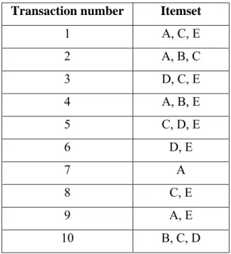
To explain the terms and measures used in association rule mining, we introduce an example. Consider the dataset to represent the transactions of individual customers visiting a store. Each row of the dataset comprises any combination of items (‘A’, ’B’, ‘C’, ‘D’ and ‘E’) indicating the set of items purchased by each customer during a single transaction. Each row is referred to as an instance of the dataset.
Consider the dataset comprising ten instances as shown in Table 2.2. Each instance indicates the set of items or itemset purchased by the customer from the store. Consider also the rule A & B Î E. This rule states that the presence of A and B in an instance makes it likely for E to also occur in the instance. This likelihood is measured by the Confidence of the rule. Confidence informs us as to how frequently the consequent of
the rule (in this case, itemset Y = {E}) appears along side the antecedent (in this case, the itemset X = {A,B}) among the instances forming the dataset. The Support for a rule is the
Transaction number Itemset 1 A, C, E 2 A, B, C 3 D, C, E 4 A, B, E 5 C, D, E 6 D, E 7 A 8 C, E 9 A, E 10 B, C, D
Table 2.2. Dataset with instances representing customer transactions
Mathematically these measures may be expressed in terms of a probability relationship as,
The Apriori algorithm [AS94] is the standard algorithm to mine association rules. The apriori algorithm is a two-stage process.
Stage1 consists of finding all frequent itemsets and
Stage2 consists of generating rules from the frequent itemsets.
The input to the association rule mining algorithm is the dataset to be mined together with thresholds of minimum confidence and minimum support that the rules output must satisfy. In other words, the rules output by the system will all have confidence and support values equal to or above the user-specified values of confidence and support.
2.5.1 Generating frequent itemsets
The apriori algorithm is based on the Apriori principle [AS94] for generating frequent itemsets. An itemset is considered frequent if the ratio of the number of instances in which it appears to the total number of instances in the dataset (i.e., the support of the itemset) is equal to or greater than the minimum support threshold value specified by the user. The Apriori principle states that all subsets of a frequent itemset must also be frequent.
The Apriori algorithm constructs the frequent itemsets level by level. On level1, it constructs all frequent itemsets of cardinality 1. On level2, it constructs all frequent itemsets of cardinality 2 and so on. Apriori assumes that the itemsets are arranged in lexicographic order. Joining of two itemsets at one level to generate the itemset of the next higher level takes place only if all the items save for the last item in the two itemsets are alike. For instance, consider two itemsets at level-3, C1 and C2 that have only the last
item in the itemsets different. C1 = {c11, c12, c13};
C2 = {c21, c22, c23}
The condition c13 < c23 ensures that the two itemsets being joined are not duplicates and
helps maintain the lexicographic order while performing the join [HK00]. The new itemset obtained is one level higher. In this example, the itemset generated is of level-4. Let us name it itemset M. We observe that,
M = {c11, c12, c13, c23} is the itemset resulting from the join between C1 and C2.
On the new itemset generated by the join, the prune step is employed. This step verifies whether the Apriori condition holds true for the new itemset. It checks if all the subsets of the newly formed itemset are frequent. If this is not found to be true, the new itemset generated during the join is pruned. In the example under consideration, the level-4 itemset M has level-4 level-3 subsets.
M11 = {c11, c12, c13}; M12 = {c11, c12, c23}; M13 = {c11, c13, c23}; M14 = {c12, c13, c23}
Each of these subsets, viz., M11, M12, M13 and M14 must be frequent for itemset M to be
possibly frequent. Whether the itemset M is frequent or not is determined by counting the actual support of the itemset M by going over every instance of the dataset.
2.5.2 Rule generation process
Following the generation of frequent itemsets, we enter the second stage of association rule mining, which is rule generation. Our objective is to generate strong association rules that satisfy the thresholds of minimum support and minimum confidence specified by the user. As mentioned earlier, confidence for a rule X → Y is the ratio of the number of instances in the dataset containing X that also contain Y. The same can be expressed as,
We use equation (3) over the generated frequent itemsets to obtain rules with acceptable levels of confidence as follows.
For each frequent itemset M
For each possible subset, S of M
We calculate the confidence of the rule, (M-S) → S using equation (3).
If the value of ‘r’ is greater than or equal to the minimum confidence
threshold set, then the rule, (M-S) → S is output together with its confidence and support values.
2.6 Mining association rules over complex data
The traditional association rule mining algorithm supports only a limited number of data formats that are more common in market-basket datasets and similar transaction-related domains. The data items normally are numeric or categorical in nature. For complex datasets having attributes that hold a set of items or time-series data, a modified version of the Apriori algorithm is required to perform the mining process. We explain in detail the modifications performed to extend the system to mine with more complicated data formats in section 4.1.
2.7 Additional statistical measures for association rules
One of the strengths of association rule mining is that it extracts all associations existing in the dataset that satisfy the user-specified minimum support and minimum confidence levels [LHM99]. This strength could also turn out to be a disadvantage since more often than not, the resulting set of rules is very large and analyzing them can become difficult. This is especially true in the case of data sets with several highly correlated attributes. Another problem that is often noticed is that we obtain rules with very high confidence values even though the attributes forming part of these rules are actually independent. To identify and thereby prune such faulty associations another
measure called ‘lift’ is used. For an association rule of the form X → Y, lift can be mathematically expressed as,
The lift provides a value that helps in understanding the extent of association or dependence the consequent attribute-values have on the antecedent attribute-values that form part of a particular rule. This in turn helps in evaluating the interestingness of a rule. Rules indicating high dependence of the consequent values on the attribute-values that make up the antecedents are considered particularly interesting. High attribute-values of lift are indicative of highly dependent and hence interesting rules. Lift values closer to zero are characteristic of weak associations between the antecedent and consequent attributes with low confidence. Value of lift close to 1 is indicative of the consequent occurring virtually independent of the antecedent. Rules with high confidence and lift values hovering around 1 are indicative of the fact that the association between the antecedents and consequents may have occurred by pure chance, since the consequent occurs roughly to the same proportion when considered in isolation.
Using values of confidence, support and lift it is possible to estimate the statistical significance of the generated rules by performing the chi-square test for independence and correlation [Alv03]. Pearson’s chi-square test is based on the comparison between the observed and the expected frequencies (counts). The chi-square statistic is the sum of the squares of the differences between the observed and the expected frequency. The statistic can also be calculated using observed proportions provided the total number of subjects (and hence frequencies) is known. In our case, since we know the total number of instances in the dataset, we make use of the three proportional measures confidence, support and lift to determine the chi-square value as mentioned earlier.
Below, we illustrate how the method introduced in [Alv03] of calculating the chi-square statistic using the three measures of confidence, support and lift helps in determining the interestingness of a rule. Consider, for instance the association rule,
The above rule indicates that there is a correlation between the attributes X and Y. We are trying to ascertain the statistical validity of the association given by this rule using the chi-square test. Using the technique specified in [Alv03] and the values of confidence, support and lift specified for the rule above, we arrive at a chi-square value of 84.6. Consulting the chi-square look-up chart for 2x2 table with 1 degree of freedom, we find that the value corresponds to a significance level that is better than 0.001. In other words, the value indicates that there is 1 in 1000 chance that the correlation exhibited by X and Y in the association rule occurs by chance. This indicates that the rule is represents a true association between X and Y and that it is statistically robust.
2.8 Logistic regression
Logistic regression is a statistical technique that is used widely for analyzing results from clinical and laboratory tests or trials in the medical domain. An English scientist, Francis Galton developed the technique of regression analysis in the 19th century. Logistic regression is a specialized version of simple regression analysis.
Regression analysis is used in predicting value of one variable (also called dependent variable) using values from one or more other variables (also called independent variables). It helps in determining the accuracy with which the independent variables predict the dependent variable. Further, regression analysis can also help in assessing whether a particular relationship is statistically significant. In other words, whether the relation obtained in a small sample is also seen in an entire population. The dependent and independent variables may hold numeric or categorical data values. Ordinary regression analysis, however, has an important limitation. It requires the dependent variable to hold continuous values. Logistic regression, on the other hand, can handle discrete-valued dependent variables.
Generally, in many applications where logistic regression is applied, the dependent variable takes only two values. The two values represent either presence/ absence of a condition or true/false type of responses. For these applications the logistic
regression applied is referred to as dichotomous or binomial logistic regression. There may also be applications where the dependent variable may take more than two values. Logistic regression applied on such datasets is referred to as multinomial logistic regression.
The independent variables in logistic regression may have numeric or categorical values. The logistic regression makes no assumption of the distribution of these variable values. Another advantage with logistic regression over regression is that the fitted regression co-efficients maintain probabilities within (0, 1) range rather than values, which could stretch between (-∞, ∞) in case of regression. This is achieved by log-odds transformation leading to a model given by the expression as described in [ED96],
p = probability of the dependent variable assuming a particular value, n = number of independent variables.
β0, β1, .., βn = regression co-efficients,
x1, x2, ..., xn = independent variables.
The regression co-efficients are estimated using the method of “maximum likelihood”. The response variable is assumed to have a binomial distribution.
The problem of establishing a relationship between the dependent variable and the set of independent variables ultimately boils down to identifying the subset of the latter having the greatest influence in determining the former. In logistic regression, deciding
whether a variable must enter the model or be removed from it is based on the chi-square statistic.
2.9 SAS – statistical software package
A number of statistical software packages are available today to perform analysis over the data. We make use of the UNIX SAS version 8.1 available at WPI to perform the logistic regression experiments. This version has a graphical environment for performing all necessary tasks over the data. Most of the manipulation, analysis of the data and plotting of the graphical output can be performed by using the pull-down menus from the windows that appear when SAS is activated. We could alternately write SAS programs to perform the different tasks. Typical SAS programs comprise of DATA step and several PROC steps for analysis. DATA step is used to load all the observations that form part of the dataset. Once the data has been read into the SAS dataset, SAS procedures are activated by the PROC step to analyze the data [ED96].
The weighted independent variables along with the regression co-efficients are used to estimate the response or dependent variable. SAS uses statistical measures to estimate the fitness of the model. The Akaike’s information criterion (AIC) [Aka74] and the Schwartz’s criterion (SC) are used to assess competing models. The two measures strive to select the most parsimonious model by balancing the fit against other factors [ED96]. Lower values of AIC and SC indicate more preferred models.
There is a third term, –2log L = -2Σlog(pj), where pj are the predicted values
obtained by replacing the β terms in equation (7) with estimated values.
The statistical measures to gauge model fitness lead us to test the validity of the hypothesis that says that all regression co-efficients of the model have a value that equals zero. We make use of chi-square to test if any of the independent variables has an influence on predicting the dependent variable.
The ‘Maximum Likelihood Estimates’ section of the SAS output provides us with calculated statistical values of the standard error, chi-square results and probability values of the explanatory variables in order to determine whether the hypothesis is true (i.e., whether the regression co-efficients take a value other than zero).
SAS also provides us with four measures to assess the predictive ability of the model selected. These are Somer’s D, Gamma, Tau-a and c. Higher the values of c, D, Gamma and Tau-a better is the predictive power of the model.
2.10 Summary
Polysomnogram is a suite of instruments used to measure physiological parameters of different body functions during patients sleep. It includes the Electro-encephalogram (EEG), Electro-oculogram (EOG), Electro-myogram (EMG) besides other instruments like the one to measure the oxygen potential in the patient’s bloodstream.
Staging of sleep is performed on the basis of the R&K model of sleep stage classification. It primarily uses the frequency of the EEG signals and the subjective interpretation of the technician’s observations during the night under observation to classify the patient’s sleep.
Some of the common sleep disorders are narcolepsy, obstructive sleep apnea, hypopnea, insomnia and periodic leg movement syndrome. The majority of patients reporting sleep disorders suffer from obstructive sleep apnea (OSA) in which the patient struggles to breathe for several seconds or minutes during sleep.
Association rule mining was designed and developed to be more suitable for data analysis over business domains. However, since they extract correlations between the various attribute-values considered, it is widely used in exploratory data analysis. Association rule mining generates rules from frequent itemsets based on two measures
called support and confidence. At every level frequent itemsets are generated in accordance with the Apriori principle. The principle states that all subsets of a frequent itemset need to be frequent. Rules output by the mining algorithm have support and confidence values equal to or above the user-specified minimum threshold values. We use the WPI-WEKA system for mining association rules. We determine the strength of the resulting associations by calculating the lift for the rules. To prune associations occurring due to pure chance, statistical robustness of rules is evaluated using the chi-square test for statistical significance.
Regression is a technique used to predict a dependent variable based on values taken by several participating independent variables. Ordinary regression analysis imposes the constraint that the dependent variable carries only continuous values. Logistic regression on the other hand supports cases where the dependent variable carries discrete values. Another advantage of logistic regression is that the regression coefficients are fitted to have probabilities within the (0,1) range. Logistic regression uses chi-square testing to determine correlations between the independent variables and the dependent one. Logistic regression experiments in this thesis have been carried out using the SAS statistical package.
Chapter 3
Review of Related Literature
3.1 Mining over questionnaire data
Mining over questionnaire data is not always straightforward. There are several reasons for this. One of the most common factors, though, is the fuzzy nature of the data obtained from patient responses. Consequently, it is not surprising that we repeatedly encounter occasions during the manual entry of data where subjective interpretation of questionnaire responses becomes the only recourse. We provide a sample set of questions from the sleep questionnaire in Appendix-A of this report. The selection of the features to represent the data has a tremendous effect on the consequence of a mining process irrespective of the domain [BP01].
There have been very few papers investigating mining over data obtained from sleep questionnaire. The most relevant work relates to screening patients visiting a sleep laboratory for sleep apnea by mining over the fuzzy knowledge representations in the questionnaire responses using intelligent aggregation techniques [NH99]. The paper refers to exploiting the prior knowledge of the domain that is available (via clinical knowledge of sleep apnea syndrome and questionnaire responses) and the derived knowledge (calculating membership grades for patient responses to questionnaires) to obtain an insightful result. Each attribute-value (question-response) pair is represented by a relevant weight. Groups of variables (attribute-value pairs) are aggregated by one of the three aggregation methods used to provide a membership grade. The three data aggregation methods are Principal Component Analysis, Ordered Weighted Average (OWA) and Weighted Ordered Weighted Average (WOWA). These aggregation techniques use weighted vectors to bias the data with respect to relevance and reliability. They use three weighted vectors based on the relevance of each variable, reliability of the
data values for each variable and the membership grade for each data value of each variable. The medical expert having the necessary domain knowledge decides all the weighted vectors.
3.2 Advantage of Association rule mining over Classification
Generally medical data is analyzed using classification techniques, clustering or regression. Association rule mining is rarely used in this domain. However, there are numerous disadvantages with the classification approach. An excellent argument in favor of using association rule mining instead of classification is presented in [OOBS+01]. Since association rules are combinatorial in nature, a large number of patterns are obtained from the dataset. Some of the associations obtained from the mining process may contain redundant information, may be irrelevant or may describe trivial knowledge that is not of interest. The paper discusses an algorithm aiming to generate only rules that are interesting. The paper argues that medically interesting events are those that occur rarely thus helping identify abnormal circumstances. Hence, medically significant rules were bound to have low support. Incorporating constraints helps in preventing some of the trivial rules from being generated. [OOBS+01] describes an algorithm to obtain interesting rules by specifying antecedent, consequent and group constraints for each attribute of the dataset.
3.3 Inductive learning for sleep stage classification
Inductive learning algorithms have also been used to aid sleep signal classification. To determine the usefulness of sleep stage scoring, nine inductive learning algorithms were tested on sleep data obtained from 161 patients [BR93]. The best overall performance among the several algorithms studied was shown by C4 (precursor of C4.5 classification algorithm [Qui93]) and MDL (Minimum Description Length [Ris83]).
3.4 Influence of papers reviewed in developing our approach
The related work that we review helped us understand drawbacks and advantages in the different approaches. This learning influenced us in selecting the approach to tackle the problem being considered in this thesis.
The first paper [NH99] explains the technique adopted to screen patients suffering from sleep apnea. However, our focus in this thesis is more exploratory in nature and we do not restrict ourselves to just patients suffering with sleep apnea. Besides the paper focuses on determining the relevance and reliability of the questionnaire responses to screen patients. Our approach instead, is to assume that the responses to questions posed in the sleep questionnaire are reliable and thereafter use medically known thresholds to transform some of the patient responses to a more standard response based on suggestions made by the domain expert.
The second paper [OOBS+01] that we review stresses the importance of association rule mining over classification-based algorithms. This paper serves as a validation for choosing association rule mining over other algorithms in pursuing exploratory data analysis. The paper also makes a strong case on identifying rules with low support. It considers these rules as the only ones that can claim to be ‘interesting’ since they might identify abnormal behavior or rare events. However we believe that this hypothesis may not always be true. Whether a rule is ‘interesting’ or not is heavily dependent on the extent to which the domain has been explored. Following the hypothesis on which the paper is based for a domain like sleep where there is still some room to explore the inter-play between the different sets of attributes (behavioral, demographic, clinical) may result in several interesting associations being discarded. Therefore, we do not introduce any constraints to capture only ‘interesting’ rules.
The final paper that we review [BR93] analyzes the performance of several inductive learning algorithms for classifying sleep stages. The input data for these algorithms is the
unstaged raw signals obtained from the polysomnogram instruments. On the other hand, input dataset for this thesis has all these signals neatly staged to their respective sleep stages. However, it was interesting to find out which machine learning algorithms performed the sleep staging operation with high accuracy.
3.5 Summary
Mining over questionnaire responses is challenging. There are many reasons for this. Most problems are caused due to the fuzzy nature of the questions and patient responses. At times subjective interpretation of the responses needs to be done which also makes analysis of the responses difficult. In this context, the [BP01] paper extols the importance of feature-selection in representing data for effective analysis.
We discuss three papers having close association with the association rule mining technique that we adopt and the domain of sleep where analysis using several techniques has been performed. The techniques used where designed with different objectives. While the [NH99] paper describes the use of statistical techniques like Ordered Weighted average to determine the significance and reliability of patient responses to a questionnaire, the [BR93] paper is more interested in determining, which inductive learning technique has the best performance in sleep stage classification.
Chapter 4
Our Data Analysis Approach
In this chapter we describe the data mining approach that enables us to mine rules with relative as well as absolute time information. We discuss the pros and cons of the two mining approaches. Since adoption of any data mining technique is data dependent, we start by pointing out relevant features of the dataset under consideration. The data, which is collected from two different locations, has patient information maintained in three records.
(a) Questionnaires (see Appendix A),
(b) Sleep stage information and observation from a few polysomnogram instruments, and
(c) Summary reports compiled by physicians and technicians.
However, for a majority of the patients, information from some but not all of the three sources noted above were available. The content in the different data sources also varied in its depth or detail they provided. In other words, while questionnaires and summary reports were more broad and focused on the ‘big picture’ or overall assessment of the patient, polysomnogram observations recorded microscopic behavior of the patient during every epoch (30 second duration) of the night’s sleep. The questionnaires and summary report information was obtained from UMass Memorial Medical Center (Worcester, MA), while the polysomnogram recordings made during every epoch of sleep study was obtained from Day Kimball Hospital, (Putnam, CT).
To provide a more incisive analysis we organize the data into three levels of detail. We call the three datasets macro-level dataset, micro-level dataset and mixed-level dataset. The analysis is also correspondingly called the macro-level analysis, micro-level
analysis and mixed-level analysis. The constitution of the different datasets is given below.
Macro-level dataset = questionnaire responses + summary report details, Micro-level dataset = sleep stage information + information from a few
polysomnogram instruments
Mixed-level dataset = questionnaire responses + summary report details + polysomnogram observations.
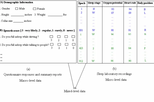
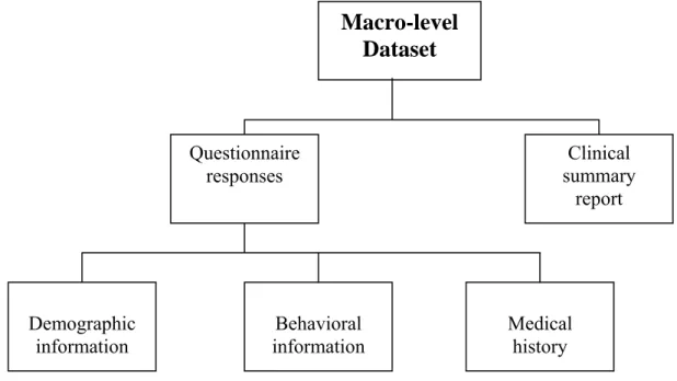
Fig. 4.1 Organization of data into macro, micro and mixed-level datasets
The questionnaire responses and summary reports providing overall statistics regarding pathological conditions, demographic and behavioral assessment of patients and clinical interpretations made by the physicians are combined together to form the macro-level dataset. Micro-level dataset includes epoch-by-epoch information of the patient’s sleep stages, oxygen potential, Electro-cardiogram readings of average heart rates every epoch, technician’s record of the patient’s body position during the epoch and recording of any
significant event of interest during the epoch. Mixed-level dataset is a compilation of all information used in macro and micro-level analysis. Only patients having both macro and micro-level information are considered while generating the mixed-level dataset. This dataset as a result has the least number of instances. In the remainder of this chapter we describe the data mining technique used to mine rules with relative time and evolution of a technique to mine rules with absolute time information over sleep data. In the chapters marked 5, 6 and 7 we describe in detail with experimental support how the technique has been used to perform macro, micro and mixed-level data analysis.
4.1 Association rule mining with time sequences
The sleep laboratory recordings collect data during every epoch of a patient’s sleep. In other words, the recordings are attribute-values measured at different times during the patient’s sleep. Hence, the data recorded for every patient during the entire night of sleep represents a time series. For mining association rules over time sequence attributes, the concept of events was introduced [Pra02]. Events are templates or patterns in data that capture time-related occurrences of interest. The temporal association rules are capable of representing all possible temporal relations that may be present among the set of events. In the domain of sleep analysis, a number of events can be identified depending on the objective of the analysis. For example, events of interest may include various stages in sleep or frequency of arousals that occur in a typical recording. The existing system captures the relationships between the events in relative time. For instance consider the following rule obtained from the rule-mining system.
sleepstage2 = 0:1 AND sleepstage2 = 4:5 Î sleepstageREM = 2:3
[Confidence = 79.49%; Support = 90.91%] This rule captures the temporal relationship between two events, viz., stage-2 of sleep and stage REM. The interpretation of the rule is as follows:
If a sleep stage-2 event is observed and later on another sleep stage-2 event is observed, then there is 79.49% likelihood that a REM stage event has occurred sometime in between the two stage-2 events. In other words, this rule with very high support and
confidence measures states that REM stage of sleep occurs in-between two occurrences of stage-2 of sleep. This is a well-known phenomenon of sleep progression known to sleep experts. The same rule can be represented diagrammatically in Figure 4.2. In this figure t0, t1, t2, t3, t4 and t5 represent arbitrary time indices that help sort the event
occurrences in time. Sleep stages REM stage-4 stage-3 stage-2 stage-1 Wake t0 t1 t2 t3 t4 t5 Relative Time
Fig. 4.2. Relative time variation of stage-2 and REM.
The extended association rule mining system helps understand the timing dependencies between the observed events. Thus, we obtain more information by mining over the time sequence variable than was possible using traditional association rule mining.
4.2 Event identification using filters
We wrote special filters to identify and isolate events of interest existing in the different datasets. For instance, sleep experts consider baseline oxygen potential to be an important marker or event. Baseline oxygen potential is the measurement recorded by the pulse oxymeter during the epoch when the person enters stage 1 of sleep with no event being observed for the first time since he/she drifted into sleep. Therefore, we wrote a special filter to identify and isolate epochs during the whole night sleep when the pulse oxymeter readings indicated values equal to or above baseline oxygen potential and
epochs during which the drops in oxygen potential measured more than three percent below the baseline potential. This process of converting the epoch-by-epoch data sequence into an event-based sequence leads to reduction in the size of the data. There are universally accepted ranges for deciding whether heart rates, oxygen potentials, body-mass index values are within normal or acceptable ranges. There are also additional ranges used in the field of medicine to identify the severity of the disorders if readings indicating the performance of the different physiological processes do not fall in the normal range. We wrote filters transforming the raw dataset to hold these range details.
4.3 Limitations in association rule mining with relative time
Mining of association rules with relative time information contained in them though sufficient to capture some interesting patterns in the sleep data does not uncover all the interesting patterns. For instance, just relative time is not sufficient when the time span between the events of interest or the length of time for which a particular event of interest was witnessed is considered important. Also in the domain of sleep analysis, the epoch periods in real-time during which certain events occurred or the length of time for which an event occurred is considered important since they can co-relate with pathology in many cases. They also help physicians to zero-in on a smaller subset of data or information to make their assessments. In order to address these limitations, we have extended the temporal association rules described above with time windows.
4.4 Temporal association rules using time windows
The WPI-WEKA system [Pra02] was designed to mine for rules over time sequences using relative time. To mine for rules with real-time information using the existing system we introduce the concept of windows. We divide the whole night sleep into equal-sized blocks called windows. Within these windows we identify the presence of different events of interest and the frequency with which the events occur within the windows.
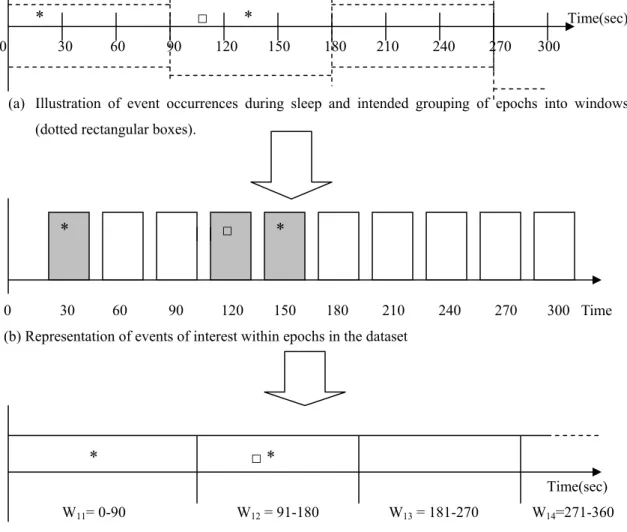
Figures 4.3 and 4.4 illustrate the aggregation of epochs into larger blocks of fixed size that we refer to as ‘windows’. Figure 4.3 shows a window formed by aggregating 3 contiguous epochs while figure 4.4 illustrates a window organized by aggregating 5 contiguous epochs together. Identical events may be noticed in contiguous epochs or they may recur with breaks or fragments (i.e., some epochs in-between may not have or experience the concerned event).
W12 W14
W11 W13
* □ * Time(sec) 0 30 60 90 120 150 180 210 240 270 300
(a) Illustration of event occurrences during sleep and intended grouping of epochs into windows (dotted rectangular boxes).
0 30 60 90 120 150 180 210 240 270 300 Time (b) Representation of events of interest within epochs in the dataset
* □ *
Time(sec)
W11= 0-90 W12 = 91-180 W13 = 181-270 W14=271-360
* □ *
(c) Grouping of epochs into windows and depicting of events noticed within them.
Fig. 4.3 Building windows from epochs (Window = 3 epochs = 90 seconds)
In figures 4.3 and 4.4, the * and □ represent events that occur during the patient’s sleep. The shaded areas in those figures represent the epochs when the events * and □ events are recorded.
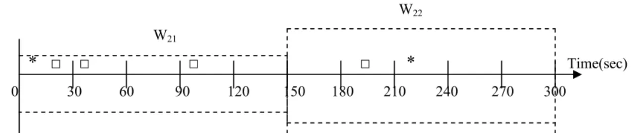
Another example of converting the dataset into one recording events of interest within windows is shown below.
W22
W21
* □ □ □ □ * Time(sec) 0 30 60 90 120 150 180 210 240 270 300
(a) Illustration of event occurrences during sleep and intended grouping of epochs into windows (dotted rectangular boxes).
0 30 60 90 120 150 180 210 240 270 300 Time (b) Representation of events of interest within epochs in the dataset
* □□ □ *
0-150 150-300 Time(sec) *
□ □ □
□ *
(c) Grouping of epochs into windows and depicting of events noticed within them.
Fig. 4.4. Building Windows from epochs (Window = 5 epochs = 150 seconds)
For simplicity in analyzing fragments detected within windows and to keep the input data format for our system simple, we make certain concessions. If the same event occurs during consecutive epochs within the same window, then they are represented as though a single event of the same type takes place within the window (no fragmentation witnessed). For instance, in Figure 4.4.b, we find that the event represented by symbol □ appears in two contiguous epochs (epoch 1 = 0-30 seconds and epoch 2 = 31-60
seconds). However, since it is the same event occurring in contiguous epochs (where all the contiguous epochs are contained within the same window), we consider only one occurrence of the event within the window. There is another □ symbol in the same window, which represents the fragmented event that occurs during epoch 4 (120 seconds). Hence Figure 4.4.c shows only 2 occurrences of □ event within the window. This process of crunching identical events occurring in contiguous epochs into one leads to the identification of the number of fragments of the particular event noticed within the window. This parameter is of medical significance. It becomes very interesting whenever we are able to detect multiple fragmentations of the same event within a single window.
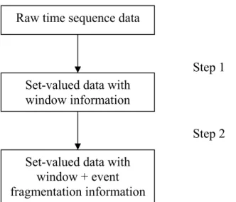
This technique is implemented in two steps with the help of the developed filters. The first stage involves the conversion of the sequence information in the raw dataset into a set-valued format. The set-values have the window-level information of the events that occur within them. The second stage is implemented by another filter, which accepts the transformed set-valued dataset as input to identify event-fragmentations within the windows. Pictorially the two-stage conversion process can be represented as shown in Figure 4.5.
Step 1 Raw time sequence data
Step 2 Set-valued data with
window information
Set-valued data with window + event fragmentation information
Fig. 4.5 Filters for transforming raw sequence data into set-valued with information on the windows within which events are witnessed along with the frequency of event-fragmentation
The difference in the representation of the events between the technique, which mines for rules with relative time information and our system which mines for rules in real-time can be explained with the help of Figure 4.4.b. In the figure we observe event □ occurs during the 1st, 2nd, 4th and 7th epochs of sleep. The system that mines rules in relative time would represent this event as a time sequence as follows.
Event □ = {1 : 2 ; 4 : 4 ; 7 : 7}1.
The same dataset after passing through the filters in our system will transform the events identified into a set-valued dataset as shown below.
Event □ = {event-□-0-150#2 ; event-□-150-300#1}
This is illustrated in Figure 4.4.c. Events occurring in epochs falling under a particular window are placed directly within that window. Thus, we are able to transform a time-series dataset with events into a set-valued dataset with the event information together with the frequency of the occurrence of the event within a window recorded. As can be clearly seen from the two representations, more information is obtained using our approach due to more detailed information. The size of the window is a user-specified value provided to the filters at the time of transformation.
We give an example of the nature of rules obtained using this technique below. stage-2 (750-800#1) && stage-R (750-800#1) && low-oxy (0-50#1) Î stage-W (300-350#1) && low-hrate (0-50#1)
[Confidence = 76.47%; Support = 10.74%; Lift = 2.1518; Chi-square = 14.4598; P<0.001] The rule states that when stage-2 and REM are noticed between the 750th to 800th epochs with low oxygen event in the first 50 epochs, wake state during the 300th and 350th epoch with low heart rate in the first 50 epochs of sleep is witnessed. The high chi-square value is indicative of the statistical robustness of the rule. The same rule can be diagrammatically represented as in Figure 4.6.
1 The actual input data file uses ‘^’ character instead of ‘;’ to separate epoch periods between which the
![Table 2.1: Simplified outline of the R&K sleep scoring criteria based on polysomnogram signals (Modified from Chapter 15, Page 1202, [CR94])](https://thumb-us.123doks.com/thumbv2/123dok_us/1726718.2742037/20.918.127.790.137.830/simplified-outline-scoring-criteria-polysomnogram-signals-modified-chapter.webp)