Logistics Research Centre
Assessment of the Opportunities for Rationalising
Road Freight Transport
Future Integrated Transport Programme
Link Research Project (FIT 022)
FINAL REPORT
Researchers:
Professor Alan McKinnon
Dr. Yongli Ge
Mr. David McClelland
Consortium Partners:
Cold Storage and Distribution Federation
Celsius First
Christian Salvesen
Isotrak
Master Foods
Optrak
February 2004
EXECUTIVE SUMMARY
This research project has contributed to the government’s objective of making freight distribution more sustainable in both economic and environmental terms. Its ‘Sustainable Distribution’ strategy aims to ‘ensure that the future development of the distribution industry does not compromise the future needs of our society, economy and environment’ (DETR, 1999). This can be partly achieved by getting companies to operate their lorries more efficiently by, among other things, reducing empty running, routing them more directly, increasing the vehicle load factors on laden trips and cutting energy consumption. A key element of the Sustainable Distribution strategy has been the Transport KPI initiative. The main aims of this initiative have been to: (i) enable companies to benchmark the efficiency of their road transport operations (ii) estimate average levels of efficiency at both sectoral and sub-sectoral levels and (iii) assess the potential for improving the efficiency of delivery operations.
To achieve these objectives it has been essential for participating companies to measure efficiency on a consistent basis. They have done this by collecting data over the same 48 hour period and recording it in specially constructed Excel workbooks. Synchronising the auditing process in this way has ensured that the fleets were exposed to similar trading conditions and road traffic levels during the survey period. The LRC developed the original transport KPI methodology and ran surveys for the DETR / DTLR / DfT in the food supply chain in 1997, 1998 and 2002. These contracts funded only a limited analysis of the survey data; calculating average KPI values at sectoral and sub-sectoral levels, preparing benchmark reports for participating companies and estimating potential reductions in cost, energy and emissions within several benchmark scenarios. This failed to exploit the full potential of the transport KPI data-base. In particular, no reference was made to the post-code data available for journey origins and destinations. It was recognised that analysis of this spatial data could permit an assessment of the potential for rationalising the distribution of food in the UK. In the previous transport KPI analysis this potential was assessed relative to current industry best practice. Geographical analysis of trip structure has made it possible to compare actual performance against theoretical optima under varying conditions.
The project has developed software tools which can be applied to a transport KPI database to assess the potential economic and environmental benefits of improving the efficiency of vehicle routing and exploiting backloading opportunities. The first set of tools interface the transport KPI data-base with the commercial vehicle routing package, Optrak. Individual trips are reconstructed and the route the vehicle actually followed compared with optimal routes that the vehicles could have followed under varying delivery time constraints. The second set assesses the potential for increasing the level of backloading. They extract relevant data from the Access data-base, reformat it, check it for consistency, geocode it and finally undertake a load matching analysis within various constraints. Additional geocoding software and several modules of the SAS package are used in the course of this analysis.
In recent years there has been a sharp increase in the number of trucks with onboard vehicle tracking systems. These tracking systems are being used primarily to provide transport managers with real time data on vehicle movements and thus improve day-to-day fleet management. Trips records are, nevertheless, being retained and permit detailed retrospective analysis of distribution operations. It was possible that, with further development, the software tools developed to conduct spatial analysis of the transport KPI data base might be adapted for use with these large commercial data-bases. In the later stages of the project, suppliers and users of road telematics systems were surveyed to determine the nature and scale of their data-bases, the extent to which they are currently being ‘data-mined’ and the demand from fleet managers for more detailed analysis of operational efficiency.
Transport KPI Survey Data
A total of 28 companies decided to participate in the 2002 survey, six of which committed more than one vehicle fleet, allowing them to undertake intra-company as well as inter-company benchmarking. The sample included four of the five largest supermarket chains in the UK. As the focus of the study was the load carrying unit, the activities of rigid vehicles and semi-trailers were surveyed, but not the tractor units of articulated trucks. The 3650 vehicles included in the survey travelled a total of approximately 1.45
million kilometres over the two-day period and delivered the equivalent of just under a quarter of a million pallet-loads. A total of 24,443 journey legs were monitored. Post-code data were provided for 12,364 (50.6%) of these legs. Many of the legs with post-code data, however, lacked a complete set of weight, pallet-load, distance and delivery time data. Comprehensive data were available for only 8995 legs. A broad cross-section of deliveries was monitored at three different levels in the food supply chain: primary (factory to regional distribution centre), secondary (regional distribution centre to supermarket or local wholesale depot) and tertiary (local distribution from wholesale depots to independent retailers and catering outlets). The survey also had national coverage, with sample fleets operating from bases well dispersed across the UK.
For the purposes of both the original benchmarking and the current analysis, fleets were divided into more homogeneous groups, mainly in relation to the level in the supply chain at which deliveries were made.
• Primary distribution between factories and RDCs (all articulated vehicles)
• Secondary distribution to supermarkets and superstores (mainly articulated vehicles) • Tertiary distribution to small shops and catering outlets (mainly rigid vehicles)
• Mixed distribution to large and small outlets (involving both articulated and rigid vehicles)
The analysis of routing efficiency was applied mainly to fleets involved in tertiary distribution. Their vehicles generally undertake multi-drop deliveries. The analysis of backloading potential, on the other hand, was confined to longer distance, single-drop deliveries at the primary and secondary levels.
Analysis of Routing Efficiency
Procedures were developed which (i) extract relative data from the transport KPI Access data base (ii) reconfigure it in an Excel spreadsheet (iii) input it into the Optrak vehicle routing package and (iv) perform calculations on the outputs of the Optrak modelling to estimate potential cost and emission reductions. At stages (ii) and (iii) in this process checks were made of the availability and validity of post-code data. The Optrak package requires postcodes with at least four digits. Across the fleets sampled, between 5 and 10% of delivery and collection points had missing or anomalous post-codes. As the delivery rounds analysed had an average of ten collection / delivery points, there was a high probability of a route having an inadequate set of post-code data. In an effort to maximise the sample of routes, considerable time was expended checking and, where possible correcting, post-codes. Within the available time it was only possible to check and analyse the routing data for a total of seven fleets. Over the 48 hour survey period they made a total of 469 trips for which adequate post-code data were available.
A comparison was made between the actual distances travelled and transit times, as recorded in the transport KPI survey, and the optimum values that could be achieved under varying conditions. Six scenarios were constructed in which three key scheduling variables were altered: length of the drivers’ shift, delivery time window at customers’ premises, opening and closing times at these premises. Scenario 1 (the ‘base’ scenario) used industry standard values typically adopted as defaults in routing packages. Detailed analysis of one company’s delivery operation, comprising the distribution of 744 food orders over two days in the south of England revealed that there was significant potential for reducing traffic, cost and emission, though the magnitude of the savings was very sensitive to scheduling constraints.
Analysis of Backloading Opportunities
A previous attempt by Cundill and Hull (1979) to analyse the potential for improving backloading in the UK was reviewed. This study had two major limitations. First, in the absence of information about the scheduling of trips and handling characteristics of the loads they had to over-simplify the load matching procedure and scale-down the number of ‘profitable matches’ by an arbitrary amount (75%). Second, their analysis was confined to freight movements to and from Swindon and Hull, which were not necessarily representative of the general pattern of road freight transport across the UK. The analysis of backloading potential using transport KPI survey data overcame these limitations.
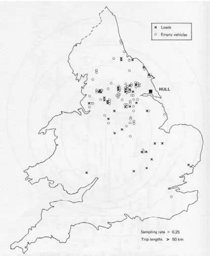
The first step in the backloading analysis involved finding empty journey legs that could potentially be allocated backloads. Initially the focus was on empty legs with a length of over 100 kilometres. A radius
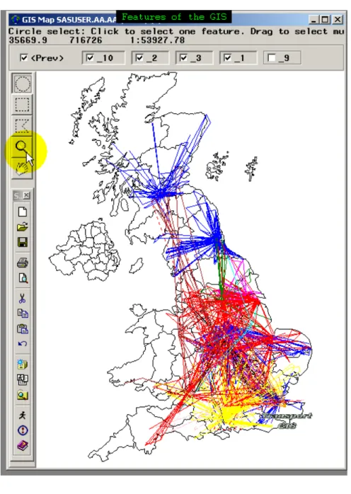
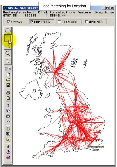
of 50 km around the origin and destination of the empty legs was then used to delimit a search zone for potential loads. Various levels of screening were applied to these potential loads relating to (a) location and direction of freight movement (b) vehicle compatibility (c) vehicle capacity and (d) delivery time window. The geographical information system (GIS) modules in the SAS package were used to store, manipulate, analyse and display this geographically-referenced data. Coding instructions were written in the SAS programming language to integrate spatial and attribute data and conduct the backloading analysis. An interactive query interface was established to enable the user to identify backloading opportunities on a company, zonal or individual trip basis. As distances were modelled on a ‘crow-fly’ basis, allowance had to be made for estuaries. This was done by routing journeys via strategically located ‘way-points’.
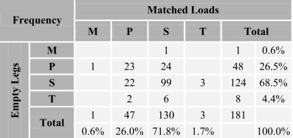
Of the 53 fleets (28 companies) which participated in the KPI survey, 29 fleets (13 companies) were selected for backloading analysis, those primarily engaged in longer distance trunking between factories, distribution centres and supermarkets. The final sample was composed of 2957 complete trips comprising 8995 legs with at least time and load information. Within this sample there were 573 empty journey legs longer than 100 kms. By matching the origins and destinations of loads it would have been possible to eliminate approximately a third of these legs (181). Each of these matches would save an average of 220 vehicle kms (after allowing for deviation from the direct return route). Across the sample of 13 companies, empty running would have been reduced by 13.7%. These backloading opportunities were analysed at sectoral, sub-sectoral and individual company levels. For example, sufficient data were provided by one major grocery retailer to assess the extent to which backloads could be generated internally within its transport system. Screening for vehicle compatibility (related mainly to temperature control), vehicle capacity (need to accommodate a backload in full) and scheduling (need for vehicle to return to base within two hours of the actual arrival time) reduced the number of load matches cumulatively by 48, 72 and 47. This meant that only 14 potential load matches met all four sets of backloading criteria, eliminating only 2.4% of all the empty legs longer than 100kms.
Limitations of the Transport KPI Survey Data
The transport KPI survey was designed to collect standardised vehicle operating data that could be used to benchmark the efficiency of companies’ road freight deliveries. As routing and backloading analysis was not in the original specification of the survey design, it is hardly surprising that the content and structure of the resulting data-set is not ideally suited to this type of research. If the DfT and its industry partners wish to make the analysis of routing and backloading an explicit objective of future transport KPI surveys it will be necessary to change this specification in several ways. The project reviewed the limitations of the transport KPI data and explained how they might be overcome. The main limitations were:
• Poor quality of much of the post-code data.
• Failure in the trip audit to differentiate drops and collections at an individual location.
• Failure to monitor the activities of the tractor unit: The transport KPI surveys in the food sector have focused attention on the load carrying unit (i.e. rigid vehicles and articulated trailers) This created a problem for the analysis of backloading potential because when assessing potential load matches it is important to know how tractors as well as trailers are scheduled.
• Lack of data on opening times, time-windows and driver shifts. In the absence of information about the actual opening times and delivery time windows at collection and delivery points and drivers’ hours, hypothetical values had to be used for the various scenarios. The modelling would be much more realistic if companies provided information about the degree of delivery flexibility.
• No differentiation of temperature-controlled vehicles in the trip audit: Inferences had to be made about the availability of refrigeration equipment from load data.
• Number of vehicles deployed on a particular delivery operation: this is not specified in the trip audit and therefore cannot be compared with the optimum numbers of vehicles determined by the Optrak package
• Insufficient density of trips: The effectiveness of the backloading analysis is critically dependent on the number of trips in the data-base. Despite the relatively high level of industry participation in the 2002 transport KPI survey and many thousands of journey legs surveyed, the number of potential load matches only supported detailed analysis at the first level of screening, related to the location of origins and destinations.
Surveys of Suppliers and Users of Vehicle Telematics Systems (VTS)
These surveys examined (i) the potential for vehicle telematics systems to collect operational data required for the calculation of transport KPIs (ii) the nature, formatting, storage and analysis of data currently collected (iii) the interfacing of road telematics databases with other software packages and (iv) the demand from vehicle operators for performance measurement systems. In the proposal it was suggested that telephone and face-to-face interviews would be supplemented by a ‘more extensive postal questionnaire survey’. A decision was made to drop the postal questionnaire survey and expand the telephone interview survey. Through personal contact with the companies, it was possible to obtain more information and discuss the technicalities of the service in greater detail. The success of this approach is reflected in the exceptionally high response rate for the survey of suppliers (33 companies: 89% response rate) and above-average response rate for the user survey (32 companies: 39% response rate). In-depth face-to-face interviews were held with four organisations. Questionnaires were designed and piloted for these surveys. Responses were coded and analysed using an Excel spreadsheet.
At present, telematic services are designed mainly to help companies improve time utilisation of vehicle assets, fuel efficiency and driver productivity. The current inability of VTS to monitor vehicle loading either directly through the use of sensors or indirectly through interfacing with other company IT systems is a major constraint on the wider of adoption of the vehicle utilisation measures promoted by the government’s transport KPI initiative. Indeed only one of the 33 telematics companies surveyed had the capability of monitoring all the variables required to measure the energy-intensity of a distribution operation. As load data is a key element in the spatial analysis of the transport KPI data, the applicability of the software tools developed by this project to commercial road telematics data-bases is currently limited. All the VTS suppliers surveyed provide retrospective analysis of tracking data, though the nature of this analysis and degree of customisation to client requirements varies widely. A third of the suppliers undertake benchmarking for clients, though in two-thirds of cases this is restricted to intra-company benchmarking. Only fifth of the sample of users claimed to use vehicle telematic data on a routine basis for calculating transport KPIs. There was, nevertheless, strong interest in making more use of this data for efficiency auditing and benchmarking. Three-quarters of the companies believed that more use could be made of tracking data to reduce empty running. The survey also detected disillusionment with this technology among some respondents who felt that several suppliers had ‘over-sold’ the systems and not provided enough guidance and after-sales support.
It was recognised at the outset that the commercial value of the tool-kit would be greatly enhanced if it could be deployed on a short-term basis to identify opportunities for improved loading. Following discussions with operators of road telematics systems and online freight exchanges, it has been concluded that the tool-kit lacks the functionality and is too closely customised to the transport KPI data to assume this role. Since the FIT proposal was originally prepared, several companies, such as Freight-traders, Teleroute and the Backload.com, have not only developed software capable of matching loads and available vehicle capacity but also created a transactional platform on which backhaul capacity can be traded. Their experience has shown that to provide a commercially viable load matching service it is necessary to handle a very high density trips. Their main problem has been generating the required volume of business rather than refining the software. As software for the real-time monitoring and trading of backhaul capacity has been now been developed and commercialised, with varying degrees of success, there seems little point in adapting our software tools for this purpose.
Deliverables
The main deliverable from this project has been the new set of software tools for retrospective analysis of the operational efficiency of truck fleets using data compiled in transport KPI-type surveys. They supplement the software which has already been developed by the LRC for the averaging and benchmarking of KPI values. Use of these tools permits the assessment of potential efficiency gains against theoretical optima, in contrast to the earlier benchmark analysis which judged this potential against prevailing industry best practice. It is anticipated that the main use of the tools will be to estimate potential cost, energy and emissions savings at an aggregate level, though they could be applied to a single company’s transport operation where it supplies sufficient fleet data. The transferability of the tools will be partly constrained by their integration with the Optrak and SAS software packages and by the degree of
customisation to the existing transport KPI methodology. Other deliverables include (i) the results of the routing and backloading analyses on which the new software tools were tested and (ii) the results of the surveys of companies supplying and using road telematics systems. The latter results provide a useful insight into the current state of the telematics sector in the UK and the possibility of applying a similar set of software tools to commercial vehicle tracking data bases.
CONTENTS
SECTION 1. INTRODUCTION ... 9
1.1 TRANSPORT KPIINITIATIVE: ... 9
1.2 SPATIAL ANALYSIS OF TRANSPORT KPIDATA... 10
1.3 ANALYSIS OF ROAD TELEMATICS DATA... 11
1.4 OBJECTIVES OF THE PROJECT... 12
1.5 STRUCTURE OF THE REPORT... 12
SECTION 2. THE TRANSPORT KPI DATA-BASE... 14
2.1 CHOICE OF KPIS... 14
2.2 SAMPLE OF COMPANIES,FLEETS AND VEHICLES... 16
2.3 METHOD OF DATA COLLECTION... 20
2.4 CLASSIFICATION OF THE FLEETS... 22
SECTION 3. OPTIMISATION OF VEHICLE ROUTING... 24
3.1 METHODOLOGY... 24
3.2 FLEET SELECTION... 25
3.3 DATA INPUT INTO THE OPTRAK MODEL... 26
3.4 KEY FACTORS CONSIDERED... 27
3.4.1 key parameters for the base scenario ... 27
3.5 SCENARIO ANALYSIS... 28
3.5.1 Major outputs ... 28
3.5.2 Results of the Routing Analysis ... 31
3.5.3 Benefits of More Efficient Vehicle Routing ... 36
SECTION 4. BACKLOADING ANALYSIS ... 38
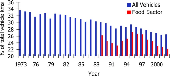
4.1 EMPTY RUNNING TREND IN THE UK ... 38
4.1.1 Empty Running in the Food Supply Chain ... 44
4.2 METHODOLOGY USED IN THE PRESENT STUDY... 48
4.3 FLEET SELECTION... 50
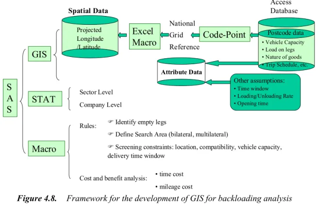
4.4 GIS DEVELOPED FOR BACKLOADING ANALYSIS... 50
4.4.1 Features of the Food Transport GIS ... 51
4.4.2 Screening of Potential Backloads... 52
4.5 BACKLOADING ANALYSIS... 54
4.5.1 Location Screening... 54
4.5.2 Vehicle compatibility screening ... 59
4.5.3 Vehicle capacity screening ... 60
4.5.4 Time screening ... 60
4.6 POTENTIAL SAVINGS... 60
SECTION 5. LIMITATIONS OF THE TRANSPORT KPI SURVEY DATA ... 62
5.1 QUALITY OF THE POST-CODE DATA... 62
5.2 DIFFERENTIATION OF DROPS AND COLLECTIONS... 63
5.3 MONITORING OF TRACTOR USAGE... 63
5.4 OPENING TIMES,TIME-WINDOWS AND DRIVER SHIFTS... 64
5.5 DIFFERENTIATION OF TEMPERATURE-CONTROLLED VEHICLES... 64
5.6 NUMBER OF VEHICLES DEPLOYED ON A PARTICULAR DELIVERY OPERATION... 65
5.7 INSUFFICIENT DENSITY OF TRIPS... 65
SECTION 6. ASSESSING THE POTENTIAL FOR VEHICLE TELEMATICS SYSTEMS TO PRODUCE KEY PERFORMANCE INDICATORS ... 67
6.1 INTRODUCTION... 67
6.2 METHODOLOGY... 68
6.2.1 Population and Sample ... 68
6.2.2 Questionnaire ... 69
6.2.3 Questionnaire ... 70
6.2.4 Collection of Data Sections 1 & 2... 70
6.3.1 1. Suppliers of Vehicle Telematics Systems ... 71
6.3.2 Users of Vehicle Tracking Suppliers ... 83
6.4 CONCLUSION... 92
SECTION 7. ACHIEVEMENT OF OBJECTIVES... 93
SECTION 8. DELIVERABLES... 98
SECTION 9. DISSEMINATION ... 99
SECTION 10 MANAGEMENT OF THE PROJECT ... 101
SECTION 11 GLOSSARY... 102
SECTION 12 APPENDICES ... 106
Acknowledgement
We wish thank all the organisations which have which have contributed to this project. We are particularly grateful to the industrial partners for their support and encouragement throughout. The Cold Storage and Distribution Federation deserve special mention as they have worked closely with the Logistics Research Centre over the past seven years on the transport KPI initiative which has formed the basis of the present project. We are also very grateful to the Department for Transport for funding this project as part of the joint DfT / EPSRC Future Integrated Transport programme. Finally, our thanks also go the numerous suppliers and users of vehicle tracking systems which participated in the interview survey.
Contact Details Logistics Research Centre
Heriot Watt University EDINBURGH UK EH14 4AS Tel 0131 451 3850 Fax 0131 451 3498 Website: http//www.sml..hw.ac.uk/logistics
SECTION 1. INTRODUCTION
1.1 TRANSPORT KPIINITIATIVE:
This research project has contributed to the government’s objective of making freight distribution more sustainable in both economic and environmental terms. Its ‘Sustainable Distribution’ strategy aims to ‘ensure that the future development of the distribution industry
does not compromise the future needs of our society, economy and environment’ (DETR,
1999). This can be partly achieved by getting companies to operate their road freight vehicles more efficiently by, among other things, reducing empty running, routing vehicles more directly, increasing the vehicle load factors on laden trips and cutting energy consumption. A key element of the Sustainable Distribution strategy has been the Transport KPI initiative. This was instigated in 1997 by several companies belonging to the Cold Storage and Distribution Federation (CSDF) which were concerned about the downward pressure on vehicle load factors at a time when road transport costs were rising. They were keen to explore ways in which they could work together to improve vehicle utilisation. The government provided financial support for the initiative under its Energy Efficiency Best Practice Programme (EEBPP) (now renamed the TransportEnergy Best Practice Programme), recognising that if it was successful it could yield significant savings in fuel and CO2 emissions and reductions in lorry traffic levels.
The main aims of the transport KPI iniative have been to:
• enable companies to benchmark the efficiency of their road transport operations
• estimate average levels of efficiency at both sectoral and sub-sectoral levels
• assess the potential for improving the efficiency of delivery operations
To achieve these objectives it has been essential for participating companies to measure efficiency on a consistent basis. They have done this by collecting data over the same 48 hour period and recording it in specially constructed Excel workbooks. Synchronising the auditing process in this way has ensured that the fleets were exposed to similar trading conditions and road traffic levels during the survey period.
To date, six transport KPI surveys have been undertaken in four sectors, and one is currently underway (Table 1.1). This research project has been based on the results of the survey
conducted in the food supply chain in May and October 20021. This survey employed a methodology originally developed by the Logistics Research Centre in 1997 and subsequently refined. The LRC’s contracts to run the 1997, 1998 and 2002 transport KPI surveys in the food sector funded only a limited analysis of the survey data. This involved calculating average KPI values at sectoral and sub-sectoral levels, preparing benchmark reports for participating companies and estimating potential reductions in cost, energy and emissions within several benchmark scenarios (McKinnon, 1999; McKinnon, Ge and Leuchars, 2003a and 2003b, Energy Efficiency Best Practice Programme, 1998 and 1999).
Table 1. 1 . Transport KPI Surveys
Sector Survey Date
Temperature-controlled food 1997
Food (all temperatures) 1998
Automotive 2001
Food (all temperatures) 2002
Non-food retailing 2002
Road leg of air cargo distribution 2002-3
Pallet-load networks 2004
1.2 SPATIAL ANALYSIS OF TRANSPORT KPIDATA
The earlier analysis failed to exploit the full potential of the transport KPI data-base. In particular, no reference was made to the post-code data available for journey origins and destinations. It was recognised that analysis of this spatial data could permit an assessment of the potential for rationalising the distribution of food in the UK. In the previous transport KPI analysis this potential was assessed relative to current industry best practice. Geographical analysis of trip structure has made it possible to compare actual performance against theoretical optima under varying conditions. The original intention was to assess the potential economic and environmental benefits of rationalising road freight operations in four ways:
• Increasing the backloading of returning delivery vehicles
• Improving the routing of vehicles
• Rescheduling deliveries
• Increasing the degree of load consolidation
1 In the original proposal it was indicated that data from the 1998 KPI survey would be analysed. By the time the project actually started in December 2002, this survey had been updated and expanded.
The first two measures have been analysed in detail. The effects of the third measure, delivery rescheduling, have been modelled in relation to vehicle routing options. The sensitivity of journey length, cost and transit time to variations in opening times and delivery time windows have been assessed. It has proved impractical, however, to estimate the opportunities for consolidating loads moving between proximate origins and destinations. Given the variability of load weights and dimensions, temperature-control requirements, vehicle handling systems and scheduling, it is extremely difficult to determine the probability of achieving an acceptable match between two or more partial loads on particular corridors. The research has therefore been confined to the first three rationalisation measures.
To conduct this analysis it has been necessary to develop new software tools. The first set of tools interface the transport KPI data-base with the commercial vehicle routing package, Optrak. These tools require a significant amount of manual input. Individual trips are reconstructed and the route the vehicle actually followed compared with optimal routes that the vehicles would have followed under varying delivery time constraints. The second tool set assesses the potential for increasing the level of backloading. These tools extract relevant data from the Access data-base, reformat it, check it for consistency, geocode it and finally undertake a load matching analysis within various constraints. Additional geocoding software and several modules of the SAS package are used in the course of this analysis.
1.3 ANALYSIS OF ROAD TELEMATICS DATA
In recent years there has been a steep increase in the number of trucks with onboard vehicle tracking systems. These tracking systems are being used primarily to provide transport managers with real time data on vehicle movements and thus improve day-to-day fleet management. Trip records are, nevertheless, being retained and permit detailed retrospective analysis of distribution operations. It was possible that, with further development, the software tools developed to conduct spatial analysis of the transport KPI data base might be adapted for use with these large commercial data-bases. In the later stages of the project, suppliers and users of road telematics systems were surveyed to determine the nature and scale of their data-bases, the extent to which they are currently being ‘data-mined’ and the demand from fleet managers for more detailed analysis of operational efficiency. While the general analytical procedures developed in this project will be applicable to commercial road telematics
data-bases, the actual tools have had to be so closely customised to particular aspects of the transport KPI database that they are unlikely to be directly transferable.
1.4 OBJECTIVES OF THE PROJECT The project had six objectives:
• To define and specify the requirements for the software tool-kit
• To develop a software tool-kit for use on the 2002 transport KPI database for the food sector
• To apply the tool-kit in an analysis of this database to assess the potential for reducing the economic and environmental costs of road freight transport
• To consider how the tool-kit might have to be adapted to distribution operations in other sectors • To examine the collection of KPI data by commercial road telematics systems
• To investigate ways of combining the software tool-kit with real-time road freight information systems to identify backloading and load consolidation opportunities on a short-term basis.
Figure 1.1 shows how the research project was organised to achieve these objectives. Details of the management of the project can found in Section 10.
1.5 STRUCTURE OF THE REPORT
The remainder of the report is divided into nine sections:
Section 2 outlines the nature and extent of the 2002 food transport KPI database, the consistency checks that have been undertaken and the classification of fleets into sub-sectors. Section 3 focuses on the efficiency of vehicle routing. It describes the software developments required to interface the transport KPI database with the Optrak vehicle routing package. The results of the analysis of routing efficiency within varying time constraints are then reported. Section 4 examines the potential for improving backloading. Previous research on the empty running and backloading of trucks is reviewed. The development of software tools for this part of the analysis is then outlined. Backloading opportunities are assessed at four levels of load-matching.
Section 5 considers the limitations of the transport KPI database for this type of spatial analysis and recommends changes to the methods of data collection and management that would facilitate future modelling of potential efficiency gains.
Section 6 reports the results of two surveys of suppliers and users of vehicle tracking systems. These enquired about the nature of the telematics services, the use currently being made of the
transport databases, the software interfaces and future plans for the use of tracking data for KPI measurement.
Section 7 assesses the extent to which the original objectives of the project have been achieved against technical, commercial, financial and other criteria.
Section 8 outlines the main deliverables of the project.
Section 9 addresses the issue of dissemination. It lists papers already prepared and plans for future publications and conference papers.
Section 10 provides details of the management of the project. Section 11 contains a glossary of terms.
Section 12 comprises seven appendices on various aspects of the project.
Figure I. 1 .Structure of the Research Project
Familiarisation with transport KPI method, software and database
Checking and inputting KPI data for fleets surveyed in October 2002
Modification to KPI Access database to facilitate data handling
Training in the use of the Optrak
routing package
Development of software tools for routing analysis
Checking, validating, correcting post-code
data
Analysis of routing efficiency under varying
scheduling constraints
Development of software tools for
routing analysis
Development of an analytical framework for
backloading analysis
Self-training in the use of the SAS software package
Geo-coding and correction for routing
around ‘way points’
Analysis of backloading opportunities at different levels
of load-match screening
Review of deficiencies in the transport KPI survey method and database
Recommendation of improvements to the transport KPI survey method
Review of the market for vehicle telematics systems
(VTS) in the UK Review of empty running
trends and previous research on backloading
Design of survey of VTS suppliers and users: preparation of questionnaires
Compiling sampling frames of suppliers and users of VTS
Telephone / face-to-face interview surveys
Coding and analysis of VTS survey results Preparation of Final Report
SECTION 2. THE TRANSPORT KPI DATA-BASE
2.1 CHOICE OF KPIS
The use of KPIs to monitor the efficiency and effectiveness of logistics has been discussed by the Nevem Workgroup(1989), Caplice and Sheffi (1994 and 1995), Ploos van Amstel and D’hert (1996) and van Donselaar and Sharman (1998). Long lists of possible KPIs have been compiled to assess the performance of many different aspects of a logistical operation. Inter-company benchmarking of logistical KPIs is also well established (Hanman, 1997; Randall, 2003).
The original selection of KPIs for this initiative back in 1997 was restricted in several respects. First, it related solely to the transport function. Second, it excluded any reference to the cost of transport operations. Initial consultations with CSDF members revealed that few companies would be prepared to divulge this information. The KPIs were designed therefore to measure operational, rather than commercial, performance. It has, nevertheless, been possible to convert some of the performance measures into cost estimates using industry standard cost data, such as that published in the Motor Transport Cost Tables. Third, unlike many performance measurement systems which are internal to a single business and thus tailored to its requirements, the KPIs adopted for this project had to win acceptance from firms across an business sector. They had also to relate to the wider impact of transport operations on the environment in contrast to many of the traditional metrics which are concerned solely with economic efficiency (McIntyre et al.,1998).
Caplice and Sheffi (1994) have differentiated three types of logistics KPI:
Utilisation indices which measure ‘input usage’ and are usually expressed as a ratio of the actual input of resources to some normative value.
Productivity indices which measure ‘transformational efficiency’ and typically take the form of input : output ratios.
Effectiveness indices which measure the ‘quality of process output’ as a ratio of the actual quality achieved to some norm.
The vehicle audit employed all three types of KPIs, ensuring that the assessment was broadly-based and concerned with both inputs and outputs.
Discussions were held with senior managers of manufacturing, retailing and logistics firms to canvas their opinions on possible KPIs. At a ‘think tank’ session they debated the various options and examined the practical problems they might pose. The derivation of the KPIs was, therefore, a ‘bottom-up’ exercise involving close consultation with industry. The KPIs had to meet several requirements. They had to be:
• defined in clear and unambiguous terms so that they could be easily understood by staff responsible for data collection
• capable of direct and detailed measurement at operational level
• measurable in a consistent manner by all participating companies
• compatible with data recording systems already in place and software packages with which company staff were familiar
• correlated with operating costs and energy consumption
• of direct relevance to the management of the transport operation
• widely acceptable across the industry and of possible application in other sectors.
The deliberations with senior managers led to the establishment of an agreed set of five KPIs. The first three KPIs were essentially ‘utilisation’ measures, the fourth was a ‘productivity’ index and the last assessed the ‘effectiveness’ of the delivery operation:
1. Vehicle loading: this was measured by ratio of the actual load carried to the maximum load that could have been carried within with vehicle weight, floorspace and height constraints. 2. Empty running: the distance the vehicle travelled empty (excluding the return movement of
empty handling equipment, which was separately recorded).
3. Fuel consumption: for both motive power and refrigeration equipment.
The fuel efficiency of the tractor units was expressed on a km-per-litre basis and averaged across the fleet on an annual basis. No attempt was made to estimate fuel consumption during the 48 hour survey period as this was considered impractical. These estimates would, after all, relate to tractor units, whereas the main survey unit was the trailer. The same tractor might haul several different trailers during the survey period. Annual average litres / km figures were obtained for each type of vehicle within each fleet. These were multiplied by the distances travelled during the survey period to obtain estimates of fuel consumption.
The first three KPIs were used to develop a composite measure of energy-intensity. As food is a relatively low density product, loads moved by truck tend to be volume-constrained rather than weight-constrained. It was decided, therefore, to express energy-intensity in terms to pallet-kilometres rather than tonne-kilometres. It was defined as the amount of fuel required to move one pallet one kilometre (excluding fuel consumed by the refrigeration equipment.)
4. Vehicle time utilisation: This was measured at hourly intervals over a period for 48 hours for all the trailers surveyed. A record was made of the dominant activity of the trailer over the previous hour. Time was classified into seven activities depending on whether the vehicle was: running on the road, being loaded / unloaded, pre-loaded awaiting departure, awaiting loading / unloading, undergoing maintenance / repair, in driver daily rest period or idle (i.e. empty and stationary).
5. Deviations from schedule: This KPI was included because instability in transport schedules can have a bearing on vehicle utilisation as it makes it more difficult for companies to plan backhauls and more complex multiple collection / delivery rounds. Companies were asked to specify the main cause of any delay as being: a problem at collection point (responsibility of the consigning company), a problem at delivery point (receiving company’s responsibility), the actions of the company undertaking the delivery (‘own company action’), traffic congestion, equipment breakdown or the lack of a driver.
Only data collected for the calculation of the first three KPIs, relating to vehicle fill, empty running and fuel consumption, was used in the present project. The time utilisation data was collected on a separate spreadsheet and was not trip-related. Information on deviations from schedule was trip-related and could have been incorporated into the routing and backloading analysis either for specific trips or as a generalised probability function. Within the project time-frame this has not been possible. Future development of the modelling will try to make allowance for unreliability in the food distribution system.
2.2 SAMPLE OF COMPANIES,FLEETS AND VEHICLES
A questionnaire survey of companies participating in the 1998 audit revealed that on average approximately five days of staff time were required per fleet to set up and implement the internal data collection procedures. This was in addition to the time that company representatives spent attending briefing sessions. As participation in the survey required
companies to make a significant resource commitment, the initiative had to be intensively marketed. Promotional activities were organised by the CSDF. A conference, press articles, telephone calls and company visits were used to publicise the survey.
A total of 28 companies decided to participate in the 2002 survey, seven of which committed more than one vehicle fleet, allowing them to undertake intra-company as well as inter-company benchmarking. The sample included four of the five largest supermarket chains in the UK. As the focus of the study was the load carrying unit, the activities of rigid vehicles and semi-trailers were surveyed, but not the tractor units of articulated trucks. The 3650 vehicles included in the survey travelled a total of approximately 1.45 million kilometres over the two-day period and delivered the equivalent of just under a quarter of a million pallet-loads (Table 2.1). The survey monitored just over 13 million tonne-kms of freight movement in the grocery sector over the two-day period.
A total of 24,443 journey legs were monitored. Post-code data were provided for 12,364 (50.6%) of these legs. Table 2.1 shows the proportion of post-codes with varying numbers of digits. Many of the legs with post-code data, however, lacked a complete set of weight, pallet-load, distance and delivery time data. Comprehensive data were available for only 8995 legs. Tables 2.2 and 2.3 shows the distance and transit time profiles for the full sample of journey legs. In the backloading analysis, a distance of 100km was adopted as the minimum leg length required for viable load matching.
Table 2. 1 . Availability of post-code data
Total journey legs 24,443 100%
Legs with some post-code data 12,364 50.6%
Legs with full post-code 10,040 41.1%
Legs with 5-digit post-code 1,662 6.8%
Legs with 4-digit post-code 591 2.4%
Table 2. 2 . Distribution of Journey Legs by Length
Distance (km) Number of legs
Table 2. 3 . Distribution of Journey Legs by Duration
<10 6,163 >10 17,760 >20 15,144 >30 13,245 >40 11,479 >50 9,957 >60 8,706 >70 7,566 >80 6,543 >90 5,703 >100 5,050 >150 2,558 >200 1,183 >250 509 >300 178 < 00:30 9,737 > 00:30 12,668 > 01:00 8,970 > 01:30 6,290 > 02:00 4,360 > 02:30 3,010 > 03:00 1,997 > 03:30 1,228 > 04:00 838 > 04:30 504 > 05:00 303 > 05:30 178 > 06:00 100
Duration (hour) Number of legs
A broad cross-section of deliveries was monitored at three different levels in the food supply chain: primary (factory to regional distribution centre), secondary (regional distribution centre
to supermarket or local wholesale depot) and tertiary (local distribution from wholesale depots to independent retailers and catering outlets) (Figure 2.1).
Production
Primary Consolidation Centre
Independent retail
outlet catering outlet Multiple retail outlet Local wholesale / cash and carry
warehouse Regional Distribution Centre
(supermarket chain)
Regional Distribution Centre (large wholesaler) Secondary
Primary
Tertiary
Figure 2.1. Distribution Channels in the Food Sector
The survey also had national coverage with sample fleets operating from bases well dispersed across the UK (Figure 2.2).
Table 2. 4 . Comparison of Key Survey Parameters
Transport KPI
Survey
CSRGT1
‘other foodstuffs’ category
Full loading % by weight 13% 11%
Full loading % by volume 37% 31%
% empty running 19% 22%
Average vehicle lading factor 53% 56%
Average fuel efficiency: (km per litre) all road freight operations
Small rigid (2 axles) < 7.5 tonnes 4.0 4.1
Medium rigid (2 axles) 7.5 - 18 tonnes 3.6 3.7 (7.5-14t) - 3.3 (14 -17t) Large rigid (> 2 axles) > 18 tonnes 3.1 2.9 (17-25t) 32 tonne articulated vehicle (4 axles) 3.2 3.2 (< 33t) 38-44 tonne articulated vehicle (>4 axles) 2.9 2.9 (> 33t)
1. Continuing Survey of Road Goods Transport
The sample of companies and fleets was not the result of random selection. Care must therefore be exercised in interpreting the aggregate results as these may not be representative of the food supply chain as a whole. An indication of the representativeness of the sample can, nevertheless, be obtained by comparing some of the survey results with corresponding values
from the government’s Continuing Survey of Road Goods Transport (CSRGT), which is based on a much larger, randomly-generated sample of vehicles. The average values for some of the key parameters are similar (Table 2.4), suggesting that the road transport operations monitored over the two-day period are fairly representative of the general movement of food by road in the UK2.
Figure 2.2. Locations of the Main Bases of the Sample Fleets
2.3 METHOD OF DATA COLLECTION
Having committed themselves to the survey, companies were asked to assign appropriate staff to the collection and collation of transport data (Figure 2.3). They were invited to three briefing sessions run by the CSDF and LRC at which the data collection process was outlined in detail. Definitions were clarified and advice given on the methods of collecting and recording the information. At these sessions, companies were issued with manuals and CDs containing the standard Excel workbook into which the data was to be entered. It was then the responsibility of companies to decide on the numbers, types and locations of vehicles to be surveyed. Some identified a sample of vehicles at a particular location, while others committed
whole fleets based at one or more depots. Transport and logistics managers had also to work out how to manage the data collection process internally. This usually involved the delegation of tasks to supervisors, clerks and drivers and liaison with IT staff.
Company commitment to participate Assign appropriate staff
Attend briefing session Make internal arrangements: - select vehicles to survey - staff briefing
- operations / IT liaison
Internal calculation of KPIs COLLECT DATA Transfer raw data
to LRC
Check for data consistency Liaision with companies to rectify
anomalies Analysis:- pooling of data - aggregate values - benchmarking Distribution of benchmark data Preparation of reports
Figure 2.3. Process of Collecting Transport KPI Data
Participating companies were asked to enter their operating data into a standard Excel workbook comprising three spreadsheets for:
1. General data on the vehicle fleet
2. Data on all trips performed during the 48 hour period 3. Hourly audit of vehicle activity during this period. Appendix A contains copies of these spreadsheets.
Once the data was collected companies were able to calculate their KPI values themselves using macros embedded in the Excel workbook. The spreadsheets containing the ‘raw data’ were then returned to the LRC for checking, aggregation and analysis.
Consistency checks were made both at the time of data entry and prior to analysis. The initial check ensured that data fell within acceptable ranges. Once all the data was entered, higher-level checks detected anomalies and missing values. Where these would have significantly affected the analysis the company was contacted in an effort to correct/complete their data-set.
All participating companies were sent benchmark reports for each of their fleets in which their operation efficiency was compared with sectoral and sub-sectoral averages.
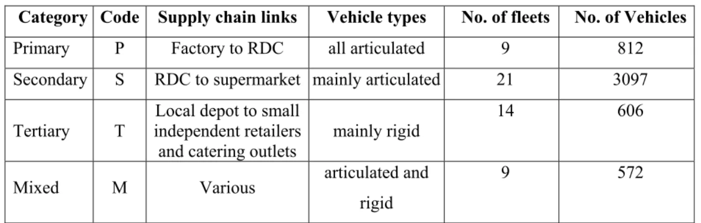
2.4 CLASSIFICATION OF THE FLEETS
The sample contained fleets engaged in a diverse range of distribution operations. To improve the validity of the benchmarking it was necessary to split the fleets into more homogeneous groups, mainly in relation to the level in the supply chain at which deliveries were made.
• Primary distribution between factories and RDCs (all articulated vehicles) (P)
• Secondary distribution to supermarkets and superstores (mainly articulated vehicles) (S)
• Tertiary distribution to small independent shops and catering outlets (mainly rigid vehicles) (T)
• Mixed distribution to large and small outlets (involving both articulated and rigid vehicles) (M)
Table 2. 5 . Classification of Sample Fleets and Vehicles by Sub-Sector
Category Code Supply chain links Vehicle types No. of fleets No. of Vehicles
Primary P Factory to RDC all articulated 9 812
Secondary S RDC to supermarket mainly articulated 21 3097
Tertiary T
Local depot to small independent retailers
and catering outlets mainly rigid
14 606
Mixed M Various articulated and
rigid
9 572
Table 2.5 shows the number of fleets in each category. The fourth category contained mixed fleets engaged in different types of delivery operation. The average KPI values for these mixed fleets partly depend on the balance between trunking and local delivery activities.
The analysis of routing efficiency was applied mainly to fleets involved in tertiary distribution. Their vehicles generally undertake multi-drop deliveries. The sequencing of drops within the delivery rounds is the main determinant of routing efficiency. Most of the road freight movements at the primary and secondary levels of the supply chain are single drop deliveries. The analysis of backloading potential, on the other hand, was confined to longer distance, single-drop deliveries at the primary and secondary levels. Backloading is generally only economical on longer journey legs (except where the return load can be picked up the delivery
point). Furthermore, on multiple-drop rounds empty running is usually confined to the last leg of the journey back to the depot, which is typically fairly short.
SECTION 3. OPTIMISATION OF VEHICLE ROUTING
3.1 METHODOLOGY
The potential for improving the efficiency of fleet operation will be examined by interfacing commercial vehicle routing and scheduling software package Optrak with the KPI 2002 survey in the food sector. Optrak is a computer system which plans efficient vehicle loads and routes. It combines road network data with information on vehicles, customers, orders, depot location and timing to produce a set of trips that makes the best use of available resources.
The main objectives of interfacing Optrak with the KPI 2002 survey database are to see (a) to what extent to routing of vehicles monitored in the 2002 transport KPI survey is sub-optimal and (b) the sensitivity of delivery efficiency to variations in service parameters.
Fleet selection
Only fleets heavily involved in multiple-drop delivery were included in this analysis. These mostly belonged to the tertiary and mixed categories. Fleet selection also took account of the quality of the spatial data provided by the company. As explained in greater detail in Section 5, much of the post-code data was inaccurate. Given the large amount of time required to check the validity of post-codes and eliminate trips containing inaccurate post-code data, priority was given to those fleets which, on the basis of sampling, appeared to have the most accurate post codes. Within the time allocated for this part of the project, the routing efficiency of seven fleets representing was analysed. A range of different distribution systems were selected for this optimization analysis. It included a group of fleets from the same company in the same sector, a group of fleets from the same company but different sub-sector, and a group of fleets within the same sub-sector, but from different companies.
Data preparation
The relevant information in the KPI 2002 survey database was converted into different CSV (Comma Separated Values) files required by Optrak as follows:
) customer.csv ) depot.csv ) driver.csv ) opentime.csv ) order.csv ) product.csv ) vehicle.csv
The required data was extracted from the Access database and stored in separate CSV files in Excel spreadsheets. Within Excel they were formatted for input into Optrak .
Scenario analysis
Seven delivery scenarios were constructed to assess the degree of routing efficiency for a sample of fleets under different operating conditions. These conditions were defined with respect to driver shifts, opening times and delivery time windows.
3.2 FLEET SELECTION
The following three groups of fleets were selected for optimisation using Optrak:
) Same company, same sub-sector (Tertiary Distribution)
The first group of fleets were all within the same company and the same sub-sector. This included two fleets involved in tertiary distribution. A total of 96 valid trips and 847 journey legs (including empty legs) were selected.
) Same company, different sub-sector
The second group of fleets were all within the same company but each from different sub-sector (which involves secondary, tertiary, and mixed distribution). This group was composed of three fleets, with a total of 338 valid trips and 1129 journey legs selected.
) Same sub-sector, different company (Primary temperature controlled distribution)
The third group of fleets was composed of two fleets within the same sub-sector (primary temperature controlled distribution) but from different company. A total of 35 valid trips and 98 journey legs were selected.
3.3 DATA INPUT INTO THE OPTRAK MODEL Customer data
Optrak defines a customer as a delivery/collection location. Each delivery address needs a unique code. Optrak can use grid reference, postal code, or town name to determine a customer’s location. In the models developed for this project, customer locations were determined using postcodes stored in the KPI database.
Orders
An order record contains the order details, such as its reference number, the customer involved, whether it is a delivery or a collection, how much of which product is to be carried and which visiting times apply. This is the header record consisting of general information about an order. The detailed information of each additional part of an order is held in the order parts file that is linked to the orders file.
Drivers
The time drivers spend working and driving is restricted by legislation and labour agreements. The planning of trips takes account of driver availability and no schedule will be produced which infringes regulations controlling driver hours. Driver’s work regulations and other constraints include shift length, shift driving, shift work, shift gap, break length, break after driving, breaking after working, etc. Besides, individual driver’s preference of working time can be specified in a separate form.
Vehicles
The vehicles file describes the number of vehicles that can be used in the trip schedules, which depot(s) a vehicle belongs to, the maximum weight/volume that can be carried on the vehicle, and cost of operation including distance-related and time-related cost elements. The vehicle cost information is obtained from Motor Transport’s vehicle cost tables (Anon, 2002).
Load/unload rates
These loading and unloading rates model the loading/unloading process. Loading and unloading times can have a large impact on the quality of routes, especially if loading and unloading take up a large proportion of the working day.
Opening times
Each customer and depot must have a record which specifies opening times on a daily and weekly basis. This allows the optimisation algorithms to schedule trips so that a vehicle arrives at a customer in good time for all loading and unloading to be completed before closing time. Depots
The depots file contains general information on the depot(s), its location, opening times, vehicle restrictions and load rates.
3.4 KEY FACTORS CONSIDERED
The following key factors included in this optimisation exercise: driving hours, customer demand time window, customer/depot opening time, loading/unloading rate.
3.4.1key parameters for the base scenario 3.4.1key parameters for the base scenario
The base scenario (scenario 1) is established using parameters used in common practice.
Shift length: maximum duration of a shift (11:00) including driving loading/unloading, and break(s).
Shift driving: maximum total driving time in a shift (9:00).
Shift gap: minimum time between the end of one shift and the start of the next (13:00). Break length: minimum length of a break (0:45).
Break after driving: maximum driving time without taking a break (4:30). Break after working: maximum working time without taking a break (5:30). Loading/unloading rate: depot (0:30), customer sites (3 minutes/pallet).
(Consultation with industry patterns indicated that the ratio of loading / unloading time for wooden pallets and roll cages was 4:1. Typically a roll cage would be offloaded in 70 seconds, a wooden pallet in 3 minutes)
Check-in time: customer sites (0:15). Customer opening time: 06:00 to 18:00. Depot opening time: 24 hours a day.
Most of the parameter listed above could be adjusted using the Optrak user interface. Customer delivery time windows, on the other hand, had to be changed within in the Excel CSV file first and then be loaded into the Optrak model.
3.5 SCENARIO ANALYSIS
In this section, the operation of the first group of fleets involved in tertiary distribution will be used to demonstrate how fleets performance can be affected by changes in the key variables. Seven scenarios were constructed for optimisation analysis:
) Scenario 2, drivers’ hours is extended from 9 to 10 hours.
) Scenario 3 drivers’ hours reduced from 9 to 8 hours.
) Scenario 4, a broader customer opening time (6:00-20:00) is used.
) Scenario 5, customer opening time is shortened to a period between 08:00 and 16:00.
) Scenario 6, a tighter delivery time window is used (an order can be delivered/collected between a period of 3 hours before and 2 hours after the scheduled delivery/collection time).
) Scenario 7, a broader delivery time window is used (an order can be delivered/collected between a period of 12 hours before and 8 hours after the scheduled delivery/collection time).
How fleets’ performance can be affected by the key factors is tested by comparing the simulation results of scenarios 2 to scenario 7 with the base scenario (scenario 1). The parameters for different scenarios are listed in Appendix B.
3.5.1Major outputs 3.5.1Major outputs
The Optrak package generated the following outputs:
) Number of unrouted orders:
) General information--number of vehicles used, trips, shifts
) Vehicle efficiency--average deliveries/collections per trip
) Time utilization--travelling, waiting, loading
) Cost--mileage cost and time cost
Apart from the above outputs from Optrak, empty mileage and time cost can also be calculated. This was done outside the Optrak model in an Excel spreadsheet, using Optrak outputs and cost information obtained Motor Transport’s vehicle operating cost tables.
Figure 3.1. Optrak customer location graph
Unrouted orders
In each scenario, some orders were unrouted. This is likely to be the result primarily of:
) inaccurate postcodes;
) postcode approximation;
) tighter opening time window than applied in practice;
Inaccurate post-coding is one of the major causes for unrouted orders, as illustrated by Figure 3.1, an Optrak customer location map. On this map, two customer locations are marked by a red circle. These two orders could not be scheduled into any route using Optrak under the constraints explained above because they are too far from the depots. Further checking of the original database confirmed that the post-codes of these two orders were not properly recorded. Another reason for orders not being incorporated into routes is also related to a lack of precision in the spatial data. The version of Optrak provided for research purposes only allows the use of post-codes with 4 or more digits. A significant number of post-codes did not meet this requirement.
The use of tighter opening time windows, and/or delivery time windows in some scenarios than actually applied during the transport KPI survey can also result in some orders being unrouted.
It has been estimated that, depending on the quality of the previous manual route planning, computerised vehicle routing and scheduling packages can cut transport cost and distance travelled by between 5 and 10 percent (Eibl, 1996; Freight Transport Association, 2000)
Table 3. 1 . Vehicle Cost Table (Motor Transport, May 2002)
Vehicle class Avg. of Kms Per Litre (km/litre)
Cost Per Km (£/km)
Cost Per Hour (£/hour) 32-semi 3.2 0.224 29.17 38-semi 2.9 0.244 32.08 City-semi 3.2 0.225 26.75 Large rigid 3.1 0.234 23.7 Medium rigid 3.6 0.200 21.58 Small rigid 4.0 0.179 18.25
Table 3.1 shows the operating cost values that were used to estimate the distance- and time-related cost savings accruing from the optimisation of routing within the various scenarios. Optimisation has been defined purely in terms of the minimisation of total transport costs. These transport costs have been divided into three categories:
Running costs: distance-related costs associated with fuel, tyres and vehicle maintenance. Labour costs: driver’s wage costs plus national insurance contributions expressed on an hourly basis.
Standing costs: annual costs of vehicle depreciation, insurance and licensing divided by 112.5 to cover the two days of the KPI survey. (According to the Motor Transport cost tables, rigid vehicles are operated for an average of 225 days per annum.) These costs are multiplied by the number of vehicles required for each delivery scenario.
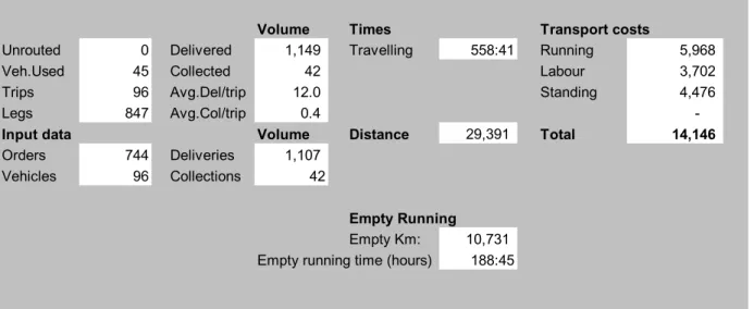
3.5.2Results of the Routing Analysis 3.5.2Results of the Routing Analysis Scenario 0 (Original situation)
The figures of the actual delivery operation were obtained from the 2002 KPI data base and costed using the data in Table 3.1.
In Table 3.2, it is shown that there are 744 orders with valid information recorded in the database. These orders are composed of 42 pallets of collections and 1,107 pallets of deliveries over the two-day period for the sample fleets involved in tertiary distribution. These customer requirements were achieved using 96 trips. These trips are mostly multiple drops/collections rounds, with an average of about 9 journey legs per trip.
Table 3. 2 . Operating and Cost Parameters for the Actual Delivery Operation
Volume Times Transport costs
Unrouted 0 Delivered 1,149 Travelling 558:41 Running 5,968 Veh.Used 45 Collected 42 Labour 3,702 Trips 96 Avg.Del/trip 12.0 Standing 4,476 Legs 847 Avg.Col/trip 0.4 -Input data Volume Distance 29,391 Total 14,146 Orders 744 Deliveries 1,107
Vehicles 96 Collections 42
Empty Running Empty Km: 10,731 Empty running time (hours) 188:45
(Note: As discussion in Section 5, the transport KPI trip audit does not specify the number of vehicles deployed on a particular delivery operation. The figure of 45 vehicles has been
estimated on the basis of the average ratio of vehicles to delivery times for the seven scenarios modelled using the Optrak package.)
On average, 12 pallets are delivered on each trip whereas only 0.4 pallets are collected. It is also shown that vehicles travelled a total of 29,391 kilometres in making these deliveries and collections, and spent 558 hours on the road. More than a third of the distance travelled was empty running (10,731 kms). The total empty running cost was £6,711, which was more than a third of the total transport cost (£19,408).
Apparently there is large potential for these fleets to improve their transport efficiency. Whether this can be achieved using optimisation software and the relaxation of scheduling constraints is tested in the following scenarios.
Scenario 1 (Base Scenario)
Using industry standard parameters, we can establish the base scenario. As explained previously, in the base scenario, the driving time is assumed to be 9 hours, and the opening time is assumed to be between 6:00 and 18:00. The delivery time window is assumed to be a period between 6 hours before and 4 hours after the scheduled arrival time. By comparing the simulation results of the other scenarios from 2 to 7 with this scenario, it will be shown how fleets’ performance can be affected by changes in scheduling constraints.
Table 3. 3 . Modelling Results for the Base Scenario (Scenario 1)
Volume Times Transport costs
Unrouted 3 Delivered 1,102 Travelling 403:02 Running 4,932
Veh.Used 37 Collected 42 Waiting 02:18 Labour 2,672
Trips 88 Avg.Del/trip 12.5 Loading 206:59 Standing 3,681
Shifts 70 Avg.Col/trip 0.5 Total 612:19
-Input data Volume Distance 24,290 Total 11,285
Orders 744 Deliveries 1107
Vehicles 96 Collections 42
Empty Running Empty Km: 8,956 Empty running time (hours) 134:28
It is shown in Table 3.3 that there are 3 unrouted orders (including 2 orders with wrong postcodes). Altogether, 88 trips and (37 vehicles) are used in this scenario. Compared with the
actual situation, this saved 8 trips. Transport cost was reduced from £19,408 to £16,351, a 16% reduction. It is worth noting that a 56% reduction in total empty running cost was also achieved.
The distribution of optimised trips in the Base Scenario can be mapped using Optrak’s trip path option (see Figure C.1 in Appendix C). Each driver’s work for the scheduling period can also be displayed as bar chart using Optrak’s trip histogram function as shown in Figure C.2 in Appendix C.
Scenario 2
By extending the driving hour by 1 hour, it is expected that some trips can be saved and the total transport cost can be reduced. This is confirmed by the simulation results of scenario 2 (Table 3.4).
Transport cost is further reduced to £16,068. Compared with the optimised base scenario, a 2% reduction in transport cost and a 5% reduction in empty running cost are possible.
Table 3. 4 . Modelling Results for Scenario 2
Volume Times Transport costs
Unrouted 4 Delivered 1,089 Travelling 393:18 Running 4,821
Veh.Used 35 Collected 42 Waiting 06:21 Labour 2,607
Trips 86 Avg.Del/trip 12.7 Loading 205:41 Standing 3,482
Shifts 67 Avg.Col/trip 0.5 Total 605:20
-Input data Volume Distance 23,741 Total 10,910
Orders 744 Deliveries 1107
Vehicles 96 Collections 42
Empty Running Empty Km: 8,481 Empty running time (hours) 129:17
Scenario 3
Scenario 3 is characterised by shorter drivers’ shifts. As shown in the optimised results (Table 3.5), shorter driving time leads to increased an number of unrouted orders, the number of vehicle used and trip numbers. It also leads to a significant increase (by 12% compared with the base scenario) in distance run empty.