Signature Sequence of
Intersection Curve of Two Quadrics for
Exact Morphological Classification
Changhe TuShandong University Wenping Wang
University of Hong Kong Bernard Mourrain INRIA
and Jiaye Wang
Shandong University
Computing the intersection curve of two quadric surfaces is an important problem in geomet-ric computation, ranging from shape modeling in computer graphics and CAD/CAM, collision detection in robotics and computational physics, to arrangement computation in computational geometry. We present the solution to the fundamental problem of complete classification of mor-phologies of the intersection curve of two quadrics (QSIC) inPR3, 3D real projective space. We show that there are in total 35 different QSIC morphologies with non-degenerate quadric pencils. For each of these 35 QSIC morphologies, through a detailed study of the eigenvalue curve and the index function jump we establish a characterizing algebraic condition expressed in terms of the Segre characteristics and the signature sequence of a quadric pencil. We show how to compute a signature sequence with rational arithmetic so as to exactly classify the morphology of the inter-section curve of any two given quadrics. Two immediate applications of our results are the robust topological classification of QSIC in computing B-rep surface representation in solid modeling and the derivation of algebraic conditions for collision detection of quadric primitives.
Categories and Subject Descriptors: I.3.5 [Computer Graphics]: Computational Geometry and Object Modeling—Curve, surface, solid, and object representations; J.6 [Computer-Aided Engineering]: Computer-aided design (CAD)
General Terms: surface-surface intersection, robust computation
Additional Key Words and Phrases: intersection curves, quadric surfaces, signature sequence, index function, morphology classification, exact computation
1. INTRODUCTION
Quadric surface, being the simplest curved surfaces, are widely used in computational science for shape representation. It is therefore often necessary to compute the intersection or detect the interference of two quadrics. In computer graphics and CAD/CAM, the intersection curve of two quadrics needs to be found for computing a boundary representation of a 3D shape defined by quadrics. In robotics [Rimon and Boyd 1997] and computational physics [Lin and Ng 1995; Perram et al. 1996] one often needs to perform interference Correspondence author’s address: Wenping Wang, Department of Computer Science, The University of Hong Kong, Pokfulam Road, Hong Kong, China. The work of the second author was partially supported by a CRCG grant from The University of Hong Kong.
analysis between ellipsoids modeling the shape of various objects. There have recently been rising interests in computing the arrangements of quadric surfaces in computational geometry [Mourrain et al. 2005; Berberich et al. 2005], a field traditionally focused on linear primitives.
The intersection curve of two quadric surfaces will be abbreviated as QSIC. Exact determination of the morphology of a QSIC is critical to the robust computation of its parametric description. We study the problem of classifying the morphology of a QSIC inPR3(3D real projective space), which means computing the structural information of the QSIC, such as the number of connected or irreducible components, the reducibility, and the type of singular points, etc. There are many types of QSIC inPR3[Sommerville 1947]. A nonsingular QSIC can have zero, one, or two components. When a QSIC is singular, it can be either irreducible or reducible. A singular but irreducible QSIC may have three different types of singular points, i.e., acnode, cusp, and crunode, while a reducible QSIC may be planar or nonplanar. A planar QSIC consists of only lines or conics, which are planar curves, while a reducible but non-planar QSIC always consists of a real line and a real space cubic curve. Among planar QSICs, further distinction can be made according to how many of the linear or conic components are imaginary, i.e., not present in the real projective space.
There are mainly three basic issues in studying the morphology of a QSIC: 1) Enumeration: listing all possible morphologically different types of QSICs; 2)Classification: determining the morphology of the QSIC of two given quadrics; 3)Representation: determining the transformation which brings a given problem QSIC into a canonical representative of its class. The first two problems are solved in this paper – we enumerate all 35 different morphologies of QSIC, and characterize each of these morphologies using a signature sequence that can exactly be computed using rational arithmetic. The third problem, not handled here, leads to a lengthy case by case study which depends a lot on the application behind.
Consider the intersection curve of two quadrics given by A: XTAX = 0 and B: XTBX = 0, where
X = (x, y, z, w)T ∈PR3andA, Bare 4×4 real symmetric matrices. Thecharacteristic polynomialofAand Bis defined as
f(λ) = det(λA−B), (1)
andf(λ) = 0 is called thecharacteristic equationofAandB.
The characteristic polynomialf(λ) is defined with a projective variableλ∈PR; thus it is either a quartic polynomial or vanishes identically. The latter case of f(λ) vanishing identically occurs if and only if A
and B are two singular quadrics sharing a singular point; thus, all the quadrics in the pencil formed byA
and B are singular. In this case, the pencil of A and B is said to be degenerate; otherwise, the pencil is non-degenerate. For example, ifAandBare two cones with their vertices at the same point, then they form a degenerate pencil. When two quadrics form a degenerate pencil, by projecting the two quadrics from one of their common singular points to a plane P not passing through the center of projection, we reduce the problem of computing the QSIC to one of computing the intersection of two conics in the planeP, which is a separate and relatively simple problem. For this reason and the sake of space, we will not cover this case in the present paper. Hence, we assume throughout thatf(λ) does not vanish identically.
Our contributions are as follows. We consider a new characterization of the QSIC of a pencil, namely the signature sequence, and show how it can be computed effectively and efficiently, using only rational arithmetic operations. We establish a complete correspondence among the QSIC morphologies, the Segre characterization over the real numbers, the Uhlig’s normal form [Uhlig 1976] and the signature sequence, which allows us to derive a direct algorithm based on exact arithmetic for the classification of QSIC. Based on this correspondence, a simplified analysis of the morphology of different QSIC’s is described. We obtain a complete table of all the possible morphologies of QSIC, with their Segre characterizations, signature se-quences and Uhlig’s normal forms. These results apply to any quadric pencil whose characteristic polynomial
f(λ) does not vanish identically. The case of f(λ)≡ 0 leads to the classification of conics inPR2, which
non-degenerate quadric pencils. A detailed explanation of these tables is given in Section 2.7.
A few words are in order about our approach. Since any pair of quadrics can be put in the Uhlig normal form, we obtain all possible QSIC morphologies by an exhaustive enumeration of all Uhlig normal forms, with distinct Jordan chains and sign combinations. For each pair of the Uhlig normal forms, on one hand, we obtain its index sequence, and on the other hand, we determine its corresponding morphology. The derivation of the index sequence necessitates the study on eigenvalue curves and index jumps at real roots of a characteristics equation, while the determination of the QSIC morphology is largely based on case-by-case geometric analysis of two quadrics in their Uhlig normal forms. Finally, we convert all index sequences to their corresponding signature sequences for efficient and exact computation. In this way we establish a complete correspondence among the QSIC morphologies, Uhlig’s normal forms and signature sequences.
The remainder of the paper is organized as follows. We discuss related work in the rest of this section. Uhlig’s method and other preliminaries, including a careful study of the eigenvalue curves of a quadric pencil, are introduced in Section 2. For an organized presentation, characterizing conditions for different QSIC morphologies are grouped into three sections: nonsingular QSIC (Section 3), singular but non-planar QSIC (Section 4), and planar QSIC (Section 5). In Section 6 we discuss how to use the obtained results for complete classification of QSIC morphologies. We conclude the paper in Section 7.
1.1 Related work
Literature on quadrics abounds, including both classical results from algebraic geometry and modern ones from computer graphics, computer-aided geometric design (CAGD) and computational geometry. Classifying the QSIC is a classical problem in algebraic geometry, but the solutions found therein are given inPC3 (3D
complex projective space), and therefore provide only a partial solution to our classification problem posed in PR3. Some methods for computing the QSIC in the computer graphics and CAGD literature do not classify the QSIC morphology completely, while others use a procedural approach to computing the QSIC morphology. The procedural approach is usually lengthy, therefore prone to erroneous classification if floating point arithmetic is used or leading to exceedingly large integer values or complicated algebraic numbers if exact arithmetic is used.
When the input quadrics are assumed to be the so-callednatural quadrics, i.e., special quadrics including spheres, circular right cones and cylinders, there are several methods that exploit geometric observations to yield robust methods for computing the QSIC [Miller 1987; Miller and Goldman 1995; Shene and Johnstone 1994]. However, we shall consider only methods for computing the QSIC of twoarbitraryquadrics, and focus on how these methods classify the QSIC morphology.
In algebraic geometry the QSIC morphology is classified inPC3 using the Segre characteristic [Bromwich 1906]. The Segre characteristic is defined by the multiplicities of the roots of f(λ) = 0 with respect to
f(λ) as well as the sub-determinants of the matrixλA−B. The Segre characteristic assumes the complex field, i.e., assuming that the input quadrics are defined with complex coefficients, and therefore it does not distinguish whether a root of f(λ) = 0 is real or imaginary. When applying the Segre characteristic in
PR3, several different types of QSICs in PR3may correspond to the same Segre characteristic, thus cannot
be distinguished. An example is the case where four morphologically different types of nonsingular QSICs correspond to the same Segre characteristic [1111], meaning thatf(λ) = 0 has four distinct roots; (see cases 1 through 4 in Table 1). In this paper we obtain a complete classification by further considering whether a root off(λ) = 0 is real or imaginary and the signature sequence of a quadric pencil.
A well-known method for computing QSIC in 3D real space is proposed by Levin [Levin 1976; 1979], based on the observation that there exists a ruled surface in the pencil of any two distinct quadrics inPR3. Levin’s method substitutes a parameterization of this ruled quadric to the equation of one of the two input quadrics to obtain a parameterization of the QSIC. However, this method does not classify the morphology of the
QSIC; consequently, it does not produce a rational parameterization for a degenerate QSIC, which is known to be a rational curve or consist of lower-degree rational components.
There have been proposed several methods that improve upon Levin’s method. Sarraga [Sarraga 1983] refines Levin’s method in several aspects but does not attempt to completely classify the QSIC. Wilf and Manor [Wilf and Manor 1993] combine Levin’s method with the Segre characteristic to devise a hybrid method, which, however, is still not capable of completely classifying the QSIC inPR3; for example, the four different types of nonsingular QSICs are not classified in PR3. Wang, Goldman and Tu [Wang et al. 2003] show how to classify the QSICs within the framework of Levin’s method. DuPont et al [Dupont et al. 2003] proposed a variant of Levin’s method in exact arithmetic by selecting a special ruled quadric in the pencil of two quadrics, in order to minimize the number of radicals used in representing the QSIC; an implementation of this method is described in [Lazard et al. 2004]. The methods in [Wang et al. 2003] and [Dupont et al. 2003] both adopt a lengthy procedural approach, with no systematic approach for a complete classification. The work of Ocken et al [Ocken et al. 1987] and Dupont’s recent Ph.D thesis [Dupont 2004] both use simultaneous matrix diagonalization [Uhlig 1976] to obtain canonical forms of two input quadrics. This diagonalization is actually computed in their methods in a procedural approach for computing the QSIC; in contrast, we use the simultaneous diagonalization as a proof technique to establish our results. Dupont gives a complete procedure to determine the type of a QSIC, covering also the case where the characteristic polynomial vanishes identically. The analysis in [Ocken et al. 1987] is incomplete, leaving some cases of QSIC morphology missing and some other cases classified incorrectly; for example, the case of a QSIC consisting of a line and a space cubic curve is missing and the cases wheref(λ) = 0 has exactly two real roots or four real roots are not distinguished.
A different idea of computing the QSIC, again using a procedural approach, is to project a QSIC into a planar algebraic curve and analyze this projection curve to deduce the properties of the QSIC, including its morphology and parameterization. Farouki, Neff and O’Connor [Farouki et al. 1989] project a QSIC to a planar quartic curve and factorize this quartic curve to determine the morphology of the QSIC. (Note that only degenerate QSICs are considered in [Farouki et al. 1989].) Wang, Joe and Goldman [Wang et al. 2002] project a QSIC to a planar cubic curve using a point of the QSIC as the center of projection; this cubic curve is then analyzed to compute the morphology and parameterization of the QSIC. However, exact computation is difficult with this method, since the center of projection is computed with Levin’s method.
A direct application of the above procedural methods is prone to relatively large accumulated errors with floating point implementation or tends to generate complicated algebraic numbers when using exact arith-metic. It is therefore natural to ask if it is possible to determine the morphology of a QSIC by checking some simple algebraic conditions, rather than invoking a long computational procedure. Algebraic conditions have recently been established for QSIC morphologies or the configuration formed by two quadrics in some special cases. A condition in terms of the number of positive real roots of the characteristic equationf(λ) is given by Wang et al in [Wang et al. 2001] for the separation of two ellipsoids in 3D affine space. Algebraic conditions are obtained by Wang and Krasauskas in [Wang and Krasauskas 2004] for non-degenerate configurations formed by two ellipsoids, and for the four types of non-singular intersection curves of two general quadrics by Tu et al in [Tu et al. 2002]. The conditions for the four cases treated in [Tu et al. 2002] are only given in terms of the number of real roots off(λ) = 0; moreover, two of the four types are not distinguished, i.e., they are covered by the same condition.
Finally, we should mention that Chionh, Goldman and Miller [Chionh et al. 1991] uses multivariate resultants to compute the intersection of three quadrics.
Table I. Classification of nonplanar QSIC inPR3
[Segre]r
r= the # Index Signature Sequence Illus- Representative of real roots Sequence tration Quadric Pair
[1111]4 1 h1|2|1|2|3i (1,(1,2),2,(1,2),1,(1,2),2,(2,1),3) A: x2+y2+z2−w2= 0 B: 2x2+ 4y2−w2= 0 2 h0|1|2|3|4i (0,(0,3),1,(1,2),2,(2,1),3,(3,0),4) A: x2+y2+z2−w2= 0 B: 2x2+ 4y2+ 3z2−w2= 0 [1111]2 3 h1|2|3i (1,(1,2),2,(2,1),3) A: 2xy+z2+w2= 0 B: −x2+y2+z2+ 2w2= 0 [1111]0 4 h2i (2) BA:: −xyx2++zwy2= 0−2z2+zw+ 2w2= 0 5 h2oo−2|3|2i h2oo+2|3|2i (2,((2,1)),2,(2,1),3,(2,1),2) (2,((1,2)),2,(2,1),3,(2,1),2) A: x 2−y2+z2+ 4yw= 0 B: −3x2+y2+z2= 0 [211]3 6 h1oo−1|2|3i (1,((1,2)),1,(1,2),2,(2,1),3) A: −x 2−z2+ 2yw= 0 B: −3x2+y2−z2= 0 7 h1oo+1|2|3i (1,((0,3)),1,(1,2),2,(2,1),3) A: x 2+z2+ 2yw= 0 B: 3x2+y2+z2= 0 [211]1 8 h2oo−2i (2,((2,1)),2) A: xy+zw= 0 B: 2xy+y2−z2+w2= 0 [22]2 9 h2oo−2oo−2i h2oo−2oo+2i (2,((2,1)),2,((2,1)),2)(2,((2,1)),2,((1,2)),2) A: xy+zw= 0 B: y2+ 2zw+w2= 0 [22]0 10 h2i (2) A: xw+yz= 0 B: xz−yw= 0 [31]2 11 h1ooo+2|3i (1,(((1,2))),2,(2,1),3) A: y 2+ 2xz+w2= 0 B: 2yz+w2= 0 [4]1 12 h2oooo−2i (2,((((2,1)))),2) A: xw+yz= 0 B: z2+ 2yw= 0 2. PRELIMINARIES 2.1 Simplification techniques
There are two transformations that we will use frequently to simplify the analysis of a QSIC. Based on Uhlig’s results on simultaneous diagonalization [Uhlig 1976] (see also Section 2.3), we sometimes apply a projective transformation to bothAandBto get a pair of quadricsA0:XT(QTAQ)X = 0 andB0 :XT(QTBQ)X= 0 in simpler forms. The transformed quadricsA0 andB0are projectively equivalent toAandB, therefore have the same QSIC morphology inPR3 and the same characteristic equation as the pairAandB.
We sometimes also consider two simpler quadrics in the pencil spanned byA andB. Note that any two distinct members of the pencil have the same QSIC as that ofAandB, and their characteristic polynomial is only different from that ofAandBby a projective (i.e., rational linear) variable substitution.
2.2 Open curve components
If a connected or an irreducible componentC of a QSIC is intersected by all planes inPR3, thenC is called
anopen component; otherwise,C is called aclosed component. Whether a curve component is open or closed is a projective property, i.e., this property is not changed by a projective transformation to the curve.
Table II. Classification of planar QSIC inPR3 - Part I
[Segre]r
r= the # Index Signature Sequence Illus- Representative of real roots Sequence tration Quadric Pair
13 h2||2|1|2i (2,((1,1)),2,(1,2),1,(1,2),2) A: x2−y2+z2−w2= 0 B: x2−2y2= 0 [(11)11]3 14 h1||3|2|3i (1,((1,1)),3,(2,1),2,(2,1),3) A: −x2+y2+z2+w2= 0 B: −x2+ 2y2= 0 15 h1||1|2|3i (1,((0,2)),1,(1,2),2,(2,1),3) A: x2+y2+z2−w2= 0 B: x2+ 2y2= 0 16 h0||2|3|4i h1||3|4|3i (0,((0,2)),2,(2,1),3,(3,0),4) (1,((1,1)),3,(3,0),4,(3,0),3) A: x 2+y2−z2−w2= 0 B: x2+ 2y2= 0 [(11)11]1 17 h1||3i (1,((1,1)),3) A: x2+y2+ 2zw= 0 B: −z2+w2+ 2zw= 0 18 h2||2i (2,((1,1)),2) A: x2−y2−2zw= 0 B: −z2+w2+ 2zw= 0 [(111)1]2 19 h1|||2|3i (1,(((0,1))),2,(2,1),3) A: y2+z2−w2= 0 B: x2= 0 20 h0|||3|4i (0,(((0,1))),3,(3,0),4) A: y2+z2+w2= 0 B: x2= 0 [(21)1]2 21 h1oo−|2|3i (1,(((1,1))),2,(2,1),3) A: y2−z2+ 2zw= 0 B: −x2+z2= 0 22 h1oo+|2|3i (1,(((0,2))),2,(2,1),3) A: y 2−z2+ 2zw= 0 B: x2+z2= 0
obtained by designating a plane inPR3that does not intersectCas the plane at infinity. For example, a real non-degenerate conic C is closed inPR3. In contrast, an open component curve is unbounded in any affine realization of PR3; a real line, for example, is an open curve inPR3. We will see some higher order open curve components occurring in several QSIC morphologies.
2.3 Simultaneous block diagonalization
When given two arbitrary quadrics, we use a projective transformation to simultaneously map the two quadrics to some simpler quadrics having the same QSIC morphology and the same root pattern of the characteristic equation. Such a projective transformation is based on the standard results on simultaneous block diagonalization of two real symmetric matrices [Uhlig 1976], which will be reviewed below.
Table III. Classification of planar QSIC inPR3- Part II
[Segre]r
r= the # Index Signature Sequence Illus- Representative of real roots Sequence tration Quadric Pair
23 h2oo−2||2i (2,((2,1)),2,((1,1)),2) A: 2xy−y2= 0 B: y2+z2−w2= 0 [2(11)]2 24 h1oo−1||3i (1,((1,2)),1,((1,1)),3) A: 2xy−y2= 0 B: y2−z2−w2= 0 25 h1oo+1||3i (1,((0,3)),1,((1,1)),3) A: 2xy−y 2= 0 B: y2+z2+w2= 0 [(31)]1 26 h2ooo−|2i (2,((((1,1)))),2) A: y2+ 2xz−w2= 0 B: yz= 0 27 h1ooo+|3i (1,((((1,1)))),3) A: y2+ 2xz+w2= 0 B: yz= 0 28 h2||2||2i (2,((1,1)),2,((1,1)),2) A: x 2−y2= 0 B: z2−w2= 0 [(11)(11)]2 29 h0||2||4i (0,((0,2)),2,((2,0)),4) A: x 2+y2= 0 B: z2+w2= 0 30 h1||1||3i (1,((0,2)),1,((1,1)),3) A: x 2+y2= 0 B: z2−w2= 0 [(11)(11)]0 31 h2i (2) BA:: −xyx2++zwy2= 0−z2+w2= 0 [(211)]1 32 h2oo−||2i (2,((((1,0)))),2) A: x 2−y2+ 2zw= 0 B: z2= 0 33 h1oo−||3i (1,((((1,0)))),3) A: x2+y2+ 2zw= 0 B: z2= 0 [(22)]1 34 h2boo−boo−2i (2,((((2,0)))),2) A: xy+zw= 0 B: y2+w2= 0 35 h2boo−boo+2i (2,((((1,1)))),2) A: xy−zw= 0 B: y2−w2= 0
Definition 1: Let AandB be two real symmetric matrices withAbeing nonsingular. ThenAandB are called anonsingular pair of real symmetric (r.s.) matrices.
Definition 2: A square matrix of the form
M = λ e . . . e λ k×k
is called a Jordan block of type Iif λ∈ R and e= 1 fork ≥2 or M = (λ) with λ∈R fork = 1; M is called aJordan block of type II if
λ= µ a −b b a ¶ a, b∈R, b6= 0 and e= µ 1 0 0 1 ¶ , fork≥4 or M = µ a −b b a ¶ fork= 2, witha, b∈R,b6= 0.
Definition 3: LetJ1,...,Jkbe all the Jordan blocks (of type I or type II) associated with the same eigenvalue
λof a real matrixA. Then
C=C(λ) = diag(J1, ..., Jk),
wheredim(Ji)≥dim(Ji+1), is called thefull chain of Jordan blocksorfull Jordan chain of lengthkassociated
with λ.
Definition 4: Ifλ1,...,λk are all distinct eigenvalues of a real matrixA, with only one being listed for each pair of complex conjugate eigenvalues, then thereal Jordan normal form of Ais J=diag(C(λ1),...,C(λk)).
Recall that two square matrices C andD are congruent if there exists a nonsingular matrixQsuch that
C =QTDQ; we also say that C and D are related by a congruence transformation, which amounts to a change of projective coordinates.
Theorem 1. (Canonical Pair Form Theorem) [Uhlig 1973a; 1976]:
LetAandBbe a nonsingular pair of real symmetric matrices of size n. Suppose thatA−1B has real Jordan
normal formdiag(J1, ...Jr, Jr+1, ...Jm), where J1, ...Jr are Jordan blocks of type I corresponding to the real eigenvalues of A−1B and J
r+1, ...Jm are Jordan blocks of type II corresponding to the complex eigenvalues of A−1B. Then the following properties hold:
(1) A andB are simultaneously congruent by a real congruence transformation to diag(ε1E1, ...εrEr, Er+1, ...Em)
and
diag(ε1E1J1, ...εrErJr, Er+1Jr+1, ...EmJm), respectively, whereεi=±1 and the Ei are of the form
0. . . .. 0 1
1 0 . 0
of the same size as Ji, i = 1,2, .., m. The signs of εi are unique for each set of indices i that are associated with a set of identical Jordan blocksJi of type I.
(2) The characteristic polynomial of A−1B and det(λA−B)have the same roots λ
j with the same multi-plicities γi.
(3) The sum of the sizes of the Jordan blocks corresponding to a real rootλiis the multiplicityγiifλiis real or twice this multiplicity ifλi is complex. The number of the corresponding blocks isρi=n−rank(λiA−B), and1≤ρi≤γi.
In order to apply Theorem 1, we need to ensure that the matrixAis nonsingular. Since we assume that
f(λ) = det(λA−B) does not vanish identically, λA−B is nonsingular for infinitely many values of λ. Therefore, given two quadricsA:XTAX = 0 andB:XTBX = 0, we may assume thatAis nonsingular; for otherwise we may replaceAby another nonsingular matrix ˜Asuch that ˜A:XTAX˜ = 0 andBhave the same QSIC as that ofAandB.
2.4 Index sequences
Signature and index: Any n×n real symmetric matrixD is congruent to a unique diagonal formD0 = diag(Ii,−Ij,0k). The signature, or inertia, of D is (σ+, σ−, σ0) = (i, j, k). The index of D is defined as
index(D) =i.
Index function: The index function of a quadric pencilλA−B is defined as Id(λ) = index(λA−B), λ∈PR.
SinceAandBare matrices of order 4 in our discussion, i.e.,n= 4, we have Id(λ)∈ {0,1,2,3,4}. Note that Id(λ) has a constant value in the interval between any two consecutive real roots off(λ) = 0. The index function may have a jump across a real root off(λ) = 0, depending on the nature of the root. The index function is also defined forλ=∞and−∞. We have Id(−∞) + Id(+∞) = rank(A).
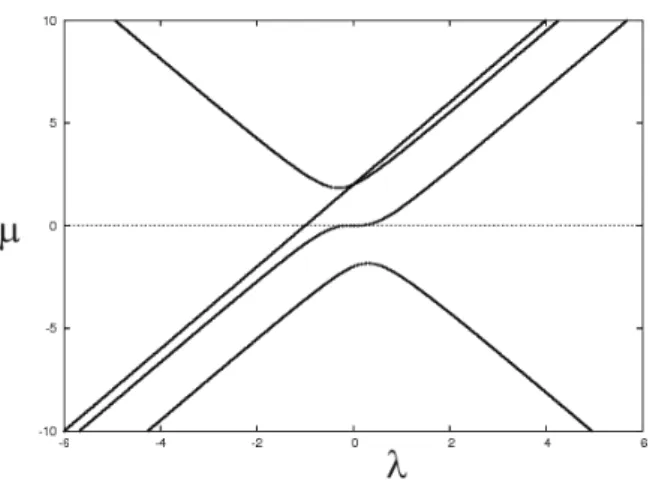
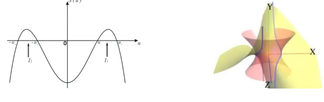
Eigenvalue Curve: We consider the real eigenvalues of the pencil λA−B, defined by the equation
C(λ, u) = det(λA−B−u I) = 0.
We are going to see that the QSIC of a pencil (A, B) can be characterized by the geometry of the planar curveCdefined by the equationC(λ, u) = 0. This curveCis defined by a polynomial whose total and partial degree in eitherλoruis 4. Since a 4×4 symmetric matrix has 4 real eigenvalues, for anyλ∈R, the number of real roots C(λ, u) = 0 in u is 4 (counted with multiplicities). Consequently, there are 4 λ-monotone branches ofC. For any fixedλ∈R, the number of points ofCnot on theλ-axis, i.e., withu6= 0, is the rank of the quadratic formλA−B; the number of points of C above the λ-axis and the number of points of C
below theλ-axis determine the signature of (λA−B). Figure 1 shows the eigenvalue curve of the pencil of quadrics (y2+ 2x z+ 1, 2y z+ 1).
Index sequence: Let λj, j = 1,2, . . . , r, be all distinct real roots off(λ) = 0 in increasing order. Let
µk,k= 1,2, . . . , r−1, be any real numbers separating theλj, i.e.,
−∞< λ1< µ1< λ2< . . . µr−1< λr<∞.
Denotesj = Id(µj), j= 1,2, . . . , r−1. Denote s0= Id(−∞) and sr= Id(∞). Then theindex sequence of
AandBis defined as
hs0↑s1↑. . .↑sr−1↑sri, where↑stands for a real root, single or multiple, off(λ) = 0.
To distinguish different types of multiplicity of a real root, we use|to denote a real root associated with a 1×1 Jordan block, and useoforpconsecutive times to denote a real root associated with ap×pJordan block. For example, a real root with Segre characteristic [11] will be denoted by|| in place of an ↑ in the index sequence, and a real root with the Segre characteristic [21] will be denoted by oo| in place of an ↑.
Fig. 1. The eigenvalue curve of the pencil of the quadrics (y2+ 2x z+ 1, 2y z+ 1).
When the Segre characteristic is (22), we useboobooto distinguish it fromoooo, which has the Segre characteristic [4]. Supposing that λ0 is a real zero off(λ) with a Jordan block of sizek×k, we useo · · · o+ or o · · · o− to indicate that the corresponding sign εi of the block in the Uhlig’s normal form is + or−.
Sinceλis a projective parameter, a projective transformationλ0 = (aλ+b)/(cλ+d) does not change the pencil but may change the index sequence of the pencil. On the other hand, thinking of the projective real line of λas a circle topologically, such a transformation induces either a rotation or a reversal of order of the index sequence of the pencil. Therefore we need to define an equivalence relation of all index sequences of a quadric pencil under projective transformations ofλ. In addition, replacing Aand B by −A and−B
changes each indexsi to rank(λA−B)−sibut essentially does not change the pencilλA−B. Note that the above replacement changes of the sign associated with a Jordan block of a root; for instance, if the quadrics
AandB have the index sequenceh2oo−2|3|2i, then−Aand−B have the index sequenceh2oo+2|1|2i.
We choose a representative in an equivalence class such that Ais nonsingular; therefore, ∞is not a root off(λ) = 0 ands0+sr= 4. Taking these observations and conventions into consideration and denoting the equivalence relation by ∼, this equivalence of index sequences is then defined by the following three rules:
1) Rotation equivalence: hs0↑s1↑. . .↑sr−1↑sri ∼ h4−sr−1↑s0↑s1↑. . .↑sr−1i, (2) hs0↑s1↑. . .↑sr−1↑sri ∼ hs1↑s2↑. . .↑sr↑4−s1i. 2) Reversal equivalence: hs0↑s1↑. . .↑sr−1↑sri ∼ hsr↑sr−1↑. . .↑s1↑s0i. (3) 3) Complement equivalence: hs0↑s1↑. . .↑sr−1↑sri ∼ h4−s0↑4−s1↑. . .↑4−sr−1↑4−sri. (4) 2.5 Signature variation
In this section we analyze the behavior of the eigenvalues of the pencil H(λ) =λA−B, near the roots of
f(λ) = det(H(λ)) = 0. This analysis amounts to analyzing the eigenvalue curves at a real root off(λ), and is needed for computing the jump of the index function at the real root.
Consider a transformationH0(λ) =PTH(λ)P ofH(λ), whereP is an invertible matrix. First, we compare the behavior of the eigenvalues ofH0(λ) and H(λ). For any real symmetric matrixQof sizen, we denote byρk(Q) the kth real eigenvalue of Q, so that ρ1(Q)6ρ2(Q) 6· · · 6ρn(Q). Using the Courant-Fischer Maximin Theorem (see [Golub and van Loan 1989] p. 403), we have the following result:
ρk(Q)σ1(P)26ρk(PTQP)6ρk(Q)σn(P)2, (5) whereσ1(P) (resp. σn(P)) is the smallest (resp. largest) singular value ofP.
Proposition 1. Let P be an invertible matrix and H0(λ) = PTH(λ)P. If ρ
k(H(λ)) = aλµ(1 +o(λ)) witha6= 0, then ρk(H0(λ)) =a0λµ(1 +o(λ))with sign(a) = sign(a0).
Proof. As the eigenvalueρk(H0(λ)) has a Puiseux expansion [Abhyankar 1990; Walker 1962] nearλ= 0 of the formρk(H0(λ)) =ρ0+a0λµ
0
(1 +o(λ)) withρ0, a0 ∈Randµ0∈Q, we deduce from the inequalities (5) thatρ0= 0,µ0 =µand sign(a0) = sign(a).
Proposition 1 allows us to deduce the behavior of the eigenvalues of the pencilH(λ), from its normal form. Indeed, by Theorem 1,H(λ) is equivalent to
D(λ) = diag(ε1E1(λI1−J1(λ1)), ε2E2(λI2−J2(λ2)), . . . , εrEr(λIr−Jr(λr)), D0(λ)), (6) where Ii is the identity matrix of the same size as that of the Jordan block Ji(λi) of eigenvalue λi, and det(D0(λ)) has no real roots. Let us denote by N
k(λ, ρ, ε) = εEk(λIk−Jk(ρ)) a block of the preceding form, wherek is the size of the corresponding matrices. Then we have the following property:
Proposition 2. The eigenvalue branchρ(λ)corresponding toNk(λ, ρ0, ε)which vanishes at λ=ρ0 is of
the form
ρ=ενk(1 +o(ν)) whereλ=ρ0+ν.
Proof. By an explicit expansion of the determinant N(λ, u) = det(Nk(λ, ρ0, ε)−uIk) and denoting
ν=λ−ρ0, we obtain
N(λ, u) =Ne(ν, u) = (−1)kuk+· · ·+ (−ε)k−1(−1)(k−1)(2k−2)+1u+εk(−1)k(k2−1)νk.
The vertices of the lower envelop of the Newton polygon ofNe(ν, u) in the (u, ν)-monomial space are the points (k,0),(1,0),(0, k). By Newton’s theorem (see [Abhyankar 1990] p. 89), the Puiseux expansion of the root branch which vanishes nearρ0 is of the form
ρ=ενk(1 +o(ν)), which completes the proof.
According to Proposition 1, if the pencilH(λ) is equivalent to (6), then near each root λi, the eigenvalue branches approaching 0 are of the formεi(λ−λi)ki(1 +o(λ−λi)), whereki is the size of a block of the Uhlig normal form (6) of the eigenvalueλi andεi is the corresponding sign.
Index Jump: The preceding analysis explains how the index function can change around the real roots off(λ) = 0. Letαbe a real root off(λ) = 0. Letα− andα+ be values sufficiently close toα, withα−< α andα+> α. Then the index jumps of Id(λ) atαare denoted as
∆−(α) = Id(α)−Id(α−), ∆+(α) = Id(α
+)−Id(α),
We denote by ∆±
i (α) the changes of signature functions of the blocksNki(λ, λi, εi) atα.Clearly, we have
∆±(α) = k X i=1 ∆± i (α), ∆(α) = k X i=1 ∆i(α). (7)
Let us describe each ∆±i (α) separately. For anya∈R, we denotea+= max(a,0) anda−= min(a,0). Note that a++a−=a.
(1) Jordan block of size1×1: In this case, clearly, we have the following signature sequence (ε−i ,(0,0), ε+i ) and the jumps are ∆−(λ
i) =ε−i ,∆+(λi) =ε+i and ∆(λi) =εi.
(2) Jordan block of size 2×2:
Nki(λ, λi, εi) =εi · 0 λ−λi λ−λi −1 ¸ .
In this case the corresponding eigenvalue branch vanishing at λi is equivalent toεi(λ−λi)2; therefore its sign is the same before and after λi. There is one positive eigenvalue and one negative eigenvalue before and after λi. If εi > 0, we have a positive eigenvalue branch which goes to 0 at λi; otherwise, we have a negative one. Thus, the signature sequence of Nki(λ, λi, εi) is (1,(1−ε
+
i ,1 +ε−i ),1) and the jumps are ∆−(λ
i) =−ε+i,∆+(λi) =ε+i and ∆(λi) = 0.
(3) Jordan block of size 3×3: Since
Nki(λ, λi, εi) =εi 00 λ−0λi λ−−1λi λ−λi −1 0 .
The corresponding eigenvalue branch is equivalent toεi(λ−λi)3, whose sign changes before and afterλi. If
εi >0, the signature ofNki(λ, λi, εi) is (1,2) beforeλi and (2,1) after. If εi<0, we exchange the order of
the two signatures. Thus, we have the signature sequence (ε+i −2ε−i ,(1,1),2ε+i −ε−i ) = (1−ε−i ,(1,1),1 +ε+i ) and ∆−(λ
i) =ε−i ,∆+(λi) =ε+i and ∆(λi) =εi.
(4) Jordan block of size 4×4: Using a similar argument, we can show that there are two positive eigenvalues and two negative eigenvalues before and after λi and the eigenvalue curve approaching zero has the form εi(λ−λi)4. Thus, the signature sequence of Nki(λ, λi, εi) is (2,(2 −ε
+
i ,2 +ε−i ),2) and ∆−(λ
i) =−ε+i,∆+(λi) =ε+i ,∆(λi) = 0.
To summarize, taking into account the signεi=±1, we have ∆i(α) =εi ifJi has the size 1×1 or 3×3, and ∆i(α) = 0 if Ji has the size 2×2 or 4×4. The rank ofH(λ) drops by 1 at λ=λi for each block of the form Nki(λ, λi, εi). Thus, the signature ofH(λi) can be deduced directly from its index Id(λi) and the
number of Jordan blocks with eigenvalueλi.
The above rules can be used to decide the permissible index jumps of Id(λ) at a real root of f(λ) = 0, through Eqn. (7) and the signature ofH(λi). In particular, in the case of a simple rootλioff(λ) = 0, the sign
εiin the Uhlig normal form can be deduced directly from the index before and after the root. For instance, an index sequence of the formh1|2|1|2|3icorresponds to a sequence of signsε1= +1, ε2=−1, ε3= +1, ε4= +1,
and the signatures at the roots are (1,2),(1,2),(1,2),(2,1), respectively.
Signature sequence: The previous analysis allows us to completely determine the signature sequence of the pencilH(λ) =λA−B, from its Uhlig normal form. For most of the cases, this signature sequence is, as we will see, a characterization of the QSIC. A signature sequence is defined as
hs0,(· · ·(p1, n1)· · ·), s1,· · ·sr−1,(· · ·(pr, nr)· · ·), sri,
where si is the index of H(λ) between two consecutive real roots of f(λ) = 0, (pi, ni) is the signature of
The advantage of using the signature sequence over using the index sequence is that we just need to compute the multiplicity of a real root and determine the signature of λA−B at the root; this is a far simpler computation than computing the Jordan block size, which is the information required by the index sequence. Conversion from an index sequence to the corresponding signature sequence is straightforward. For a given pair of quadrics, the signature sequence can be computed easily using only rational arithmetic as described in Section 2.6. Similar equivalence rules to those for index sequences apply to signature sequences as well. The signature sequences of all 35 QSIC morphologies are listed in the third column of Tables 1, 2 and 3.
2.6 Effective issues
Now we discuss how to use rational arithmetic to compute the signature sequence for classifying the QISC morphology of a given pair of quadrics. Consider the polynomial
C(λ, u) = det(λA−B−uI) =u4+c
3(λ)u3+c2(λ)u2+c1(λ)u+c0(λ).
The values where the signature changes are defined byC(λ,0) =c0(λ) =f(λ) = 0. For a fixedλ, the rank
of the corresponding quadratic form is the number of non-zero roots ofC(λ, u) = 0. For any fixed λ, the number of real roots inu, counted with multiplicity, is 4. The signature ofλA−Bis determined by the rank ofλA−B and the number of positive roots ofC(λ, u) = 0 inu. In the case where the number of real roots equals the degree of the polynomial, the Descartes rule gives an exact counting of the number of positive roots [Basu et al. 2003], and we have the following property:
Theorem 2. For anyλ∈R,
—the number of positive eigenvalues ofλA−Bis the number of sign variations of[1, c3(λ), c2(λ), c1(λ), c0(λ)].
—the number of negative eigenvalues ofλA−Bis the number of sign variations of[1,−c3(λ), c2(λ),−c1(λ), c0(λ)].
Computing the signature λA−B for λ ∈ Q is straightforward. Computing its signature at a root of
C(λ,0) = f(λ) = 0 can also be performed using only rational arithmetic. According to the previous propositions, this reduces to evaluating the sign ofci(λ),i= 1. . .3. This problem can be transformed into rational computation as follows. First, we represent a rootαoff(λ) = 0 by
—the square-free partp(λ) off(λ) = 0 and
—an isolating interval [a, b] witha, b∈Qsuch thatαis the only root ofp(λ) in [a, b].
Isolating intervals can be obtained efficiently in several ways (see, for instance, [Mourrain et al. 2005]). They can even be pre-computed in the case of polynomials of degree 4 [Emiris et al. 2004]. In order to compute the sign of a polynomialg at a root αoff(λ) = 0, we use subresultant (or Sturm-Habicht) sequences. We recall briefly the construction here and refer to [Basu et al. 2003] for more details.
Given two polynomials f(λ) and g(λ) ∈ A[λ], where A is the ring of coefficients, we compute the sub-resultant sequence inλ, defined in terms of the minors of the Sylvester resultant matrix off(λ) andf0(λ)g(λ). This yields a sequence of polynomialsR(λ) = [R0(λ), R1(λ), . . . , RN(λ)] withRi(λ)∈A[λ], whose coefficients are in the same ringA.
In our case, we takeA=Z. For anya∈R, we denote byVf,g(a) the number of sign variation of R(a). Then we have the following property [Basu et al. 2003]:
Theorem 3.
Vf,g(a)−Vf,g(b) = #{α∈[a, b] root of f(λ) = 0 whereg(α)>0} − #{α∈[a, b] root of f(λ) = 0 whereg(α)<0}.
In particular, if the interval [a, b] is an isolating interval for a rootαof c0(λ) = 0, then Vf,g(a)−Vf,g(b) gives the sign ofg(α). Takingg(λ) to be the coefficientsci(λ) in Theorem 2, this method allows us to exactly compute the signature ofαA−B, using only rational arithmetic.
Efficient implementations of the algorithms presented here are available in the librarysynaps1 and have
been applied to classifying QSIC morphologies, based on the signature sequences derived in this paper.
2.7 List of QSIC morphologies
All 35 different morphologies of QSIC are listed in Tables 1 through 3. In the first column are the Segre characteristics with the subscript indicating the number of real roots, not counting multiplicities. The index sequences and signature sequences are given in the second column and the third column, respectively. Here, only one representative is given for each equivalence class associated with the corresponding QSIC morphology; in several cases, there are two equivalence classes associated with one QSIC morphology. The numeral label for each case, from 1 to 35, is given at the left upper corner of each entry in the second column. These labels are referred to in subsequent theorems establishing the relation between the index sequence and the QSIC morphology. Cases 4, 10 and 31 share the same index sequence h2i, thus also the same signature sequence (2). Additional simple conditions based on minimal polynomials for distinguishing these three cases are presented in Section 6. Two different index sequences in cases 26 and 34 correspond to the same signature sequences; the discrimination of these two cases is also discussed in Section 6. In the illustration of each QSIC morphology in column four, a solid line or curve stands for a real component and a dashed one depicts an imaginary component. A solid dot indicates a real singular point, which in many cases is a real intersection point of two or more components of a QSIC. An open or closed component is drawn as such in the illustration. Note that, in addition to topological properties, we also take algebraic properties into consideration in defining morphologically different types. For example, a nonsingular QSIC may be vacuous in PR3, so is a QSIC consisting two imaginary conics; these two QSICs are defined to be
morphologically different since the former is irreducible algebraically but the latter is not.
3. CLASSIFICATIONS OF NONSINGULAR QSIC 3.1 [1111]4: f(λ) = 0has four distinct real roots
Theorem 4. Given two quadrics A: XTAX = 0 and B: XTBX = 0, if their characteristic equation
f(λ) = 0 has four distinct real roots, then the only possible index sequences are h1|2|1|2|3iand h0|1|2|3|4i. Furthermore,
(1) (Case 1, Table 1) when the index sequence ish1|2|1|2|3i, the QSIC has two closed components; (2) (Case 2, Table 1) when the index sequence ish0|1|2|3|4i, the QSIC is vacuous inPR3.
Proof. Let λi, i = 1,2,3,4, be the four distinct real roots of f(λ) = 0. By Theorem 1, A and B are simultaneously congruent to
¯
A= diag(ε1, ε2, ε3, ε4), and B¯ = diag(ε1λ1, ε2λ2, ε3λ3, ε4λ4),
whereεi=±1,i= 1,2,3,4. Without loss of generality, we suppose thatλ1< λ2< λ3< λ4; this permutation
of the diagonal elements can be achieved by a further congruence transformation to ¯Aand ¯B.
Clearly, the only possible index sequences are (up to the equivalence rules of Section 2.4)h1|2|1|2|3iand
h0|1|2|3|4i. Since a pencil with the second index sequenceh0|1|2|3|4icontains a positive definite or negative definite quadric, i.e., with the index being 4 or 0, we deduce that the intersection curve is empty in that case.
For the first index sequenceh1|2|1|2|3i, according to Section 2.5, the sign sequence in the corresponding Uhlig normal form is (ε1= 1, ε2=−1, ε3= 1, ε4= 1). Setting ¯AtoA0 and ¯B−λ4A¯to B0, we obtain
A0= diag(1,−1,1,1),
B0= diag ((λ1−λ4),−(λ2−λ4),(λ3−λ4),0 ).
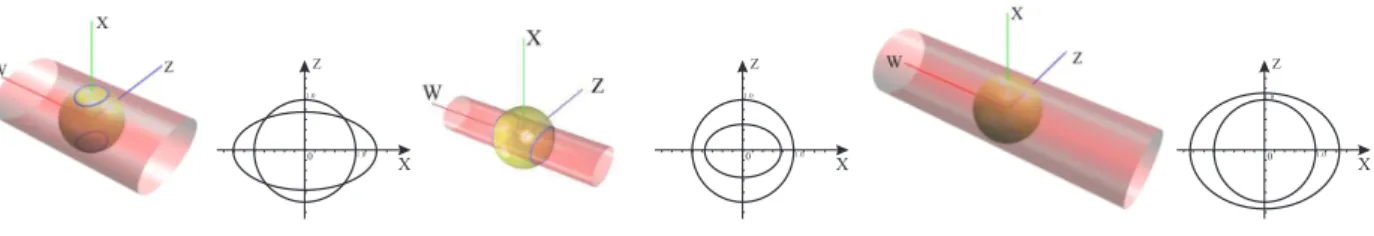
Consider the affine realization ofPR3 by making y = 0 the plane at infinity. Then A0 is a sphere, which intersects thex-zplane in a unit circle, while the quadricB0 is an elliptic cylinder with thew-axis being its central direction, which intersects thex-z plane in an ellipse, sinceλi < λ4,i= 1,2,3. Clearly, if one of the
ellipse’s semi-axes is smaller than 1 or both are smaller than 1, the QSIC ofA0andB0 has two oval branches (see the left and middle configurations in Figure 2). If both of the ellipse’s semi-axes are greater than 1,
A0 andB0 have no real intersection points (see the right configuration in Figure 2). We recall the following result from [Finsler 1937; Uhlig 1973b]: Two quadrics A: XTAX = 0andB: XTBX = 0inPR3 has no
real points if and only ifλ0A−B is positive definite or negative definite for some real numberλ0. It implies
that the index sequence of the pencil cannot be h1|2|1|2|3i. This is a contradiction. Hence, the QSIC has two ovals.
Note that none of the semi-axes can be of length 1, sincef(λ) = 0 is assumed to have no multiple roots. We deduce that the QSIC has two closed components when the index sequence ish1|2|1|2|3iand is empty when the index sequence ish0|1|2|3|4i. This completes the proof of Theorem 4.
Fig. 2. Three cases of an elliptic cylinder intersecting with a unit sphere and their corresponding cross sections in thex-zplane.
3.2 [1111]2: f(λ) = 0has two distinct real roots and a pair of complex conjugate roots
Theorem 5. (Case 3, Table 1) Iff(λ) = 0has two distinct real roots and one pair of complex conjugate roots, then the index sequence of the pencil λA−B is h1|2|3i, and the QSIC comprises exactly one closed component inPR3.
Proof. Wlog, we assumeA is nonsingular. Suppose thatf(λ) = 0 has two real roots λ16=λ2 and two
complex conjugate rootsλ3,4=a±bi. First, it is easy to see that the only index sequence possible ish1|2|3i.
We may suppose thatλ3,4=±i; this can be done by setting (B−aA)/btoB. By Theorem 1,AandB are
congruent to A0= (a0 ij) = diag(E1, ε1, ε2) = diag µµ 0 1 1 0 ¶ , ε1, ε2 ¶ , B0= (b0ij) = diag(E1J1, ε1λ1, ε2λ2) = diag(−1,1, ε1λ1, ε2λ2).
As the index sequence ish1|2|3i, we haveε1= 1, ε2= 1. Next we need consider two cases: (1)λ1λ26= 0 and
Case 1 (λ1λ2 6= 0): By a variable transformation λ0 = −λ if necessary, we may assume that at least
one of λ1 andλ2 is positive. Then we denote λ1 >0 andλ2 <0 if only one of them is positive or denote
λ2 > λ1 >0 if both are positive. It follows that λλ12 <1. We then set λ1A0−B0 to A0 and use a further
simultaneous congruence transformation to scale the diagonal elements of B0 into ±1. For simplicity of notation, we use the same symbolsA0 andB0 for the resulting matrices and obtain
A0 = (a0ij) = 1 λ1 λ1 −1 0 β2(λλ12 −1) , B0= (b0ij) = −1 1 1 β2 . whereβ2=λ2/|λ2|=±1.
Ifβ2= 1, we swap b04,4andb01,1, as well asa04,4anda01,1, to obtain
A0= (λ1 λ2 −1) −1 λ1 0 λ1 1 , B0 = 1 1 1 −1 .
Or, if β2=−1, we swapb04,4and b02,2, as well asa04,4anda02,2, to obtain
A0= 1 λ1 (1−λ1 λ2) 0 λ1 −1 , B0= −1 −1 1 1 .
Note that permuting diagonal elements can be achieved by a congruence transformation. Hence, whether
β2 = 1 or β2 = −1, after a proper simultaneous congruence transformation, B0 is the unit sphere or a
one-sheet hyperboloid with the z-axis as its central axis. Since λ1
λ2 <1, a 0
1,1 and a02,2 have the same sign.
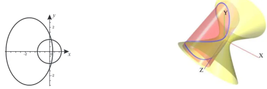
Therefore,A0 is an elliptic cylinder parallel to thez-axis. Due to the symmetry ofB0 andA0 about the x-y plane, we just need to analyze the relationship between the two conic sections in whichA0 andB0 intersect with thex-y plane.
The quadricB0 intersects thex-y plane in the unit circlex2+y2=w2, andA0 intersects thex-y plane in the ellipse x2 a2 + (y−cw)2 b2 =w 2
whenβ2= 1, or in the ellipse
(x+cw)2 b2 + y2 a2 =w 2 whenβ2=−1. Herea= q λ2(1+λ21) (λ2−λ1),b= p 1 +λ2 1, andc=λ1.
In both cases of β2 = ±1, the center of the ellipse shifts from the origin (along the x direction or y
direction) by the distance|λ1|, and the length of the ellipse’s semi-axis in the shift direction isb=p1 +λ2 1.
Then it is straightforward to verify that one of the ellipse’s extreme points of this axis is inside the unit circle, while the other is outside the unit circle. (See Figure 3 for the case of β2 = −1.) In this case the
QSIC ofA0 andB0 has one closed component inPR3(see Figure 4).
Fig. 3. The cross-sections of an elliptic cylinder and a hyperboloid with one sheet in thex-yplane.
Fig. 4. The intersection curve referred to in Figure 3 .
ε1=ε2= 1,A andB are congruent to
A0 = 0 1 1 0 1 1 , B0= −1 0 0 1 0 λ2 . First setA0−(1/λ
2)B0 to beA0. Then we use a congruence transformation to make the diagonal elements
ofB0 become±1 and apply the same transformation toA0. Denoting the resulting matrices again usingA0 andB0, we obtain A0= (a0ij) = 1 λ2 1 1 −λ1 2 1 0 , B0= (b0ij) = −1 0 0 1 0 1 . We swapb0
4,4 andb01,1, as well asa04,4 anda01,1, by a simultaneous congruence transformation to obtain
A0 = 0 −1 λ2 1 1 1 1 λ2 , B0= 1 1 0 −1 .
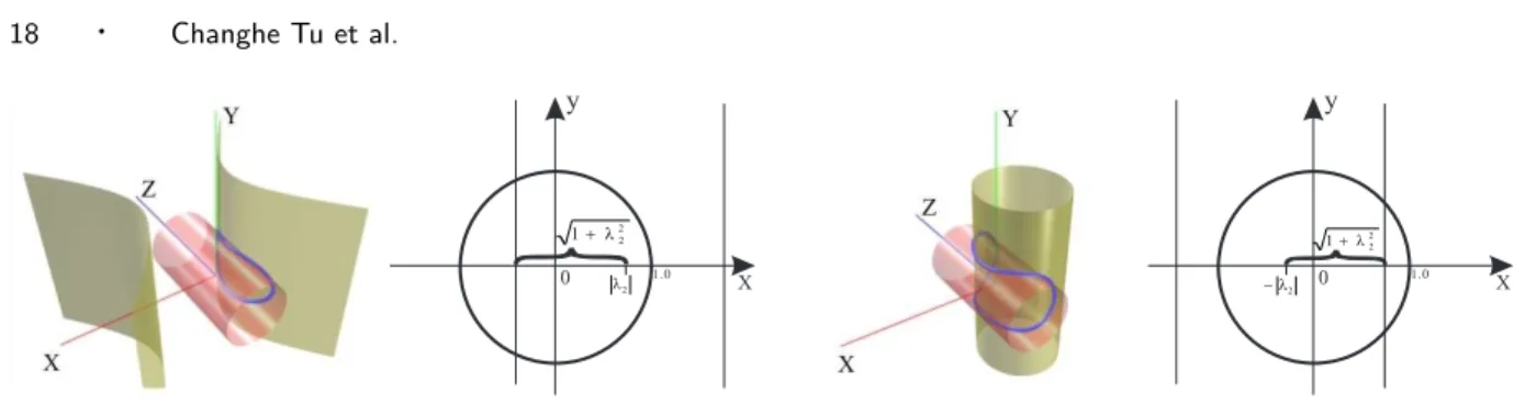
Thus,B0is a cylinder with thez-axis as its central axis, andA0 is either an elliptic cylinder or a hyperbolic cylinder, depending on the sign ofλ2, andA0 is parallel to they-axis. The equation ofA0 is
(y−cw)2 a2 ± z2 b2 =w 2, wherea=p1 +λ2 2, b= q 1+λ2 2
|λ2|, c=λ2. The cylinder A0 shifts from the origin by the distance |λ2| along thex-axis or the y-axis, and the length of its semi-axis in the shift direction is p1 +λ2
2. Clearly, in this
case, the QSIC of the cylindersA0 and B0 has exactly one closed component inPR3. (See Figure 5.) This
completes the proof.
3.3 [1111]0: f(λ) = 0has two distinct pairs of complex conjugate roots
Theorem 6. (Case 4, Table 1) Iff(λ) = 0has two distinct pairs of complex conjugate roots, then the Segre characteristic is[1111]and the index sequence ish2i. In this case the QSIC comprises two open components
Fig. 5. The intersection of a circular cylinder with a hyperbolic cylinder or an elliptic cylinder. in PR3.
Proof. Suppose that f(λ) = 0 has the roots a±bi and c±di. First, it is easy to see that the index sequence is h2i. By setting (B−cA)/d to beB, we transform conjugate rootsc±dito ±i. Therefore, we suppose that f(λ) = 0 has the roots a±biand ±i. Furthermore, we may suppose that A and B form a nonsingular pair of real symmetric matrices. Then, by Theorem 1, A and B have the following canonical forms A0= diag µµ 0 1 1 0 ¶ , µ 0 1 1 0 ¶¶ and B0 = diag µµ −1 1 ¶ , µ −b a a b ¶¶ .
Here, a6= 0 orb 6=±1, since the roots a±biare distinct from±i. Also, b6= 0 since a±biare imaginary. Wlog, we may assume b >0. In the following we will derive a parameterization of the QSIC from which the topological information about the QSIC can be deduced. The quadricA0 :XTA0X = 0 is a hyperbolic paraboloid and can therefore be parameterized byr(u, v) =g(u) +h(u)vwhere
g(u) = (−u,0,0,1)T and h(u) = (0,1, u,0)T. Substitutingr(u, v) intoXTB0X = 0 yields
v= −g(u) TB0h(u)±ps(u) h(u)TB0h(u) , (8) where s(u) = [g(u)TB0h(u)]2−[(g(u)TB0g(u))(h(u)TB0h(u))] =−bu4+ (a2+b2+ 1)u2−b.
Substituting (8) intor(u, v) yields the following parameterization of the QSIC,
p(u) = h bu3−u,− ³ au±ps(u) ´ ,−u ³ au±ps(u) ´ ,1−bu2 iT . (9)
Since p(u) is a real point only whens(u)≥ 0, we are going to identify the intervals in which s(u)≥ 0 holds. We will first show thats(u) = 0 always has four distinct real roots. The equation
s(u) =−bu4+ (a2+b2+ 1)u2−b= 0 is a quadratic equation inu2with discriminant
∆ = (a2+b2+ 1)2−4b2=a2(a2+ 2b2+ 2) + (b2−1)2>0,
sincea6= 0 orb6=±1. Therefore the two real solutions ofu2 are
u2=(a2+b2+ 1)± √
∆
![Table I. Classification of nonplanar QSIC in PR 3 [Segre] r](https://thumb-us.123doks.com/thumbv2/123dok_us/9486614.2430722/5.892.130.775.209.685/table-i-classification-of-nonplanar-qsic-pr-segre.webp)
![Table II. Classification of planar QSIC in PR 3 - Part I [Segre] r](https://thumb-us.123doks.com/thumbv2/123dok_us/9486614.2430722/6.892.149.746.201.809/table-ii-classification-planar-qsic-pr-part-segre.webp)
![Table III. Classification of planar QSIC in PR 3 - Part II [Segre] r](https://thumb-us.123doks.com/thumbv2/123dok_us/9486614.2430722/7.892.157.752.242.966/table-iii-classification-planar-qsic-pr-part-segre.webp)