University of Kentucky University of Kentucky
UKnowledge
UKnowledge
Theses and Dissertations--Computer Science Computer Science2015
Data Privacy Preservation in Collaborative Filtering Based
Data Privacy Preservation in Collaborative Filtering Based
Recommender Systems
Recommender Systems
Xiwei WangUniversity of Kentucky, [email protected]
Right click to open a feedback form in a new tab to let us know how this document benefits you. Right click to open a feedback form in a new tab to let us know how this document benefits you.
Recommended Citation Recommended Citation
Wang, Xiwei, "Data Privacy Preservation in Collaborative Filtering Based Recommender Systems" (2015). Theses and Dissertations--Computer Science. 35.
https://uknowledge.uky.edu/cs_etds/35
This Doctoral Dissertation is brought to you for free and open access by the Computer Science at UKnowledge. It has been accepted for inclusion in Theses and Dissertations--Computer Science by an authorized administrator of UKnowledge. For more information, please contact [email protected].
STUDENT AGREEMENT: STUDENT AGREEMENT:
I represent that my thesis or dissertation and abstract are my original work. Proper attribution has been given to all outside sources. I understand that I am solely responsible for obtaining any needed copyright permissions. I have obtained needed written permission statement(s) from the owner(s) of each third-party copyrighted matter to be included in my work, allowing electronic distribution (if such use is not permitted by the fair use doctrine) which will be submitted to UKnowledge as Additional File.
I hereby grant to The University of Kentucky and its agents the irrevocable, non-exclusive, and royalty-free license to archive and make accessible my work in whole or in part in all forms of media, now or hereafter known. I agree that the document mentioned above may be made available immediately for worldwide access unless an embargo applies.
I retain all other ownership rights to the copyright of my work. I also retain the right to use in future works (such as articles or books) all or part of my work. I understand that I am free to register the copyright to my work.
REVIEW, APPROVAL AND ACCEPTANCE REVIEW, APPROVAL AND ACCEPTANCE
The document mentioned above has been reviewed and accepted by the student’s advisor, on behalf of the advisory committee, and by the Director of Graduate Studies (DGS), on behalf of the program; we verify that this is the final, approved version of the student’s thesis including all changes required by the advisory committee. The undersigned agree to abide by the statements above.
Xiwei Wang, Student Dr. Jun Zhang, Major Professor Dr. Miroslaw Truszczynski, Director of Graduate Studies
DATA PRIVACY PRESERVATION IN COLLABORATIVE FILTERING BASED RECOMMENDER SYSTEMS
DISSERTATION
A dissertation submitted in partial fulfillment of the requirements for the degree of Doctor of Philosophy in the
College of Engineering at the University of Kentucky
By Xiwei Wang Lexington, Kentucky
Director: Jun Zhang, Ph.D., Professor of Computer Science Lexington, Kentucky
2015
ABSTRACT OF DISSERTATION
DATA PRIVACY PRESERVATION IN COLLABORATIVE FILTERING BASED RECOMMENDER SYSTEMS
This dissertation studies data privacy preservation in collaborative filtering based recommender systems and proposes several collaborative filtering models that aim at preserving user privacy from different perspectives.
The empirical study on multiple classical recommendation algorithms presents the basic idea of the models and explores their performance on real world datasets. The algorithms that are investigated in this study include a popularity based model, an item similarity based model, a singular value decomposition based model, and
a bipartite graph model. Top-N recommendations are evaluated to examine the
prediction accuracy.
It is apparent that with more customers’ preference data, recommender systems can better profile customers’ shopping patterns which in turn produces product rec-ommendations with higher accuracy. The precautions should be taken to address the privacy issues that arise during data sharing between two vendors. Study shows that matrix factorization techniques are ideal choices for data privacy preservation by their nature. In this dissertation, singular value decomposition (SVD) and non-negative matrix factorization (NMF) are adopted as the fundamental techniques for collaborative filtering to make privacy-preserving recommendations. The proposed SVD based model utilizes missing value imputation, randomization technique, and the truncated SVD to perturb the raw rating data. The NMF based models, namely iAux-NMF and iCluster-NMF, take into account the auxiliary information of users and items to help missing value imputation and privacy preservation. Additionally, these models support efficient incremental data update as well.
A good number of online vendors allow people to leave their feedback on products. It is considered as users’ public preferences. However, due to the connections between users’ public and private preferences, if a recommender system fails to distinguish real customers from attackers, the private preferences of real customers can be exposed. This dissertation addresses an attack model in which an attacker holds real customers’ partial ratings and tries to obtain their private preferences by cheating recommender
systems. To resolve this problem, trustworthiness information is incorporated into NMF based collaborative filtering techniques to detect the attackers and make rea-sonably different recommendations to the normal users and the attackers. By doing so, users’ private preferences can be effectively protected.
KEYWORDS: collaborative filtering, data update, matrix factorization, privacy, trustworthiness
Xiwei Wang
DATA PRIVACY PRESERVATION IN COLLABORATIVE FILTERING BASED RECOMMENDER SYSTEMS
By Xiwei Wang
Jun Zhang, Ph.D.
Director of Dissertation
Miroslaw Truszczynski, Ph.D.
Director of Graduate Studies
May 7, 2015
ACKNOWLEDGEMENTS
Upon finishing my dissertation, I would like to express my gratitude to people who encouraged, assisted, inspired, and cared about me during my PhD life at the Uni-versity of Kentucky. Without the guidance from my advisor and other committee members, help from friends, and support from my family, I would never have been able to finish my dissertation.
First of all, I would like to express my sincere appreciation to my academic advisor, Dr. Jun Zhang, for his excellent guidance, patience, encouragement, and caring. It is Dr. Zhang who led me to study the topics in privacy preserving collaborative filtering and trained me to become a researcher in this field. Because of his broad knowledge and keen professional insight, I could conduct the research in a very effective way. This allowed me to achieve promising academic success in the past six years. Dr. Zhang makes me feel at home in the United States and I am truly honored to work and study under his supervision.
Special thanks to Dr. Jinze Liu for her advice and financial support in my second academic year. Dr. Liu inspired me to read papers and start my research in the area of online recommender systems. Without her help, I would never have been able to continue my degree and begin such an interesting and meaningful research topic.
Next, I would like to thank the other faculty members of my Advisory Committee: Dr. Ruigang Yang (Department of Computer Science) and Dr. Sen-ching Cheung (Department of Electrical and Computer Engineering) for their helpful comments on my dissertation.
Then, I would like to thank my research collaborators: Dr. Yin Wang, Lawrence Technological University, for providing me with the opportunity of being a
work-shop committee member and reviewer, as well as the suggestions on writing academic papers; Dr. Nirmal Thapa, TIBCO Software Inc., for his innovative ideas and discus-sions during the first few years of my study; Mr. Kiho Lim, University of Kentucky, for his ideas on privacy-preserving vehicle communications.
Also, I would like to thank Dr. Jun Zhang, Dr. William Brent Seales, and Dr. Neil Moore for their strong recommendation letters, advice, and encouragements in my job search.
I extend my gratitude to the Elbert C. Ray eStudio for their excellent writing service. The two experts, Mr. James Marinelli and Mr. Clinton Woodson, were very friendly, easygoing, and professional. Their expertise in English writing has benefited me to a great extent. The help they provided me includes not only polishing my dissertation, but also improving my abilities in writing and speaking English.
Thanks also go to all the members in the Laboratory for High Performance Sci-entific Computing & Computer Simulation and the Laboratory for Computational Medical Imaging & Data Analysis during my study: Dr. Yin Wang, Dr. Xuwei Liang, Dr. Changjiang Zhang, Dr. Dianwei Han, Dr. Ning Cao, Dr. Nirmal Thapa, Dr. Lian Liu, Dr. Ruxin Dai, Dr. Pengpeng Lin, and Mr. Qi Zhuang. I want to thank them all for their helpful suggestions and creating a friendly working environment.
Last but not least, I would like to express my thanks and love to my parents. I thank them for giving me my life as well as their continuous support, encouragement, and endless love.
Table of Contents
Title Page 1
Abstract 2
Acknowledgements iii
Table of Contents v
List of Tables viii
List of Figures ix
1 Introduction 1
1.1 Dissertation Organization . . . 4
1.2 Related Work . . . 4
2 An Empirical Study of Recommendation Algorithms 11 2.1 Description of the Models . . . 11
2.1.1 Notational Conventions . . . 11
2.1.2 Item Popularity Based Model . . . 12
2.1.3 Item Similarity Based Model . . . 13
2.1.4 SVD Based Latent Factor Model . . . 14
2.1.5 Bipartite Graph Model . . . 15
2.2 Experimental Study . . . 17
2.2.1 Data Description . . . 17
2.2.2 Evaluation Strategy . . . 18
2.2.3 Results and Discussion . . . 19
2.2.3.1 Parameter Study . . . 19
2.2.3.2 Prediction on Datasets . . . 20
2.3 Summary . . . 25
3 SVD Based Privacy-Preserving Data Update Scheme in Collabora-tive Filtering 27 3.1 Problem Description . . . 27
3.2 Privacy-Preserving Data Update Scheme . . . 29
3.2.1 Row Update . . . 29
3.2.2 Column Update . . . 32
3.3 Experimental Study . . . 34
3.3.1 Data Description . . . 34
3.3.2 Prediction Model and Error Measurement . . . 34
3.3.3 Privacy Measurement . . . 35
3.3.4 Evaluation Strategy . . . 36
3.3.5.1 Truncation Rank (k) in SVD . . . 37
3.3.5.2 Split Ratio ρ2 . . . 38
3.3.5.3 Split Ratio ρ1 . . . 40
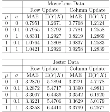
3.3.5.4 Impact of Randomization in Data Updates . . . 43
3.4 Summary . . . 45
4 Incorporating Auxiliary Information into Collaborative Filtering Data Update with Privacy Preservation 46 4.1 Problem Description . . . 47
4.2 Using iAux-NMF for Privacy-Preserving Data Updates . . . 48
4.2.1 Aux-NMF . . . 48 4.2.1.1 Objective Function . . . 48 4.2.1.2 Update Formulas . . . 51 4.2.1.3 Convergence Analysis . . . 53 4.2.1.4 Detailed Algorithm . . . 56 4.2.2 iAux-NMF . . . 57 4.2.2.1 Row Update . . . 57 4.2.2.2 Column Update . . . 58 4.3 Experimental Study . . . 58 4.3.1 Data Description . . . 58 4.3.2 Data Pre-processing . . . 59 4.3.3 Evaluation Strategy . . . 60
4.3.4 Results and Discussion . . . 62
4.3.4.1 Test on Full Training Data . . . 62
4.3.4.2 The Incremental Case . . . 65
4.3.4.3 Parameter Study . . . 68
4.4 Summary . . . 71
5 Automated Dimension Determination for NMF Based Incremental Collaborative Filtering 75 5.1 Using iCluster-NMF for Collaborative Filtering Data Updates . . . . 75
5.1.1 Clustering the Auxiliary Information . . . 76
5.1.2 Detailed Algorithm . . . 76
5.1.3 iCluster-NMF . . . 76
5.2 Experimental Study . . . 77
5.2.1 Data Pre-processing . . . 77
5.2.2 Evaluation Strategy . . . 78
5.2.3 Results and Discussion . . . 80
5.2.3.1 Parameter Setup . . . 80
5.2.3.2 Experimental Results . . . 80
5.3 Summary . . . 85
6 Trust-aware Privacy-Preserving Recommender System 89 6.1 Problem Description . . . 90
6.2 Trust-aware Privacy-Preserving Recommendation Framework . . . 92
6.2.1 Unknown Rating Predictions . . . 92
6.2.1.2 Update Formulas . . . 94
6.2.1.3 Convergence Analysis . . . 95
6.2.2 Unrelated Entries Filtering . . . 98
6.3 Experimental Study . . . 100
6.3.1 Data Description . . . 100
6.3.2 Evaluation Strategy . . . 102
6.3.3 Results and Discussion . . . 103
6.3.3.1 Privacy Preservation . . . 103
6.3.3.2 Prediction Accuracy . . . 107
6.4 Summary . . . 108
7 Conclusions and Future Work 109 7.1 Research Accomplishments . . . 109
7.2 Suggestions for Future Work . . . 112
Bibliography 117
List of Tables
2.1 Statistics of the data . . . 17
2.2 Hit rates with different α on site 5202 . . . 20
2.3 Performance list . . . 24
3.1 Impact of randomization in data updates . . . 44
4.1 Statistics of the data . . . 58
4.2 Parameter setup for Aux-NMF . . . 62
4.3 Results on MovieLens dataset . . . 64
4.4 Parameter probe on MovieLens dataset . . . 70
4.5 Parameter probe on Sushi dataset . . . 70
4.6 Parameter probe on LibimSeTi dataset . . . 70
5.1 Parameter setup for iCluster-NMF and nCluster-NMF . . . 80
5.2 Optimal number of clusters on Sushi dataset . . . 83
6.1 Statistics of the data . . . 100
6.2 Parameter setup for TrustRS . . . 103
6.3 Privacy protection level . . . 104
List of Figures
1.1 Product recommendation on Amazon.com . . . 1
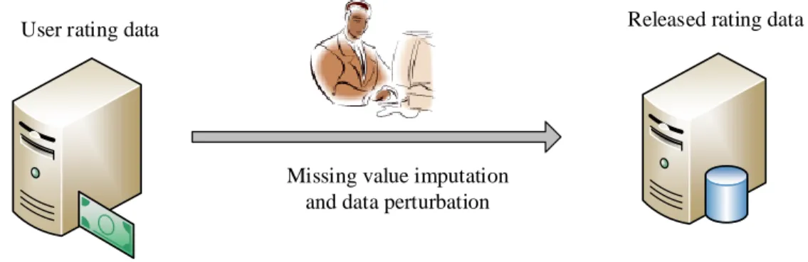
1.2 Missing value imputation and data perturbation . . . 3
2.1 A bipartite graph . . . 16
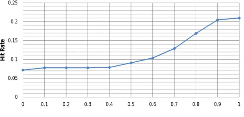
2.2 Hit rates with different γ on site 52021 . . . . 19
2.3 Hit rates in top-10 recommendation . . . 21
2.4 Hit rates in top-N recommendation . . . 25
3.1 MAE variation with different rank-k . . . 38
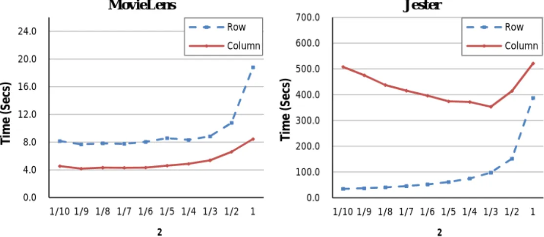
3.2 Time cost variation with split ratioρ2. . . 38
3.3 MAE variation with split ratioρ2 . . . 40
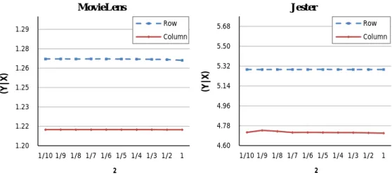
3.4 Privacy level variation with split ratio ρ2 . . . 40
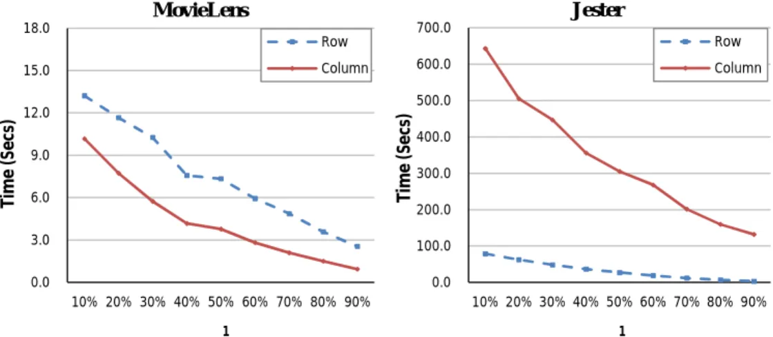
3.5 Time cost variation with split ratioρ1. . . 41
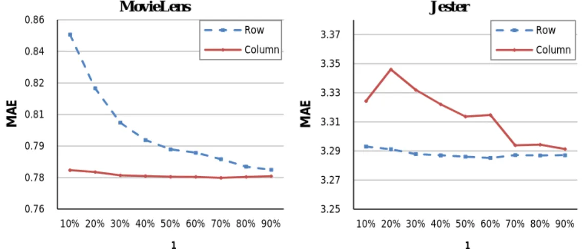
3.6 MAE variation with split ratioρ1 . . . 42
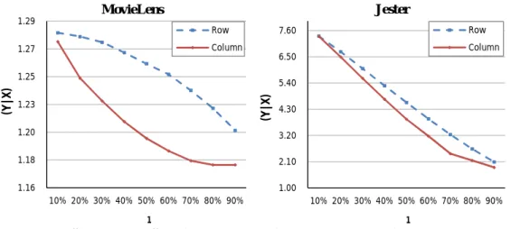
3.7 Privacy level variation with split ratio ρ1 . . . 43
3.8 Privacy loss variation with split ratioρ1 . . . 43
4.1 Updating new rows in iAux-NMF . . . 57
4.2 Clustering results on ratings predicted by Aux-NMF (a) and SVD (b) on MovieLens dataset . . . 65
4.3 Time cost variation with split ratio . . . 67
4.4 MAE variation with split ratio . . . 67
4.5 Privacy level variation with split ratio . . . 68
5.1 Time cost variation with split ratio . . . 81
5.2 MAE variation with split ratio . . . 82
6.1 An attack model . . . 92
6.2 Recall rates with varyingmu in TrustRS . . . 105
6.3 Recall rates with varying #neighbors in TrustRS . . . 106
6.4 Recall rates with varying #neighbors in PRNBC . . . 106
7.1 Incremental nonnegative tensor factorization . . . 114
1 Introduction
As technology develops, life becomes easier in many aspects. One of them is the emer-gence of electronic commerce, which not only helps sellers save resources and time but also facilitates customers in choosing and buying merchandise. Different kinds of promotions have been adopted by merchants to advertise their products. Conven-tional stores like Walmart and Sam’s Club present popular products, e.g., batteries, gift cards, and magazines at the checkout line in addition to offering discounts. This is a typical way of product recommendations. Same as conventional stores, online shops provide recommendations to their customers as well. However, for returning customers, online stores are superior to the conventional ones with respect to
prod-uct recommendations. This is due to the fact that the former have users’1 purchase
history on file which is very helpful in recommending merchandise. Online shopping websites often use recommender systems to do this task.
Figure 1.1: Product recommendation on Amazon.com
A recommender system is a program that utilizes algorithms to predict users’ purchase preferences by profiling their shopping patterns. There are many research publications about recommender systems since the mid-1990s [2]. Various approaches
1The terms “customer” and “user”are used interchangeably as they refer to the same thing in this context. This interchangeability also applies to “product” and “item”.
and models have been proposed and applied to real world applications. Most recom-mender systems are based on collaborative filtering (CF) techniques [23, 40], e.g., item/user correlation based CF’s [62], singular value decomposition (SVD) based la-tent factor CF’s [64], and nonnegative matrix factorization (NMF) based CF’s [13, 87]. With CF, previous transactions are analyzed in order to establish connections between users and products. When recommending items to a user, the CF based recommender systems try to find information related to this user to compute ratings for every possible item. Items with the highest rating scores will be presented to the user.
In many online recommender systems, it is inevitable for data owners to expose their data to other parties. For instance, due to the lack of easy-to-use technol-ogy, some online merchants buy services from professional recommendation service providers to help build their recommender systems. In addition, many shops share their real time data with business associates for better product recommendations. Such examples include two or more online bookstores that sell similar books, and on-line movie rental websites that have similar movies in their systems. In these scenar-ios, exposed data can cause privacy leakage of user information if no pre-processing is done. Typical private information includes the ratings that a user has given to particular items and on which items that this user has rated, or in general, user’s preferences. People would not like others (except the website where they purchased the products from) to know what they are interested in and to what extent they like or dislike the items. This is the most fundamental privacy problem in collaborative filtering. Thus privacy-preserving collaborative filtering algorithms [12, 59, 53] were proposed to resolve the problem. However, different from datasets for general data mining tasks, the rating matrices in collaborative filtering are typically very incom-plete, meaning that there are a large number of missing values. Accordingly, data owners should complete two tasks before releasing the data to a third party: imputing
missing ratings and perturbing the whole data.
User rating data
Missing value imputation and data perturbation
Released rating data
Figure 1.2: Missing value imputation and data perturbation
In addition, there are a few other problems and points with the CF based recom-mender systems that would be studied in this dissertation:
(1) Managing fast data growth. In the collaborative filtering context, data may grow in two aspects: the new item arrival and the new user arrival. It requires the data owners to complete the aforementioned two tasks on the new data in a timely manner. In other words, every time when the new data arrives, data owners only need to perform some incremental data update process on it and send the imputed and perturbed new data to the third parties.
(2) Utilizing auxiliary information. In some datasets, e.g., the MovieLens dataset [64], the Sushi preference dataset [35], and the LibimSeTi dating agency dataset [11], auxiliary information of users or items, e.g., users’ demographic data and items’ category data, are also provided. This information, if properly used, can improve the recommendation accuracy, especially when the original rating matrix is extremely incomplete.
(3) Distinguishing between real users and attackers with the use of social networks. It is known to people that on many online shopping websites, customers can leave feedback on the products they purchased. This is treated as users’ public preferences. Due to the connections between people’s public preferences and
private preferences, if a recommender system fails to distinguish the real customers from the attackers, it would be highly possible that the attackers can obtain users’ private preferences by cheating the system. Trustworthiness information in social networks can be used to help identify attackers for privacy preservation purposes.
1.1
Dissertation Organization
First of all, a preliminary empirical study on several collaborative filtering algorithms is presented in Chapter 2. Browsing history datasets from an American retargeting company are used as the test datasets in this study to verify their performance in binary rating data. Chapter 3 describes an SVD based privacy-preserving data up-date scheme in collaborative filtering and discusses the experimental results on the MovieLens dataset [64] and the Jester dataset [22]. An improved data update ap-proach, which adopts NMF as its fundamental technique, is proposed in Chapter 4. Chapter 5 addresses the rank determination issue that arises from the NMF based approach and shows a solution to this issue. Chapter 6 proposes an attack model in online recommender systems and presents a trust-aware privacy-preserving recom-mender system that neutralizes the attack. The future work and concluding remarks are discussed in 7.
1.2
Related Work
Collaborative filtering techniques have been extensively studied by many researchers. In [42], Yehuda divided the collaborative filtering techniques into two subareas: the neighborhood approaches and the latent factor models.
The neighborhood approaches focus on the relationships between either users or items. There are user based models [25] and item based models [18] in this scheme. For user based models, the recommendation algorithms compute the similarity
de-grees between users in order to obtain the like-minded users, i.e., the “neighbors”, of
the active users2 who will receive recommendations. Items that have been purchased
by neighbors will be recommended to this user. Thus the key point of user based neighborhood models is to find the “neighbors”. However, the computational cost of these types of models grows fast with the increasing number of users and items. With millions of users and items, it will take a substantial amount of time to compute the user similarities [18]. One way to solve this problem is to build the recommendation models based on the items. The basic principle is very close to the user based models. It attempts to compute the item-item similarity matrix and the system will recom-mend items which are similar to the ones that have been purchased by the same user in the past. Since the number of items is much smaller than the number of users in most cases, the item based models are more scalable than the user based ones. Pa-pagelis et al. [55] also showed that the former models resulted in better performance in prediction accuracy compared to the latter ones.
Different from the neighborhood approaches, the latent factor models transform users and items to the same latent factor spaces. The characteristics of users and items are “extracted” and represented at the latent level when factorizing the user-item rating matrix. The singular value decomposition (SVD) [57], the principal component analysis (PCA) [22], and the nonnegative matrix factorization (NMF) [13, 87] are three typical techniques for the latent factor models. They attempt to reduce the dimensionality of the rating matrices and utilize the reduced matrices. By doing so, noise can be decreased and some trivial factors are eliminated such that the system only retains the information that is essential to the recommendations.
However, a significant issue in most CF models is the privacy leakage. Canny [12] first proposed the privacy-preserving collaborative filtering (PPCF) that addresses this issue in the CF process. In his PPCF model, users could control all of their data.
2In many papers, the term “active users” and “test users” are used interchangeably. They both represent the users whose preferences will be predicted.
Users in a community are able to compute a public “aggregate” of their data, in which no individual user’s data is exposed. Local computation is performed by each user to get the personalized recommendations. Besides Canny’s model, the PPCF has been studied in both distributed systems [12, 84, 6, 83, 48, 65] and centralized systems [60, 47, 34, 14]. While most peer-to-peer (P2P) environments adopt dis-tributed recommender systems, centralized systems are widely used by almost all of the most popular online vendors, e.g., eBay, Amazon, and Newegg. In centralized systems, users send their data to a server and they do not participate in the CF process; only the server needs to conduct the CF. Polat and Du [59, 60] applied ran-domized perturbation techniques to the SVD based collaborative filtering to provide privacy-preserving recommendations. In their method, uniform or Gaussian noise is added to the users’ real ratings and then the server predicts the unknown ratings by the perturbed data.
In this framework, the data owner also needs to manage the fast data growth and should ensure that privacy protection is still kept at a reasonable level after the data update. Among all data perturbation methods, SVD is acknowledged as a feasible and effective data perturbation technique. Stewart [67] surveyed the perturbation theory of singular value decomposition and its application in signal processing. Brand [9] demonstrated a fast low-rank modification of the thin singular value decomposition. This algorithm can update an SVD with new rows/columns and compute its low rank approximation very efficiently. Tougas and Spiteri [72] proposed a partial SVD update scheme that requires one QR factorization and one SVD in each update. Since both factorizations are performed on small intermediate matrices, the computation cost is not expensive. Based on their work, Wang et al. [75] presented an improved SVD based data value hiding method and tested it with clustering algorithms on both synthetic datasets and real datasets. Their experimental results indicate that, by introducing the incremental matrix decomposition, the efficiency of the SVD based
data value hiding model is significantly increased. It also provides better scalability and better real-time performance of the model. The scheme proposed in Chapter 3 is similar to this model but it modifies the SVD update algorithm and comes with randomization and post-processing techniques so it can be incorporated into the SVD based CF smoothly.
In addition to SVD, NMF has also been studied in collaborative filtering. Zhang et al. [87] applied NMF to collaborative filtering to learn the missing values in the rating matrix. They treated NMF as a solution to the expectation maximization (EM) prob-lems. Chen et al. [13] proposed an orthogonal nonnegative matrix tri-factorization (ONMTF) [20] based collaborative filtering algorithm. Their algorithm also takes into account the user similarity and item similarity. To study how differently NMF would perform from SVD, based on Polat’s model [60], Li et al. [47] used NMF instead of SVD as the fundamental collaborative filtering technique and they obtained better results than Polat’s method. While both methods were demonstrated to perturb the data to a reasonable level and keep the prediction precision, it is not clear how much contribution can be made by the methods to the real world recommender systems. Different from Polat’s and Li’s work, Kaleli et al. [34] proposed a privacy-preserving naive Bayesian classifier (PPNBC) CF approach. The approach employs randomized response techniques (RRT) [76] to protect users’ privacy while producing referrals by a naive Bayesian classifier (NBC). In their scheme, the RRT is applied to both the one-group scheme and the multi-group scheme for data distortion purposes. The distorted data is then fed to NBC for recommendations. Adding to [34], Bilge et al. [8] utilized pre-processing to improve the privacy-preserving recommendations. In their method, the masked data is pre-processed by identifying the most similar items to each item off-line; some of the unrated items’ entries are also filled to improve the density. Since the increasing numbers of features and groups would degrade the online performance of the multi-group PPNBC significantly, decreasing the amount
of data involved in CF can be very beneficial. With the varying number of neighbors, the central server can decide how many items would be recommended to the users.
As mentioned before, auxiliary information of users and items is helpful if properly utilized. The fast data update approach proposed in Chapter 4 first converts this information to the cluster membership indicator matrices which are then considered as constraints for updating factor matrices. Nirmal et al. [71] proposed explicit incorporation of the additional constraint, called the “clustering constraint”, into NMF in order to suppress the data patterns in the process of performing the matrix factorization. Their work is based on the idea that one of the factor matrices in NMF contains cluster membership indicators. The clustering constraint is another indicator matrix with altered class membership in it. This constraint then guides NMF in updating factor matrices. Based on this idea, the proposed model applies the user and item cluster membership indicators to nonnegative matrix tri-factorization (NMTF), which results in better imputation of the missing values.
With regard to the clustering algorithms, K-Means [51] is a popular and well studied approach that is easy to implement and is widely used in many domains. As the name of the algorithm indicates, K-Means needs the definition of “mean” prior to clustering. It minimizes a cost function by calculating the means of clusters. This makes K-Means most suitable for continuous numerical data. When given categorical data such as users’ demographic data and movies’ genre information, K-Means needs a pre-processing phase to make the data suitable for clustering. Huang [27] proposed a K-Modes clustering algorithm to extend the K-Means paradigm to the categorical domains. Their algorithm introduces new dissimilarity measures to handle categorical objects and replaces means of clusters with modes. Additionally, a frequency based method is used to update modes in the clustering process so that the clustering cost function is minimized. In 2005, Huang et al. [28] further applied a new dissimilarity measure to the K-Modes clustering algorithm to improve its clustering accuracy.
The fast data growth requires the clustering algorithms to update the clusters constantly. The number of clusters might be increased or decreased. Su et al. [68] proposed a fast incremental clustering algorithm by changing the radius threshold value dynamically. Their algorithm restricts the number of the final clusters and reads the original dataset only once. It also considers the frequency information of the attribute values in the inter-cluster dissimilarity measure. The approach proposed in Chapter 5 adopts their clustering algorithm with some modifications. It is known that the NMF based collaborative filtering algorithms need to determine the dimensions of the factor matrices and update them when necessary. It is not convenient for people to manually specify these values and the automated decision making is highly desired. To this purpose, the proposed method determines the number of clusters by an incremental clustering algorithm and uses them as the dimensions in NMF.
Recent work on using trustworthiness in collaborative filtering indicates that this information benefits prediction precision as well as privacy protection. It reveals the trust relationships between users and can be obtained from online social networks. Jamali et al. [31] proposed SocialMF, a recommender system that makes use of the matrix factorization technique with trust propagation in social networks. Similar to [31], [80] proposed TrustMF to handle data sparsity and cold start problems which happen commonly in collaborative filtering based recommender systems. In TrustMF, users are projected into low-dimensional latent feature spaces by the matrix factoriza-tion technique according to their relafactoriza-tionships. By doing so, users’ mutual influence on their own opinions is reflected in a more reasonable way. In [33], the authors presented a trust based recommendation scheme on vertically distributed data for privacy preservation. The scheme builds a trust web of users and then uses it to filter users’ neighbors in order to protect the privacy. The proposed privacy-preserving recommender system framework in Chapter 6 incorporates trustworthiness into the weighted nonnegative matrix tri-factorizarion to improve prediction accuracy and
privacy protection.
In [48] and [65], the authors proposed group based privacy-preserving recom-mender systems in which recommendations are made at the group level as opposed to the individual level. Their experimental results show that user groups can be used as the natural protective mechanism for achieving promising privacy protection. In [48], items are grouped in terms of their ratings so users’ public interests and private interests can be separated. Then, preferences of group members are identified and aggregated. Recommendations are made by personalizing the group preferences lo-cally to conceal users’ private interests. Motivated by this framework, in Chapter 6, items and users are grouped according to the factor matrices of NMF in centralized systems to distinguish the real users from the attackers.
2 An Empirical Study of Recommendation Algorithms
In this chapter, several classical recommendation algorithms, namely the popularity based model, the item similarity based model, the SVD based model, and the bi-partite graph model, are studied on the clicking history datasets of online shopping websites collected by an American retargeting company. A massive amount of lit-erature in recommender systems examined the models on rating datasets, such as the Netflix movie rating data [4], the MovieLens dataset [64], and the Jester dataset [22]. While rating information is directly connected to people’s preferences, it is not always available. Although a majority of online shopping websites provide rating mechanisms for people to leave feedback on products, there are a few companies that might only be able to collect users’ clicking data due to technical restrictions. For example, the retargeting companies usually insert a piece of JavaScript code into the web pages of online vendors to keep track of users’ clicking behaviors. They do not have the permission to obtain or utilize data other than this. The datasets from the retargeting company contains only clicking history, e.g., a certain user clicked the link to a particular product. It is interesting to investigate the above recommendation al-gorithms on binary browsing data instead of numerical rating data with respect to prediction accuracy.
2.1
Description of the Models
2.1.1
Notational Conventions
A matrix is used to store the clicking relationships between users and items, called
the user-item rating1 matrix, denoted by R. Assume there are m users and n items,
1Although the values in this matrix are not really ratings, the matrix is still called the rating matrix for consistency.
then R∈Rm×n. An entryr
ij is the click count that user idid on item j in the given
time period. Though there is no definite proof that a user who clicks an item will buy it, a high click count may imply that the user is interested in it. Since each user may only click a few items and a single item only receives a small number of clicks,
R is incomplete, meaning that there are many missing entries.
For user i and item j, the existing click count from i to j is denoted as rij and
the predicted one is denoted aspij. The recommended items should be interesting to
the active user, i.e., this user is likely to click the recommended items.
2.1.2
Item Popularity Based Model
The item popularity based approaches are very traditional ones in recommender sys-tems. The main idea of the item popularity based models is to recommend the most popular, the most viewed, or the best selling items to users. Although the item popu-larity based models overlook users’ preferences, these kinds of models are still effective to a certain degree, and are adopted as an auxiliary component in recommender sys-tems by many famous online shopping sites, such as eBay, Amazon, etc.
The item popularity based model that is tested in this chapter maintains a
popu-larity list for each data set, denoted byL={tj}j=1,2···,n. The elements inLare items
in descending order in terms of their view counts, denoted by npj.
For the simple implementation of the popularity based top-N recommendation,
items corresponding to the firstN elements in listLwill be recommended. However,
these recommended items may not be interesting to a user, which means less accurate predictions. Thus, a further filtering step should be employed in this model to improve
the prediction accuracy. The filtering step introduces a new parameter hi into the
model, where
hi =
number of distinct items viewed by user i
The value ofhi reveals some of users’ browsing habits, such as the user preferring
to view an item just once, or preferring to view an item for several times during browsing. In the former case, the filtering step does not recommend the items that have been already viewed by the user. In the latter case, such items could also be
presented to the user. A threshold ht is set to determine whether a further filtering
step is necessary for user i:
1. if hi < ht, recommend the top-N items inL to the user;
2. if hi ≥ht, perform the filtering step.
Case 2 means the number of distinct items viewed by user i is close to the total
number of items viewed by this user. In other words, this user is not prone to click
each item multiple times. Then the items that have been clicked by user i will be
excluded from the recommendation list which is generated in the first step.
The filtering step is also applicable to other models, such as the item similarity-based model. To utilize the filtering step, other models are required to generate an
ordered top-(2N) item list for top-N recommendation. The top-(2N) list will take
the place of popularity list L.
2.1.3
Item Similarity Based Model
Among all recommender systems, the similarity based models are one of the easiest methods to implement. Papagelis et al. [55] showed that, in most cases, the item similarity based models produce better prediction accuracy than the user similarity based models. In the item similarity based model [55], when recommending items to
a user i, the system first retrieves neighbors of the items that have been viewed by
this user. It then selects the N most similar neighbors and recommends them to i.
In the real world scenarios, a notable challenge in recommender systems is the cold start problem [56]. It often occurs when users have presented very few to no
opinions. To resolve this issue, the item popularity factor is incorporated into the similarity based model to handle new users. Eq. (2.2) calculates the relationship
between user i and item j.
pij =γ· 1 |S(j;i)| X k∈S(j;i), ρjk>0 ρ2jk + (1−γ)·npj Ng (2.2)
The first tier of the equation is the similarity score and the second tier is the
popularity score. S(j;i) is the set of items that were viewed by user iand are similar
to item j. ρjk is the Pearson correlation coefficient [62] between item j and item k.
The popularity score is the ratio between the view count of item j, denoted by npj,
and the global maximum view count, denoted by Ng. γ controls the weight of each
part.
The formula for Pearson correlation coefficient is slightly modified to better de-scribe the relationship between two items.
ρjk = Pd t=1(x 0 jt−x¯j)(x0kt−x¯k) q Pd t=1(x 0 jt −x¯j)2 Pd t=1(x 0 kt−x¯k)2 , (2.3)
wherex0jt =xjt(1 +1+log1nct) is a variation ofxjt (nct is the number of items that user
i has viewed) and d is the dimensionality of an item vector xj. Note that each entry
inxj corresponds to a user’s click count on this item.
The modification on xjt is based on the premise that users who have clicked fewer
items make more contribution to the similarity computation than those who have clicked significantly more items.
2.1.4
SVD Based Latent Factor Model
The latent factor models [42] focus on reducing dimensionality of the user-item rating matrix in order to discover some “latent factors”. These factors should best interpret user preferences with the least noise. They can be exploited to approximate the
original rating values.
In Paterek’s SVD based latent factor model [57], the user-item rating matrix
is factorized into two lower rank matrices, i.e., a “user factor” matrix U F and an
“item factor” matrix IF. Thus, each user i and item j can be represented as an f
-dimensional factor vectorU Fi (i-th row ofU F) andIFj (j-th row ofIF), respectively
[15]. The prediction of the rating left by user i on item j is made by taking inner
product of U Fi and IFj.
In order to obtain the user and item factor vectors, SVD is applied on the huge
incomplete matrix R with all the missing values being set to zeros2.
Rm×n=Um×r·Sr×r·VnT×r, (2.4)
whereU andV are orthonormal matrices, S is a diagonal matrix with singular values
on its diagonal and r is the rank ofS.
With SVDLIBC (an SVD-package) [7], the dimension f (f ≤ r) can be easily
specified when decomposing the rating matrix. Hence, the user factor matrix and the item factor matrix are represented by
U Fm×f =Um×f ·
p
Sf×f, IFn×f =Vn×f ·
p
Sf×f (2.5)
and so a prediction can be made by Rij =U Fi·IFjT.
2.1.5
Bipartite Graph Model
In this graph model [26], users and items are represented as vertices of a graph and
can be divided into two disjoint sets, the item set I and the user set U. Every edge
is a connection between a vertex in U and one inI. It corresponds to an entry rij in
user-item rating matrix R, as shown in Figure 2.1.
e
1e
ie
je
nu
1u
tu
mItem Set
User Set
r
miFigure 2.1: A bipartite graph
Sets I and U in the bipartite graph model are independent sets [7]. Therefore,
the transition probability between each item pair ej and ek can be obtained by Eq.
(2.6). P(ej|ek) = m X t=1 [P(ej|ut)·P(ut|ek)], (2.6) where P(ej|ut) = rtj/ Pn i=1rti, and P(ut|ek) =rtk/ Pm t=1rtk.
All item nodes now form a finite Markov chain with transition matrix P =
[ajk]j,k=1,···,n, where ajk = P(ej|ek) [44], i.e., the probability that this chain ends
in the specific item nodeej with initial node ek is ajk. Therefore, given the previous
click history of user i, the probability for a certain item j that this user might be
interested in can be predicted according to
pij = m
X
k=1
(ejk·Tik), (2.7)
whereTi represents the initial state vector for user iin a Markov chain andTik is the
component corresponding to item k. Note that Tik =rik/Pnj=1rij.
In order to penalize the users (or items) with a large number of clicks, the
pe-nalization parameter α is introduced in the model [26, 46]. It is based on a similar
similarities. Transition probability with penalization parameter α is: P(ej|ut) = rtj/( n X i=1 rti)α, P(ut|ek) = rtk/( m X t=1 rtk)α (2.8)
2.2
Experimental Study
2.2.1
Data Description
The dataset in the experiments was gathered by a retargeting company for research purposes. It consists of the browsing history from 139 online shopping websites in one week (08/08/2010 – 08/14/2010). In the dataset, each row represents a transaction, which has four attributes, product ID, website ID, user ID, and date.
Among 139 sites, 4 were selected for test purposes. Statistics are shown in Table 2.1
Table 2.1: Statistics of the data
Site ID # of Users # of Items # of Clicks
3699 20,471 499 134,982
5202 148.409 1,004 300,757
8631 112,738 94 1,559,529
9093 70,049 2,303 120,836
Each dataset is divided into three subsets, the training set, test set and last transaction set. The training set is obtained from the original dataset by removing 1000 active users and their accompanying data. In order to ensure the items that have been viewed by active users also exist in the training set, the items should occur at least 15 times in the training set after the active users’ data has been removed. The last transactions of the removed active users form the last transaction set and the remaining data form the test set.
The goal is to train the models using the training set and apply the models on the data in the test set to predict the last transaction of the active users.
2.2.2
Evaluation Strategy
In general, there are two ways to evaluate the prediction accuracy of the
recommen-dation algorithms: hit rates (or recall rates) for top-N recommendation, and error
measurement (e.g., root mean square error and mean absolute error) for rating value predictions. Since the datasets are different from Netflix and MovieLens, which
pro-vide real ratings, it is more reasonable to make top-N recommendations rather than
rating value predictions on the clicking data. Accordingly, the prediction accuracy is evaluated in terms of the hit rates.
The recommended item set is named the predicted set. The hit rate of recom-mendations (higher is better) is calculated as follows,
hi =
number of correctly predicted active users
total number of active users (2.9)
Within the item popularity based model, an item popularity list is constructed by collecting statistics on the clicking history. The filtering step is applied on this list to obtain the final recommended items.
In the item similarity based model, the parameter γ is tweaked to get the best
ratio of similarity score and popularity score. γ is chosen from the interval of [0, 1]
with step size 0.1.
The bipartite graph model first builds a probability transition matrix with Eqs. (2.6) and (2.8). The prediction is computed based on the Markov chain in the matrix. To investigate the influence of the filtering step on other models, this step is
applied to the ordered top-(2N) recommendation lists generated by other models to
2.2.3
Results and Discussion
Prior to the comparisons of prediction accuracy, the parameters in the item based similarity model and the bipartite graph model are studied on the website with site ID 5202.
2.2.3.1 Parameter Study
(1) γ in the item based similarity model
0 0.05 0.1 0.15 0.2 0.25 0 0.1 0.2 0.3 0.4 0.5 0.6 0.7 0.8 0.9 1 H it Ra te γ
Figure 2.2: Hit rates with differentγ on site 52023
The curve in Figure 2.2 shows that withγ increasing, better hit rates are reached.
The popularity score does not seem to be more effective than the similarity score. Nevertheless, as stated before, the purpose of using the popularity score is to provide recommendations for new users who have almost no preference. In the experiments, the hit rates are tested by applying the models on users that have clicking records in both the test set and the last transaction set. This test methodology does not necessarily focus on the new user problem. Thus, the popularity score is eliminated
by setting γ to 1.0, which means this model will recommend items based on the
similarity based score only in later experiments.
(2) α in the bipartite graph model
In this model, α penalizes the users or items with lots of clicks. Therefore with
a larger α, the corresponding probabilities in Eq. (2.8) become smaller. Table 2.2
shows the hit rates with different α.
Table 2.2: Hit rates with different α on site 5202
α Hit Rate
0.5 20%
1 21.2%
2 14.2%
In the test datasets, the number of distinct items that each user has clicked does
not vary remarkably. Hence the penalization parameter α does not have significant
effects on the hit rates. Nevertheless, in grocery shopping [46], a customer purchasing a large number of a specific product reflects a higher interest in this product.
Gen-erally speaking, α = 1 is suitable for the cases in which the range of values in the
rating matrix is not wide.
2.2.3.2 Prediction on Datasets
The four models were first tested on site 3699. Figure 2.3(a) shows the hit rates. IP denotes the item popularity based model; IS denotes the item similarity based model; f-IS denotes the item similarity based model with the filtering step; BG is for the bipartite graph model; f-BG is for the bipartite graph model with the filtering step; SVD is for the SVD-based latent factor model; lastly, f-SVD is for the SVD-based latent factor model with the filtering step.
On this site, the SVD based model with 60 factors achieved the highest hit rate, which is significantly better than other models. More factors were also tested on it but no better results were obtained. This means the first 60 factors were able to capture the most critical latent properties of the items in this dataset.
0.0% 10.0% 20.0% 30.0% 40.0% 50.0% 60.0% 70.0% 80.0% 90.0% 100.0% 9.1% 40.2% 67.3% 46.7% 70.9% 90.7% 90.7% H it Ra te Model 0.0% 10.0% 20.0% 30.0% 40.0% 50.0% 60.0% 70.0% 80.0% 90.0% 100.0% 7.9% 20.5%26.4% 21.2%26.5%18.6% 18.6% H it Ra te Model
(a) Hit rates on site 3699 (b) Hit rates on site 5202
0.0% 10.0% 20.0% 30.0% 40.0% 50.0% 60.0% 70.0% 80.0% 90.0% 100.0% 98.6% 11.6%20.1%10.5%19.5% 95.9% 95.9% H it Ra te Model 0.0% 10.0% 20.0% 30.0% 40.0% 50.0% 60.0% 70.0% 80.0% 90.0% 100.0% 11.5% 27.3% 32.0%32.8% 38.3% 19.5% 19.5% H it Ra te Model
(c) Hit rates on site 8631 (d) Hit rates on site 9093
Figure 2.3: Hit rates in top-10 recommendation
The bipartite graph model reached a hit rate of 46.7%, which is close to the results of the item similarity based model. Essentially, BG has a similar principle with IS since they both need to build an item-item matrix. The difference lies on the viewpoint of entries in the matrix – transition probability in BG and item similarity in IS. In fact, some IS models obtain the similarities by computing the conditional probability between items and users.
The item popularity based model performed worst on this dataset. This is because there are 499 items but only 10 items were recommended to each active user. However, the filtering step in IP worked quite well with IS and BG. The hit rate is 67.3% for
f-IS (70.9% for f-BG) where the top-20 recommendation by the IS model made a hit rate of 67.6% (71.0% for BG). It means that almost all irrelevant items were filtered out while the correct ones were retained. The investigation on user browsing habits reveals that most users clicked distinct items just once. Therefore they may not be interested in the items they have already clicked.
It is worth mentioning that in the IS model, the neighbors of items that have been viewed by a user may have already been viewed by the same person. Accordingly, the IS based recommendation is not entirely suitable to these kinds of users and a further filtering step is needed.
Nevertheless, the filtering step had no effect on the SVD based model. It can be inferred that the latent factors in SVD not only captured the users’ click count information but also the clicking patterns, i.e., the browsing habit, so no filtering step is needed.
For the website with site ID 5202, the results charted in Figure 2.3(b) are quite different from those on 3699. All the models with filtering step except f-SVD per-formed better than others did. IS and BG, f-IS and f-BG had very similar hit rates, respectively. IP produced the worst prediction accuracy once again. However, SVD with 70 factors, the champion of the previous experiment, only achieved a hit rate of 18.6%. This indicates that the latent factors did not capture the correlations between users and items very well. The f-SVD again had no improvement on SVD.
Figure 2.3(d) presents the results on the website with site ID 9093. The bipartite graph model with filtering step performed best. SVD with 100 factors had a similar hit rate on site 5202. The results show that on some datasets, the local relationships among items that were obtained by BG and IS-like models play a more crucial role in predicting the next item. Whereas on some other datasets, capturing the global effects that were obtained by SVD-like latent factor models is more important.
dif-ferent. SVD and IP models had very high hit rates compared to others. In this case, 94 factors, which is the same as the number of items, were used in the SVD model. Note that this website has special properties – it has very few items (94) and a large number of users (112,738). Examining the recommended item list of the SVD model shows that it only generated one item for each user. In other words, the top-1 recom-mendation of SVD on this site provided correct predictions for 95.9% users. The item popularity based model performed even better since the popular items are welcomed by most users – this differs from that in the first dataset. f-SVD was not employed on this site due to the fact that there was no top-20 list for the filtering step to work on.
An interesting question remains: why did BG and IS perform significantly worse on this dataset compared to others? In [29], Huang et al. discussed the sparsity of the user-item rating matrix which can be used to answer this question. Due to the small number of items and the large number of users, most customers have only clicked a few items. Then the number of edges in the BG model connecting to these users is small. Hence, the transition probability will no longer represent the similarity of products. This also happens in the IS model – an item is similar to almost all other items with very close similarity degrees. If customers in this dataset tend to be interested in several popular items, the prediction accuracy can be very low. This also explains the positive results of the IP model in this case.
Furthermore, if the dataset has many items but very few customers who have viewed several items, the number of edges associated with most customers would be very high. Most entries in the transition matrix will then have small and close values, which will prevent the model from discovering closely related items.
As a summary of top-10 recommendations, Table 2.3 gives the performance
statis-tics of seven models4 on four datasets. The models are ranked by their hit rates –
4Since SVD and f-SVD have the same hit rates, SVD is used to represent both SVD and f-SVD in this table.
Table 2.3: Performance list Performance Rank Dataset IP IS f-IS BG f-BG SVD 3699 6 5 3 4 2 1 5202 6 4 2 3 1 5 8631 1 5 3 6 4 2 9093 6 4 3 2 1 5
the model that performs best is ranked 1 and the one which performs worst is ranked 6. It is expected that the IP model has the lowest rank (rank 6 in total) since it is only based on the popularity of items. The f-BG and f-IS models attained the first two places. SVD also worked well in most cases. It can be seen that some mod-els predicted very accurately for only certain datasets while f-BG and f-IS modmod-els had higher average hit rates than others. Thus, the models with the filtering step, which take into consideration human behavior patterns, can be employed by most recommendation tasks to achieve satisfactory results.
In the end, the hit rates with differentN’s in top-N recommendation were studied.
The predictions with seven models were performed on four sites. Figure 2.4 shows the variance.
The figures show the increasing trends with greater N for all models on all sites.
The differences lie in the slope of the curves. The models with the filtering step – f-BG
and f-IS had about 20%∼ 50% improvement in accuracy on the original models, BG
and IS. In this experiment, site 8631 is still a special one compared to others because
the hit rates of SVD and IP reached 95.9% and 98.6% whenN = 5, respectively. That
means, for these two models, the top-5 recommended items were accurately predicted and the hit rates for top-1 predictions are 95.2% and 98.5%. Consequently, on this website, the top-5 recommendations are preferable for SVD and IP models since the number of items recommended to users are expected to be small – users may not be interested in a top-50 or top-100 recommendation list as they are not helpful at all.
0.0% 10.0% 20.0% 30.0% 40.0% 50.0% 60.0% 70.0% 80.0% 90.0% 100.0% 0 5 10 15 20 IP IS f-IS BG f-BG SVD f-SVD H it Ra te N 0.0% 10.0% 20.0% 30.0% 40.0% 50.0% 60.0% 70.0% 80.0% 90.0% 100.0% 0 5 10 15 20 IP IS f-IS BG f-BG SVD f-SVD H it Ra te N
(a) Hit rates on site 3699 (b) Hit rates on site 5202
0.0% 10.0% 20.0% 30.0% 40.0% 50.0% 60.0% 70.0% 80.0% 90.0% 100.0% 0 5 10 15 20 IP IS f-IS BG f-BG SVD f-SVD H it Ra te N 0.0% 10.0% 20.0% 30.0% 40.0% 50.0% 60.0% 70.0% 80.0% 90.0% 100.0% 0 5 10 15 20 IP IS f-IS BG f-BG SVD f-SVD H it Ra te N
(c) Hit rates on site 8631 (d) Hit rates on site 9093
Figure 2.4: Hit rates in top-N recommendation
2.3
Summary
In this chapter, several classical recommendation algorithms are studied on the datasets from an American retargeting company, to find a good strategy in model selection for specific datasets. The experimental results reveal that, if a dataset has few items but a large number of users, the SVD based model and the item popularity based model can be good choices. Whereas if a dataset has many items but fewer users, the bipartite graph model and models with the filtering step (except SVD) are suitable to it. However, if the designer of the recommender system wants to build one for general purposes, the bipartite graph model with the filtering step can be selected
due to its higher average performance in the experiments. The results also show that the filtering step had no effect on the SVD based model which indicates that the latent factors can capture both rating information and user clicking patterns.
3 SVD Based Privacy-Preserving Data Update Scheme in Collaborative Filtering
It was mentioned in Chapter 1 that in some scenarios, data owners need to share their data with a third party. This behavior gives rise to the privacy leakage problem. There are two challenges during the data sharing process: (1) how to protect customers’ private information while keeping data utility; (2) based on (1), how to handle data growth efficiently.
In this chapter, a privacy-preserving data update scheme is proposed for collabora-tive filtering based recommender systems. This scheme utilizes truncated SVD update algorithms [9, 38] and randomization techniques. It can provide privacy protection when incorporating new data into the original one in an efficient way. The scheme starts with the precomputed SVD of the original rating matrix. New rows/columns are then built into the existing factor matrices. Users’ privacy is preserved by trun-cating the new matrix together with randomization and post-processing. It also takes into account the missing value imputation during the update process to provide high quality data for accurate recommendations. Results of the experiments conducted on the MovieLens dataset [64] and the Jester dataset [22] show that the proposed scheme can handle data growth efficiently and keep a low level of privacy loss. The prediction accuracy is still at a high level compared to most published results.
3.1
Problem Description
Assume the data owner has a user-item rating matrix, denoted by R ∈Rm×n, where
there are m users and n items. Differing from the click count matrix in Chapter 2,
the entryrij inR here represents the rating left on item j by user i. The valid range
1 as the lowest rating (most disliked) and 5 as the highest rating (most favorated)
while some others use the−10∼10 scale with−10 as the lowest rating, 0 as neutral
rating, and 10 as the highest rating.
The original rating matrix contains the real rating values left by users on items, which means it can be used to identify the shopping patterns of users. These patterns can reveal some of the users’ privacy, so releasing the original rating data without any privacy protection will cause a privacy breach. One possible way to protect user privacy before releasing the rating matrix is to impute the matrix and then perturb it. In this procedure, imputation estimates the missing ratings as well as conceals the user preference on particular items; no missing value means there is no way to tell which items have been rated by users since all items are marked as rated. On the other hand, the perturbation distorts the ratings so that users’ preferences on particular items are blurred.
When new users’ transactions arrive, the new rows (each row contains the ratings
left on items by the corresponding user), denoted by T ∈Rp×n, should be appended
to the original matrix R:
R T →R 0 . (3.1)
Similarly, when new items arrive, the new columns (each column contains the
ratings left by users on the corresponding item), denoted by G ∈ Rm×q, should be
appended to the original matrix R:
R F
→R00. (3.2)
To protect users’ privacy, the new rating data must be processed before it is
released. Tr ∈ Rp×n is adopted to denote the processed new rows and Gr ∈ Rm×q is
3.2
Privacy-Preserving Data Update Scheme
This section presents the data update scheme in collaborative filtering that could preserve the privacy during the update process. Users’ privacy is protected in three aspects, missing value imputation, randomization based perturbation and SVD trun-cation. The imputation step can preserve the private information – “which items that a user has rated”, however, since pure imputation will typically generate same values and fill the empty entries with these values, the matrix is vulnerable to attack. This also raises another kind of private information – “what are the actual ratings that a user left on particular items”. In this scenario, randomization and truncated SVD techniques are used to do a second phase perturbation that solves the problem. On one hand, random noise can alter the rating values to some extent while leaving the distribution unchanged. On the other hand, the truncated SVD is a naturally ideal choice for data perturbation, since it captures the latent properties of a matrix and eliminates the useless noise. If given a well-chosen truncation rank, SVD can provide reasonable balance between data privacy and utility.
As stated in the previous section, new data could be treated as new rows or
columns in the matrix. They should be appended to the original matrix R and
further perturbed to protect users’ privacy. In the following sections, the proposed scheme would be discussed in the row update and column update separately.
3.2.1
Row Update
In Eq. (3.1),T is added to Ras a series of rows. The new matrix R0 has a dimension
of (m+p)×n. Prior to the updates, it is assumed that the truncated rank-k SVD
of R has been computed previously, as
whereUk ∈Rm×kandVk ∈Rn×kare two orthogonal matrices; Σk ∈Rk×kis a diagonal
matrix with the largest k singular values on its diagonal.
As mentioned in Section 3.1, the user-item rating matrix is an incomplete matrix thus before it is factorized, the missing values must be imputed. Similar to [64], the column mean rating values are exploited to fill the empty entries. These mean values
are held in a vector ~rmean= (¯r1,· · · ,r¯n) and will be used to update the SVD.
For new rowsT, before incorporating them into the existing matrix, an imputation
step is performed. In this step, the empty entries should be filled with values that have knowledge from both the mean values of the existing matrix and the ratings in the new data. Eq. (3.4) calculates the new column mean.
¯ rj0 = m×r¯j + Pm+p i=m+1,rij6=0rij m+Pm+p i=m+1,rij6=01 (3.4)
Note that the new column means do not affect the old matrix, which should be kept unchanged as the third parties hold the perturbed old matrix and the data owner only releases the perturbed new data.
The imputed matrices, ˆR (with its factor matrices ˆUk,Σˆk and ˆVk) and ˆT are then
obtained. Now the problem space has been converted from Eq. (3.1) to Eq. (3.5):
ˆ R ˆ T → ˆ R0 (3.5)
After imputation, random noise drawn from Gaussian distribution is added to the
new data ˆT, yielding ˙T. The update of the matrix follows the procedure in [72]. First,
a QR factorization is performed on ¨T = (In−Vˆk ·VˆkT)·T˙T, where In is an n ×n
matrix and ST ∈Rp×p is an upper triangular matrix. Then ˆ R0 = ˆ R ˆ T ≈ ˆ Rk ˆ T ≈ ˆ Rk ˙ T = ˆ Uk 0 0 Ip ˆ Σk 0 ˙ TVˆk STT ˆ Vk QT T (3.6)
The rank-k SVD is then computed on the middle matrix,
ˆ Σk 0 ˙ TVˆk STT (k+p)×(k+p) ≈Uk0 ·Σ0k·Vk0T (3.7)
Since (k+p) is typically small, the computation of the SVD should be very fast.
Same as [75], the truncated rank-k SVD of ˆR0 instead of a complete one is computed,
ˆ R0k= ˆ Uk 0 0 Ip ·U 0 k ·Σ 0 k· ˆ Vk QT ·Vk0 T (3.8)
In CF context, the value of all entries should be in a valid range. For example,
a valid value r in MovieLens should be 0 < r 6 5. Therefore, after obtaining the
truncated new matrix ˆR0k, a post-processing step is applied to it so that all invalid
values will be replaced with reasonable ones.
∆ˆrk,ij0 =
validM inV alue if rˆk,ij0 < validM inV alue validM axV alue if rˆ0k,ij > validM axV alue
ˆ
r0k,ij otherwise
(3.9)
In Eq. (3.9), ˆrk,ij0 is the (i, j)-th entry of ˆR0k. validM inV alueandvalidM axV alue
depend on particular dataset. For the MovieLens dataset, validM inV alue = 0 and
= 10. Eventually, the perturbed and updated user-item rating matrix, ∆ ˆR0k ∈
R(m+p)×n with ∆ˆrk,ij0 as its entries, is generated.
In this scheme, it is assumed that the third party owns ˆRk so only ∆T (∆T =
∆ ˆR0k(m+ 1 :m+p,:)∈Rp×n)1 is sent to it.
Algorithm 3.1 summarizes the SVD based row update.
Algorithm 3.1 Privacy-Preserving Row Update
Input:
Precomputed rank-k SVD of ˆR: ˆUk,Σˆk and ˆVk;
Item mean of ˆR: ~rmean;
New dataT ∈Rp×n;
Output:
SVD for the updated full matrix: ˆUk0,Σ0k and ˆVk0;
Perturbed new data: ∆T;
Updated item mean vector: r~0
mean;
1: Impute the missing values inT with Eq. (3.4) and update the item mean vector
→T , ~ˆ r0
mean;
2: Apply random noise X(X ∼N(µ, σ)) to ˆT →T˙;
3: Perform QR factorization on ¨T = (In−Vˆk·VˆkT)·T˙T →QT ·ST; 4: Perform SVD on ¨Σ = ˆ Σk 0 ˙ TVˆk STT →Σ¨ ≈Uk0 ·Σ0k·V0T k ; 5: Compute ˆ Uk 0 0 Ip ·Uk0 →Uˆk0 Compute Vˆk QT ·Vk0→Vˆk0
6: Compute the rank-k approximation of ˆR0 →Rˆ0k = ˆUk0 ·Σ0k·Vˆ0T
k ;
7: Process the invalid values by Eq. (3.9) →∆ ˆRk0;
8: ∆ ˆR0k(m+ 1 :m+p,:)→∆T;
9: Return ˆUk0,Σ0k,Vˆk0,∆T and ~r0
mean.
3.2.2
Column Update
The column update is similar to the row update, however, there are several differences between them. It is worth mentioning that item means are used to impute the missing values in the raw user-item rating matrix. In the row update, the mean values change
1∆ ˆR0
when the new rows/users are added while in the column update, the mean values only depend on the new columns/items. With this property, it is not necessary to keep an item mean vector in the column update.
Like Eq. (3.5), column update has the following task:
ˆ
R Fˆ
→Rˆ00 (3.10)
Algorithm 3.2 depicts the SVD based column update.
Algorithm 3.2 Privacy-Preserving Column Update
Input:
Precomputed rank-k SVD of ˆR: ˆUk,Σˆk and ˆVk;
New dataF ∈Rm×q;
Output:
SVD for the updated full matrix: ˆUk00,Σ00k and ˆVk00;
Perturbed new data: ∆F;
1: Impute the missing values inF with corresponding item mean values →Fˆ;
2: Apply random noise X(X ∼N(µ, σ)) to ˆF →F˙;
3: Perform QR factorization on ¨F = (Im−Uˆk·UˆkT)·F˙ →QF ·SF; 4: Perform SVD on ˙Σ = ˆ Σk UˆkT ·F˙ 0 RF →Σ˙ ≈Uk00·Σ00k·V00T k ; 5: Compute Uˆk QF ·Uk00 →Uˆk00 Compute ˆ Vk 0 0 Iq ·Vk00 →Vˆk00
6: Compute the rank-k approximation of ˆR00→Rˆ00k= ˆUk00·Σ00k·Vˆ00T
k ;
7: Process the invalid values like Eq. (3.9) (ˆrk,ij0 are now entries in ˆR00k) →∆ ˆR00k;
8: ∆ ˆR00k(:, n+ 1 :n+q)→∆F; 9: Return ˆUk00,Σk00,Vˆk00 and ∆F.
The data owner should keep the updated factor matrices for the new user-item
rating matrix ( ˆUk0,Σ0k and ˆVk0 for the row update, ˆUk00,Σ00k and ˆVk00 for the column
update) and the perturbed new data matrix (∆T for the row update, ∆F for the
column update). Moreover, the updated item meanr~0
meanis also supposed to be held
by the data owner if a row update has been performed.