Multiple-trait multiple-interval mapping of quantitative-trait loci

(1)

MULTIPLE-TRAIT MULTIPLE-INTERVAL MAPPING OF

QUANTITATIVE-TRAIT LOCI

by

ROBY JOEHANES

B.S., Universitas Pelita Harapan, Indonesia, 1999

M.S., Kansas State University, 2002

A REPORT

submitted in partial fulfillment of the

requirements for the degree

MASTER OF SCIENCE

Department of Statistics

College of Arts and Sciences

KANSAS STATE UNIVERSITY

Manhattan, Kansas

2009

Approved by:

Major Professor Dr. Gary L. Gadbury

(2)

Copyright

ROBY JOEHANES

(3)

Abstract

QTL (quantitative-trait locus) analysis aims to locate and estimate the effects of genes that are responsible for quantitative traits, such as grain protein content and yield, by means of statistical methods that evaluate the association of genetic variation with trait (phenotypic) variation. Quantitative traits are typically polygenic, i.e., controlled by mul-tiple genes, with varying degrees of influence on the phenotype. Several methods have been developed to increase the accuracy of QTL location and effect estimates. One of them, mul-tiple interval mapping (MIM) (Kao et al. 1999), has been shown to be more accurate than conventional methods such as composite interval mapping (CIM) (Zeng 1994). Other QTL analysis methods have been developed to perform additional analyses that might be useful for breeders, such as of pleiotropy and QTL-by-environment (Q×E) interaction. It has been shown (Jiang and Zeng 1995) that these analyses can be carried out with a multivariate extension of CIM (MT-CIM) that exploits the correlation structure in a set of traits. In doing so, this method also improves the accuracy of QTL location detection. This thesis describes the multivariate extension of MIM (MT-MIM) using ideas from MT-CIM. The development of additional multivariate tests, such as of pleiotropy and Q×E interaction, and several methods pertinent to the development of MT-MIM are also described. A small simulation study shows that MT-MIM is more accurate than MT-CIM and univariate MIM. Results for real data show that MT-MIM is able to provide a more accurate and precise estimate of QTL location.

(4)

List of Figures

1.1 Illustration of crossing over . . . 3

1.2 The assortment of gametes produced in gametogenesis . . . 4

1.3 Mating design and conversion of genotype data to numerical values . . . 5

2.1 Illustration of a Markov-chain method for inferring QTL genotype . . . 12

2.2 Typical QTL-mapping profile . . . 13

4.1 Comparative QTL-detection accuracy of SIM, CIM, and MIM . . . 31

4.2 Comparison between MT-MIM and single-trait MIM on Steptoe × Morex dataset . . . 31

4.3 Pleiotropy and Q×E tests with MT-MIM on Steptoe × Morex dataset . . . 32

4.4 Comparison between MT-MIM and MT-CIM applied to two traits with two correlation levels . . . 33

4.5 Comparison between MT-MIM and MT-CIM applied to two uncorrelated traits 34 4.6 Comparison between MT-MIM and single-trait MIM applied to two traits with two correlation levels . . . 34

4.7 Comparison between MT-MIM and single-trait MIM applied to two uncorre-lated traits . . . 35

4.8 Consistency of QTL locations by Bayesian and simple interval mapping for two traits controlled by the same QTLs . . . 36

(6)

List of Tables

1.1 Conversion table for common mating designs . . . 6

4.1 QTL effect values from comparative simulation study of MT-MIM . . . 33

4.2 Comparative QTL-detection accuracy of three QTL analysis methods, from simulation . . . 36

(7)

Acknowledgments

I would like to thank my major professor, Dr. Gary Gadbury, for his guidance and patience. Without his guidance and questions, this thesis would not have been possible.

I would like to thank my committee member and my major professor in Genetics, Dr. James C. Nelson, for his guidance and correction in my thesis. He has given much influence in my graduate education.

I would like to thank Dr. Suzanne Dubnicka, another member of my committee, for her technical insights and teachings of basic statistical knowledge.

(8)

Dedication

I dedicate this report to my wife, Elkarisma, who has made countless sacrifices to make this report possible.

(9)

Chapter 1 Introduction to quantitative trait

locus (QTL) analysis

QTL analysis aims to locate and estimate the effects of genes that are responsible for quan-titative traits, such as grain protein content and yield, by means of statistical methods that evaluate the association of genetic variation with trait (phenotypic) variation. Quantitative traits are typically polygenic, i.e., controlled by multiple genes, with varying degrees of influence on the phenotype.

Several methods have been developed to increase the accuracy of QTL location and effect estimates. One of them, multiple interval mapping (MIM) (Kao et al. 1999), has been shown to be more accurate than conventional methods such as composite interval mapping (CIM) (Zeng 1994).

Other QTL analysis methods have been developed to perform additional analyses that might be useful for breeders, such as of pleiotropy and QTL-by-environment (Q×E) interac-tion. It has been shown (Jiang and Zeng 1995) that these analyses can be carried out with a multivariate extension of CIM (MT-CIM) that exploits the correlation structure in a set of traits. In doing so, this method also improves the accuracy of QTL location detection.

This thesis describes the multivariate extension of MIM (MT-MIM) using ideas from MT-CIM. The development of additional multivariate tests, such as of pleiotropy and Q×E interaction, and several methods pertinent to the development of MT-MIM are also

(10)

de-scribed.

In order to understand QTL mapping, it is necessary to know how genetic variation arises. This is explained in the following sections.

1.1 Chromosome, locus, allele, genotype

A chromosome can be thought of as an array of ordered loci (singular locus). Each locus can be thought of as a variable that can take any of several discrete values called alleles. For species we consider here, chromosomes come in pairs for which the same loci lie in the same order. For example, humans have 23 pairs, yeast 16, and barley 7. Here we consider one such pair.

The two alleles at a locus on a chromosome pair are called the locus genotype. If a genotype has identical alleles, it is homozygous. Otherwise, it is heterozygous.

For example, consider a chromosome pair with only one locus, A. Suppose for this locus there are only two alleles, A and a, in a population of chromosomes. In this case, there are three possible genotypes: AA, Aa, and aa. AA and aa are homozygous, while Aa is a heterozygous genotype. Genotype aA is indistinguishable from genotype Aa.

1.2 Gametogenesis and meiosis

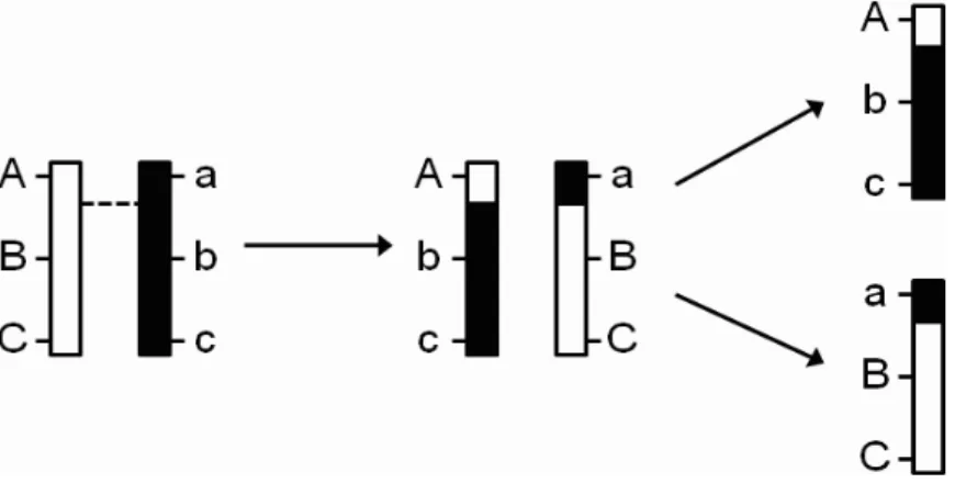
Genotypic variation is created from a process called crossing over. In crossing over, the paired chromosomes exchange segments, as shown in Figure 1.1, and produce two child chromosomes, or gametes. The result of this process is called recombination. The event in which crossing over occurs is called meiosis. Although meiosis takes place in all plant and animal sex organs, recombination can be detected only when the chromosome segments exchanged carry different alleles.

Gametogenesis occurs in both father and mother. One gamete from the father will pair with one from the mother to form the progeny chromosome pair.

(11)

1.3 Recombination fraction

There is a certain probability of crossing over between every two loci. Consider a pair of chromosomes with two loci, A and B. This pair forms a new gamete as shown in Figure 1.2. The parental chromosomes have genotypes AaBb. The genotype of the gamete is one ofAB,

ab, Ab, or aB. AB and ab are called parental types because the loci are the same as those of the parents, while Ab and aB are recombinant types. Recombinant types are the result of crossing over.

Although the true probability of crossing over is not known, it can be estimated from the proportion of recombinant types observed in a mating experiment. This proportion is called the recombination fraction, or r. Let fXY be the frequency of gamete XY. The

recombination fraction between locus A and B, or rAB in this example is then rAB =

(fAb+faB)/(fAB +fab+fAb+faB).

The smaller the recombination fraction, the lower is the probability of a crossover. When r is very small, the two loci are said to be tightly linked. When the two loci are unlinked, the genotypes of these loci are independently sampled during gametogenesis. In this case, asymptotically, the frequency of parental types and of recombinant types are the same, or r = 0.5.

For visualization of markers in a genetic map, it is convenient to cast recombination

Figure 1.1: A pair of chromosomes exchange segments via crossing over. The broken line shows the crossover point.

(12)

fractions as genetic distances. Since these fractions do not have an additive relationship,

i.e., for loci A, B, and C, rAB+rBC 6=rAC, amapping function is required to convert them

into distances to preserve additivity. With one of these functions, recombination fractions between pairs of loci can be used to construct a genetic map. In genetic maps, genetic distances are expressed in terms of Morgans (M) or centiMorgans (cM), after geneticist Thomas Hunt Morgan.

1.4 Mapping population and mating design

A mapping population for QTL analysis starts with a cross of two parents that have con-trasting values for traits of interest. These parents ideally have homozygous genotypes at all loci. In plants such parents are created by repeated self-pollination, orselfing, over multiple generations. These parents are known as inbred lines, or simply lines.

A mating design is a description of the crosses used to produce recombinant progeny starting with the inbred parents. Its goal is to create genotypic variation (arising from random parental chromosome sampling) at each locus, and recombination (arising from crossing over) between loci. The first governs the accuracy of QTL effect estimates and the second that of QTL location estimates.

Figure 1.2: The assortment of gametes produced in gametogenesis. The upper half shows the parental chromosome pair, with genotype AaBb; the lower half shows the array of gametes that it can produce. AB and ab represent parental and Ab and aB recombinant gametes.

(13)

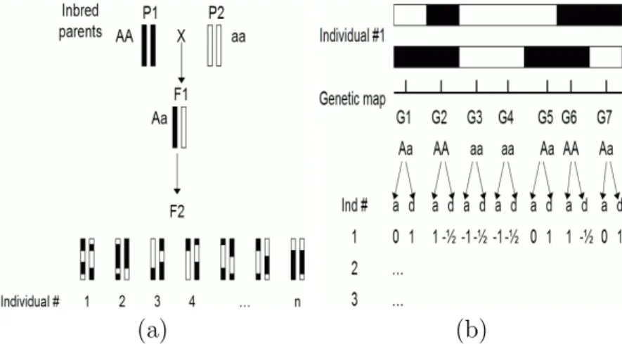
First, the inbred parents are crossed to form an F1 progeny. When both parents are all homozygous with differing alleles at every locus, the F1 progeny are all heterozygous. Then, crosses may be carried out either to self each F1 plant to form F2 progeny (Figure 1.3(a)), or to cross the F1 with one of the parents to form backcross (BC1) progeny. In the F2, there are two recombinationally informative meioses per progeny, one for each parent, while in the BC1 there is only one, in the F1 parent.

Recombinant inbred lines (RILs) are another commonly used mating design for QTL analysis, in which repeated selfings are performed over several (usually 6–8) generations from the F1. The repeated selfings yield progeny with homozygous genotypes at almost every locus. There are two recombinationally informative meioses per progeny per generation, one in each parent per progeny per generation.

Haploid doubling (DH) is also a common mating design. DH creates an instant homozy-gote through methods such as anther culture, in which the male gametes of an F1 progeny are cultured and then treated with a chemical to induce doubling. In DH, there is only one meiosis per progeny, i.e., from the F1 parent. A DH progeny, like a RIL, can be selfed to create genetically identical offspring for replicated experiments.

Each mating design produces different proportions of genotypes for each locus. These proportions are the unconditional genotypic probability of each locus. For example, in an

(a) (b)

(14)

F2 population, the expected frequency distribution ofaa, Aa, andAAgenotypes is 1:2:1. In other words, the genotypic probability distribution for all loci is 0.25, 0.5, and 0.25, for aa,

Aa, andAA, respectively. In the BC1, the ratio is 1:1:0, and in the RIL and DH, it is 1:0:1.

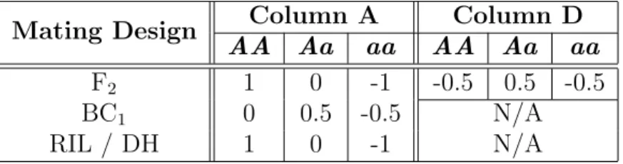
Table 1.1: Conversion table for common mating designs. The numbers in column A de-scribe a contrast, i.e., they sum to 0. The numbers in column D dede-scribe a contrast corrected for the Aa genotype because Aa and aA are indistinguishable.

Mating Design Column A Column D

AA Aa aa AA Aa aa

F2 1 0 -1 -0.5 0.5 -0.5

BC1 0 0.5 -0.5 N/A

RIL / DH 1 0 -1 N/A

1.5 Genotypic assay and conversion to numerical

val-ues

After the mapping population is formed, the genotypes of the progeny at preselected loci are assayed. The loci upon which genotypes are assayed are called DNA markers.

After the genotypes from all progeny are assayed, they are converted to numeric form according to Table 1.1 and Figure 1.3(b). The conversion is done by multiplication of the genotype data by a suitable contrast. For example, for an F2 population, the contrast in column A is used to measure an additive effect, which is the difference between the phenotypic means of the two homozygous genotypes AA and aa. The contrast in column D is used to measure a dominance effect, which is the difference between the phenotypic means of theAagenotype and the average of the homozygotes. When only two genotypes are present, such as only Aa and aa in a BC1 design, only the additive effect can be estimated. These values are used in QTL mapping as the values of the explanatory variables.

(15)

1.6 Summary of a QTL mapping process

In summary, QTL mapping is done as follows:

• Select two inbred lines that have contrasting values in traits of interest.

• Make a mapping population from these lines with a suitable mating design.

• If a genetic map is available, select a set of loci as markers that are dense enough to cover the entire map. If a genetic map is not available, there are methods to create and select markers from which a genetic map can be constructed.

• Assay the genotypes of each progeny at the selected markers.

• Assay the phenotypes or traits of interest.

(16)

Chapter 2 Review of existing QTL mapping

methods

2.1 Method overview

The statistical model used for QTL analysis is usually a general linear model (GLM), y=

Xβ +, where y represents quantitative trait data (e.g., plant height), X represents the genotypic data as described previously,β represents QTL effects, andrepresents residuals. These are usually assumed to be independent, with ∼ N(0, σ2_I

n), where In is the n×n

identity matrix, with n the number of observations. Here, y is an n×1 vector, X is an n×(cg+ 1) matrix, andβis a (cg+ 1)×1 vector, wherecis the number of effects per marker and g is the number of markers in the model. In the F2 design, c = 2 (e.g., additive and dominance effects), while in BC1 and RIL, c = 1. The number g of markers in the model varies according to the QTL-mapping method. In addition to the genotypic values, the X

matrix may contain non-genetic factors whose fixed effects are of interest. The structure of

X varies with the method.

In its simplest form (i.e., single-marker regression, or SMR), the QTL analysis uses the genotypic data of one marker at a time (g = 1). At each marker, a statistic, typically a LOD score, is computed. The LOD score is a log to base 10 of a likelihood ratio test (LRT). In this test, the null hypothesis is that the marker has neither additive nor dominance effect, while the alternative hypothesis is the negation of the null hypothesis. This process is repeated

(17)

for all m markers; that is, the model is fitted to each marker, resulting in m tests. If an association between an existing marker and the trait is detected, i.e., if the marker has a LOD score exceeding some predefined threshold, it is inferred that a QTL is located near that marker based on the observation that the genotypes of loci that are closer together are more likely to be inherited together. So to increase the odds of detection of a true QTL, and to refine the precision of location estimates, the sampled markers must be adequately densely distributed.

Multiple-testing issues and correlations among the test statistics due to linkage make it difficult to determine a statistically significant threshold for QTLs. The conventional threshold of LOD 3 based on the asymptotic distribution may not necessarily reflect the true significance threshold (Mangin et al. 1994).

The multiple-testing problem can be addressed by false discovery rate (FDR) methods (Benjamini and Hochberg 1995; Storey and Tibshirani 2003) and permutation analyses (Churchill and Doerge 1994). In FDR methods, the rate of false discovery or false positives is estimated for determining the correct cutoff (Benjamini and Yekutieli 2005). In permutation analysis, the LOD score threshold is empirically sampled under the null hypothesis. In general, permutation analysis is the preferred method because of the correlation among the statistics due to linkage.

Inferring the QTL genotype within marker intervals may improve QTL detection ac-curacy, especially when obtaining a dense map of a particular species is not possible for technical and/or economic reasons. It requires a controlled mating so that the prior proba-bility of each genotype for each marker is known. This probaproba-bility enables the inference of QTL genotypic probability at any given point within marker intervals. Such inference is use-ful in QTL interval mapping (IM). In QTL IM, each chromosome is divided into equal-sized intervals, measured in units of genetic distance.

Inference of QTL genotype (Lander and Botstein 1989) relies on the posterior proba-bility distribution of QTL genotype given the genotypes of markers flanking the QTL, the

(18)

recombination fraction between the QTL and the flanking markers, and the unconditional genotypic probability associated with the mating design. This approach is also useful for computing the genotypic probability distribution of missing marker data.

Consider a QTL Q between markers A and B, with two alleles each in the population. LetAand B denote alleles contributed by the first parent and a and b those by the second. Let dXY and rXY denote the distance and the recombination fraction between X and Y.

A mapping function (Haldane 1919) is used to convert the distance into the recombination fraction by rXY = (1−exp(−2dXY))/2, where dXY is expressed in Morgan. The expected

frequency of any gamete can be expressed in terms of recombination fractions. For example, at meiosis in the F1, the probabilities of the two nonrecombinant gametesAQB andaqb are both (1−rAQ)(1−rQB)/2 reflecting the absence of recombination between both AQ and QB. Thus, given the flanking marker genotypes AA and BB, the probability that GQ, the

genotype at QTL Q, equals QQ is

P(GQ =QQ|A=AA, B=BB) = (1−rAQ)2(1−rQB)2/4

because it is formed by pairing two AQB gametes. Likewise, the probability of Qq and qq

genotypes are P(GQ =Qq|A=AA, B=BB) = (1−rAQ)(1−rQB)rAQrQB/2 and P(GQ =qq|A=AA, B=BB) = r2AQr 2 QB/4

The preceding method is practical only for simple mating designs such as BC1 and F2. A matrix method accomodates more complex mating designs and incompletely informative marker genotypes. A Markov-chain approach (Jiang and Zeng 1997) was developed as a generalization allowing use of the information from all markers in the chromosome. The computation is as follows. Let pL

k and pRk be the probability of QTL k, given the markers

(19)

two vectors, A and B. Let qk be the unconditional genotypic probability from the mating

population. The expected frequency of each genotype of QTL k is a 3×1 vector given by

v= qk#(pLk#pRk) q0 k(p L k#p R k)

. This probability vector is then multiplied by the contrast vectors in Table

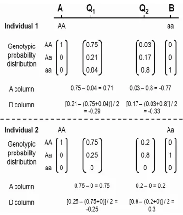
1.1, as illustrated in Figure 2.1.

The inference of QTL genotypic probability within marker intervals is required for QTL interval mapping (IM). In effect, IM interpolates the LOD score within marker intervals. The points within the intervals are treated as “virtual markers” with all-missing data. The Markov-chain approach is used to infer the QTL probability distribution, which is a 3×1 vector denoting the respective probabilities of AA, Aa, and aa genotypes.

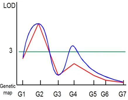
Simple interval mapping (SIM) is the IM analog of SMR. Just as in SMR, a statistic (LOD) is computed at each test position, instead of at each marker. SIM may detect a few more QTLs than SMR, as shown in Figure 2.2.

Composite interval mapping (CIM) (Zeng 1994; Jansen 1994; Jansen and Stam 1994) improves upon SIM by including in the modelbackground markers orcofactors,i.e., markers in the genetic map that are selected to reduce residual genetic variation arising from QTLs not linked to the QTL being tested. Such reduction allows more precise QTL location estimation by giving narrower peaks. Multiple interval mapping (MIM)(Kao et al. 1999) improves upon CIM by fitting multiple putative QTLs simultaneously via an EM algorithm. Bayesian interval mapping (BIM) (Satagopan et al. 1996) uses a Markov-chain Monte Carlo (MCMC) approach to sample the posterior probabilities of the QTL genotypes, effects, and locations. These are accepted with a proposal probability computed with a Metropolis-Hastings (MH) method. An improvement of BIM using reversible-jump MCMC (RJMCMC) was proposed (Sillanp¨a¨a and Arjas 1998; Stephens and Fisch 1998) to address the model-selection problem.

Only SMR, SIM, CIM, and MIM are discussed in the following subsections as pertinent to the development of multiple-trait MIM (MT-MIM) described in this report. BIM and other methods are not discussed. All derivations of formulas are available in the respective

(20)

Figure 2.1: An illustration of a Markov-chain method for inferring QTL genotype. In this example, QTL Q1 and Q2 are flanked by markers A and B. The genotypic probability

distribution (GPD) vectors of Q1 and Q2 are computed with a Markov-chain method.

In-tuitively, since Q1 is closer to marker A, its GPD should resemble marker A’s. Similarly,

since Q2 is closer to marker B, its GPD should resemble marker B’s. The value for the

cor-responding A column for the QTL is its GPD multiplied by (−1,0,1)0. Likewise, the value for the corresponding D column for the QTL is its GPD multiplied by (−0.5,0.5,−0.5)0_.

In all interval-mapping methods, these values replace the values from the substitution rule described in the text. Notice that for individual 2, the values in A and D columns for Q1

(21)

papers and are included for the purpose of MT-MIM development. MT-MIM is discussed in a separate chapter.

2.2 Least-squares-based SMR, SIM, and CIM

In single-marker regression (SMR), the number of markers in the model, g, is one and the model reduces to y=µ1+axa+dxd+. The 1vector signifies a column of ones and µis

an overall mean effect. Then×1 vectorsxaandxd are genotypic values converted as shown

in Table1.1 and Figure 1.3 (b). The scalarsaand d are the additive and dominance effects of interest to geneticists. If the mating design does not have column D in Table1.1, such as in BC1 and RIL, the term dxd is omitted, since the dominance effect cannot be estimated

for that design. The statistics are computed at each marker in turn across the genetic map. An example of an SMR plot appears in Figure 2.2.

Simple interval mapping (SIM) uses the same model used in SMR except that the values

Figure 2.2: Typical QTL-mapping profile. The single-marker regression (SMR) plot is in red. The simple interval mapping (SIM) plot is in blue. The LOD 3 line represents a significance threshold for a QTL. In this example, both SMR and SIM detect a QTL near marker G2, but only SIM can detect a QTL near marker G4.

(22)

in vectors xa and xd are computed from QTL genotype probability estimates described

previously.

In composite interval mapping (CIM), the linear model is y=µ1+axa+dxd+X∗β∗+.

The vectorsxa andxd are as in SIM.X∗ is ann×cmmatrix of background markers, where

cis the number of QTL effects (i.e., the number of columns in Table1.1for the given mating design) and m is the number of background markers. These can be selected manually or through model-selection methods, such as stepwise- or forward-selection. The entries of the

X∗ matrix are obtained by the same conversion rule used for converting marker genotypes to numbers in SMR. Thus, in the absence of background marker matrix X∗, CIM reduces to SIM.

SMR, SIM, and CIM models are simple- or multiple-regression models, which can be solved by least-squares methods. Let X = [1|xa|xd|X∗] and β0 = [µ|a|d|β∗

0

]. Thus, their models can be summarized into y=Xβ+. The solution of the QTL effects is expressed by β= (X0X)−1X0y.

Na¨ıve implementation of a least-squares method is slow and is numerically unstable owing to the finite precision of real numbers in computers. An ordinary least-squares solution involves three matrix multiplications and one matrix inversion. Precision loss occurs at every numerical operation, especially in matrix inversions. Moreover, matrix multiplications and inversions are among the most computationally expensive basic matrix operations.

To improve numerical accuracy and computation speed, QR decomposition is usually used by common statistical software. X is decomposed into Q and R, where Q is an orthogonal matrix (i.e., Q0 =Q−1) and R is an upper triangular square matrix. Thus:

β= (X0X)−1X0y= (R0Q0QR)−1R0Q0y

= (R0R)−1R0Q0y=R−1R0−1R0Q0y=R−1Q0y Rβ=Q0y

The solution forβ can be obtained by backward substitution. Numerical accuracy is im-proved because matrix inversion is no longer necessary and only two multiplications are

(23)

needed. Computation speed is improved because partial QR decomposition can be per-formed for each marker or interval. Result computation from partial decomposition is much faster than from full decomposition.

The null hypothesis is that the QTL effects are zero (a=d= 0),i.e., there is no QTL. In SMR and SIM, the null model is y=µ1+. In CIM, the null model isy=µ1+X∗β∗+. The corresponding F statistics are computed. LOD score can be obtained from LOD =

n

2 log 10log

F _dfEdfR + 1 (Doerge 1995), where n is the number of progeny, dfR and dfE are

the degrees of freedom for regression and error, and F is the F statistic.

2.3 EM-based SMR, SIM, and CIM

Single-marker regression (SMR), simple (SIM), and composite interval mapping (CIM) can also be solved by an EM algorithm, as derived in (Kao and Zeng 1997).

Assuming the CIM model and iid Normal for the error term, the joint likelihood function (Kao and Zeng 1997) for θ= (p, a, d,β, σ2) of n individuals is as follows:

L(θ|y,X) = n Y j=1 " ₃ X i=1 pjiφ yj−µji σ #

where φ(·) is a standard normal pdf, µj1 = a − d/2 + Xj∗β

∗ , µj2 = d/2 + Xj∗β ∗ , and µj3 = −a−d/2 +Xj∗β ∗

. The index i iterates over genotypes AA, Aa, and aa. Thus, µji

and pji denote the mean and the prior probability (given flanking markers) of the ith QTL

genotype.

An EM algorithm can then be used to obtain maximum-likelihood estimates (MLE) of

θ. The normal mixture of the preceding equation can be treated as an incomplete-data problem (Dempster et al. 1977) since the QTL genotypes are unknown. Let

gj(x∗j, z ∗ j) =    pj1 if x∗j = 1 andz ∗ j =− 1 2 pj2 if x∗j = 0 andz ∗ j = 1 2 pj3 if x∗j =−1 and z ∗ j =− 1 2

(24)

selected background markers, and explanatory variables Xj are treated as observed data,

denoted by y(obs,j). The conditional distribution of observed data given missing data is

yj|(θ, Xj, x∗j, z ∗ j)∼N(x ∗ ja+z ∗ jd+Xjβ, σ2)

Thus, the density of the complete-data, y(com,j), is

f(y(com,j)|θ) = f(y(obs,j)|θ, Xj, x∗j, z

∗ j)g(x ∗ j, z ∗ j)

The E step of the EM algorithm is as follows.

Qθ|θ(t)= Z

logL(θ|ycom)f(q∗|yobs,θ =θ(t))dq∗

= Z log " _n Y j=1 φ yj−µj σ gj(x∗j, z ∗ j) # ×f(q∗|yobs,θ =θ(t))dq∗

By Fubini’s theorem (Fubini 1958):

Q θ|θ(t) = n X j=1 Z log φ yj−µj σ gj(x∗j, z ∗ j) ×f(q_j∗|y(obs,j),θ =θ(t))dqj∗ = n X j=1 3 X i=1 log φ yj−µj σ pji × pjiφ yj−µ(t)ji σ(t) 3 X k=1 pjkφ yj −µ(_jkt) σ(t) ! = n X j=1 3 X i=1 log φ yj−µj σ pji ×π_ji(t)

Observe that by Bayes’ ruleπji is the posterior probability of the QTL genotype. Assuming

that the true QTL genotype is the ith _{genotype, write}

fq∗_j|y(obs,j),θ =θ(t) = fy(obs,j)|q∗j,θ =θ (t) fq_j∗|θ=θ(t) fy(obs,j)|θ=θ(t) = φ yj−µ(t)_ji σ(t) pji 3 X k=1 pjkφ yj−µ (t) jk σ(t) ! =πji

(25)

In the M step, the MLE solution is obtained by differentiation of Qθ|θ(t) with respect to θ, yielding a(t+1) = n X j=1 π_j(t₁)−π_j(t₃) yj−Xjβ(t) −1 2 π(_jt₃)−π_j(t₁) d(t) n X j=1 π_j(t₁)+π(_jt₃) = y−Xβ(t) 0 Π(t)_d 1−10Π(t)(d1#d2)d(t) 10_Π(t)₍_d 1#d1) d(t+1) = n X j=1 1 2 h −π_j(t₁)+π_j(t₂)−π(_jt₃) yj −Xjβ(t) −π_j(t₃)−π_j(t₁)a(t)i n X j=1 π_j(t₁)+π(_j₂t)+π_j(t₃) = y−Xβ(t) 0 Π(t)d2−10Π(t)(d1#d2)a(t) 10_Π(t)₍_d_2#_d₂₎

where # denotes the Hadamard (componentwise) product of two vectors, Π = {πji}n×3,

d1 = (1,0,−1)0, and d2 = (−₂1,1₂,−1₂)0.

Let e(t)= (a(t), d(t))0. The equations above simplify to

e(t+1)=r(t)−M(t)e(t) where r(t) =   (y−Xβ(t))0Π(t)d1 10_Π(t)₍_d 1#d1) (y−Xβ(t)₎0_Π(t)_d 2 10_Π(t)₍_d 2#d2)   and M(t) = " 0 1₁00Π_Π(t)(t)(₍d_d_1#1#_dd2)₁₎ 10Π(t)₍_d_2#_d₁₎ 10_Π(t)₍_d_2#_d₂₎ 0 # β(t+1) = (X0X)−1X0y−Π(t)De(t+1) σ2(t+1) = 1 n y−Xβ(t+1) 0 y−Xβ(t+1)−y−Xβ(t+1) 0 Π(t)De(t+1) +e0(t+1)V(t)e(t+1) where D= (d1,d2) and V(t) = 10Π(t)(d1#d1) 10Π(t)(d1#d2)

(26)

Note that V, but not M, is symmetric.

In the first iteration, Π is filled with the genotypic distribution obtained from the Markov-chain approach described previously. The vectors β and e are filled with the esti-mates from the least-squares method.

The estimates of the parameters and the Π matrix are updated as described until con-vergence. The null hypothesis is a = d = 0 and the log likelihood for the null hypothesis is also computed. A likelihood ratio score (LR) is computed and LOD score is obtained by LOD = LR/(2 log 10).

2.4 Multiple interval mapping (MIM)

MIM (Kao et al. 1999) builds upon the EM solution of composite interval mapping (CIM). Instead of fitting background markers, it fits q QTLs simultaneously. Thus, the index i in the EM solution above runs from 1 to 3q _{(or 2}q _{in the absence of a dominance effect),}

accounting for all possible QTL genotype combinations. The joint likelihood function now becomes: L(θ|y,X) = n Y j=1 " ₃q X i=1 pjiφ yj−µji σ #

The updating rule for the posterior probability of QTL genotype becomes:

π_ji(t+1) = φ yj−µ(t)_ji σ(t) pji 3q X k=1 pjkφ yj −µ (t) jk σ(t) ! ∀i∈ {1, . . . ,3 q_}

The genetic design matrixD3q_×₂ =1_q⊗ {d₁,d₂}, if both additive and dominance effects are present, or D3q_×₁ =1_q⊗ {d₁}, if only an additive effect is present. The symbol ⊗ denotes the Kronecker product.

Consequently:

(27)

r =      y−Xβ(t) 0 Π(t)_d 1 10_Π₍_D i#Di)      e×1 M= 10Π(t)₍_d i#dj) 10_Π(t)₍_d i#di) e×e

where e is the number of columns of D.

The formulas above are a straightforward extension to allow estimation of both dom-inance effect and non-genetic factors. The original paper describes only the formulas for designs with only additive effect present and no non-genetic factors. Here, matrix X con-tains only non-genetic factors, while the other matrices and vectors are kept the same as those of CIM. If there are no non-genetic factors, then X=1.

Since fitting too many QTL at once is computationally expensive, MIM uses a stepwise or “chunkwise” selection method to add QTLs into the model. In stepwise selection, QTL is added to the model one by one. In chunkwise selection, several QTLs are added to the model at a time. The QTL selection proceeds just like usual model-selection procedures.

2.5 Multiple-trait composite interval mapping

(MT-CIM)

Multiple-trait QTL analysis is QTL analysis applied to several traits simultaneously. Such analysis was shown (Jiang and Zeng 1995) to improve the statistical power of QTL detec-tion test and the precision of parameter estimadetec-tion by taking into account the correladetec-tion structure among the traits. In addition, such analysis provides formal procedures to test for pleiotropy, i.e., whether a QTL affects all selected traits, and QTL-by-environment (Q×E) interaction.

Multiple-trait CIM (Jiang and Zeng 1995) builds upon the EM solution of single-trait CIM. The model is the same as that of CIM, except that all matrices and vectors are expanded to t variates. If t denotes the number of traits (i.e., variates), the model is expressed by Y n×t = x n×11a×t+nz×11d×t + X n×(2k+p+1)(2k+Bp+1)×t + E n×t

(28)

where k is the number of cofactor markers (with two effects calculated per marker) and p is the number of non-genetic covariates. Notice that if t = 1, this model reduces to CIM’s model.

Although the encoding of QTL genotypes is different, the steps to derive the solution are essentially the same. In the original paper, xj takes values of 2, 1, and zero for respective

QTL genotypes AA, Aa, and aa. zj takes value 1 if the QTL genotype is Aa, otherwise 0.

The joint likelihood function of the data is

L1 =

n

Y

j=1

[p2jφ2(yj) +pijφ1(yj) +p0jφ0(yj)]

where the pij are the prior probability of QTL genotypes of AA, Aa, and aa and φi(·) is

multivariate normal with variance σ and mean uj2 = XjB+ 2a, uj1 =XjB+a+d, and uj0 =XjB, respectively.

The log-likelihood function is given by

ln(L1) = k∗− n 2 ln ˆ V + n X j=1 ln p2jexp 1 2[yj−2â−XjBˆ]Vˆ −1_[_y j −2â−XjBˆ]0 +p1jexp 1 2[yj −â− ˆ d−XjBˆ]Vˆ−1[yj−â−dˆ−XjBˆ]0 +p0jexp 1 2[yj −XjBˆ]Vˆ −1_[_y j−XjBˆ]0 =k∗−n 2 ln ˆ V − 1 2 n X j=1 [yj −XjBˆ]Vˆ−1[yj−XjBˆ]0 + n X j=1 ln p2jexp[2â ˆV−1[yj −â−XjBˆ]0] +p1jexp[(â+dˆ)Vˆ−1[yj − 1 2â− 1 2 ˆ d−XjBˆ]0] +p0j

(29)

Differentiating the log-likelihood function with respect to its parameters yields a(t+1) = q 0₍_t₊₁₎ 2 2q0₂(t+1)1(Y−XB (t)₎ d(t+1) = " q0₁(t+1) q0₁(t+1)1 − q0₂(t+1) 2q0₂(t+1)1 # (Y−XB(t)) B(t+1) = (X0X)−1X0[Y−(2q(₂t+1)+q(₁t+1))a(t+1)−q(₁t+1)d(t+1)] V(t+1) = 1 n h (Y−XB(t+1))0(Y−XB(t+1))−4(q0₂(t+1)1)a0(t+1)a(t+1) −(q0₁(t+1)1)(a(t+1)+d(t+1))0(a(t+1)+d(t+1)) i

whereq(₂t+1) andq₁(t+1) are the respectiven×1 vectors ofq₂(t_j+1)andq₁(t_j+1), and fori= 0,1,2,

qij = pijφ(it)(yj) 2 X k=0 pkjφ(_kt)(yj)

There are several modes of hypothesis testing in multiple-trait analysis:

1. Joint QTL mapping Is there any QTL detected for any trait?

Under joint-mapping the hypotheses to be tested are H0 : a = d = 0 vs. HA :

otherwise. In this case, the log-likelihood under H0 is given by

ln(L0) = ln " _n Y j=1 φ0(yj) # =k− n 2 ln| ˆ V0| −nm/2

where V0ˆ = (Y−XB0)0(Y−XB0)/n and B0 = (X0X)−1X0Y. The LOD score is obtained from LOD =− 1

ln(10)ln L0 L1 .

2. Test of pleiotropic effects Is there any QTL that affects all traits?

The hypotheses to be tested are H0 :ai = 0 or di = 0 for some trait i vs. HA :a6= 0

and d6= 0 (i.e., testing if the QTL effects are zero in at least one trait). In this case, there are multiple null hypotheses. The log-likelihood ratio score can be obtained from the formulas derived above, with the appropriate effects set to zero. Although

(30)

score, it is usually taken as the minimum of the LOD scores at a particular marker or interval.

3. Test of close linkage versus pleiotropy Is the detected pleiotropic QTL not an artefact of several closely-linked QTLs?

A QTL that affects all traits is not necessarily a pleiotropic QTL. It may be an artefact of several closely linked QTLs. This test is designed to distinguish the two, especially if the pleiotropic LOD score peak is wide.

Let pos(i) be the position of the currently tested QTL for trait i. The hypotheses to be tested are H0 : pos(i) = pos(j), ∀i, j ∈ {1, . . . , t} vs. HA : otherwise. In this case,

the position of QTL at trait iis shifted a little bit (1–2 cM) to either side and tested with the QTL at trait j. A LOD score is then computed in similar manner. If H0 is rejected, then the QTL involved is not a pleiotropic QTL.

4. QTL by environment (Q×E) analysis Does the QTL affect one trait differently from the others?

This test is particularly useful when the traits being tested are the same trait (e.g., grain yield) in the same set of individuals (e.g., replicated lines) but measured in different environments.

Let ai and di be the additive and dominance effect of a given QTL for a given trait.

The hypothesis to be tested is

H0 : (ai =aj =a) and (di =dj =d), ∀i, j ∈ {1, . . . , t}

vs. HA: not H0.

(31)

replaced by a and d. In the CM step a(t+1) = q 0₍_t₊₁₎ 2 2c(t)_q0(t+1) 2 1 (Y−XB(t))(V(t))−11 d(t+1) = " q0₁(t+1) c(t)_q0(t+1) 1 1 − q 0₍_t₊₁₎ 2 2c(t)_q0(t+1) 2 1 # (Y−XB(t))(V(t))−11 where c(t)₌₁0_V(t)₁_.

So, under H0, the log-likelihood now becomes:

ln(L0) =k∗− n 2ln| ˆ V| − 1 2 n X j=1 (yj−xjBˆ)Vˆ−1(yj−xjBˆ)0 + n X j=1 lnhp2jexp[(2a)10Vˆ−1(yj−10a−xjBˆ)0] +p1jexp[(a+d)10Vˆ−1(yj−10(a+d)/2−xjBˆ)] +p0j i

The LOD score is obtained as LOD =− 1 ln(10)ln L0 L1 .

2.6 Summary

Single-marker regression (SMR), and simple (SIM), composite (CIM) and multiple interval mapping (MIM) can be solved using the same general linear model framework. SMR and SIM use essentially the same model to detect QTL: the former uses marker data, while the latter uses interpolated QTL genotype estimates. CIM and MIM also use the same model. CIM uses marker data, while MIM uses the calculated QTL estimates as the background.

Multiple-trait CIM (MT-CIM) extends CIM for correlated traits (Jiang and Zeng 1995). MT-CIM exploits the correlation structure to improve the accuracy of QTL detection. In addition, it provides additional tests that cannot be performed for single traits, such as pleiotropy and QTL-by-environment interaction.

In the absence of multiple traits, MT-CIM reduces to single-trait CIM and its perfor-mance and accuracy are the same as that of CIM. Multiple-trait analyses, such as pleiotropy

(32)

Although SIM and CIM are still widely used today, they have less power than, and have been largely superseded by, MIM (Kao et al. 1999). SIM and CIM may be useful for preliminary analyses because they can be computed rapidly. Although MIM computation is much slower than that of SMR, SIM, or CIM, modern computers can perform MIM computation in seconds to minutes.

Since MT-CIM improves upon CIM, multiple-trait extension of MIM (MT-MIM) should also improve upon MIM. Since MIM has been shown (Kao et al. 1999) to give narrower peaks for QTLs than CIM, MT-MIM is expected to be more precise than MT-CIM. This motivates the development of MT-MIM.

(33)

Chapter 3 Multiple-trait multiple interval

mapping (MT-MIM)

3.1 Derivation

The MT-MIM solution is based on single-trait MIM (MIM) using the models of multiple-trait CIM. The model is as follows:

Y n×t= q X i=1 xi n×1 ai 1×t + zi n×1 di 1×t + X n×(p+1) B (p+1)×t + E n×t

where q is the number of QTLs being fitted simultaneously, t is the number of analyzed traits, p is the number of non-genetic fixed factors, and E is random error, iid Normal(0,

Σ).

The differences between MT-MIM and single-trait MIM or MT-CIM are as follows. Here,

Y is a matrix, similar to that of MT-CIM, instead of a vector as in MIM. Instead of testing one QTL at a time in MT-CIM, the model tests q QTLs at a time, as in MIM. The reader will notice that the method development is very similar to that of MIM (Kao et al. 1999).

Using the same framework, the joint likelihood for the parameter θ = (p,a,d,B,Σ) is

L1 =L(θ|Y,X) = n Y j=1 " ₃q X i=1 pjif(yj;µji,Σ) #

(34)

The E step of the EM algorithm is very similar to that of MT-CIM, except now the pdf used in the derivation is multivariate instead of univariate normal.

Q θ|θ(t) = Z

logL(θ|Ycom)f(Q∗|Yobs,θ=θ(t))dQ∗

= Z log " _n Y j=1 f(yj;µji,Σ)gj(x∗j, z ∗ j) # ×f(Q∗|Yobs,θ=θ(t))dQ∗

By Fubini’s theorem (Fubini 1958):

Qθ|θ(t)= n X j=1 Z logf(yj;µji,Σ)gj(x∗j, z ∗ j) ×f(q∗_j|y(obs,j),θ =θ(t))dq∗j = n X j=1 3q X i=1 log [f(yj;µji,Σ)pji]× pjif(yj;µji,Σ) 3q X k=1 pjkf(yj;µji,Σ) = n X j=1 3q X i=1 log [f(yj;µji,Σ)pji]×π (t) ji

Note that the summation on index i is now from 1 to 3q, as in MIM, instead of 3 as in MT-CIM.

Thus, the updating rule for the posterior probability of the QTL genotype becomes:

π_ji(t+1) = f(yj;µji,Σ)pji 3q X k=1 pjkf(yj;µji,Σ) ∀i∈ {1, . . . ,3q}

Note that the posterior probabilities of the q QTLs are updated at the same time using a multivariate instead of a univariate normal pdf.

Differentiate Q

θ|θ(t)

with respect to each parameter to yield

E(t+1)=r(t)−M(t)E(t) where r(t) =   (Y−Xβ(t)₎0_Π(t)_d 1 10_Π(t)₍_d 1#d1) (Y−Xβ(t))0Π(t)_d 2 10_Π(t)₍_d _#_d ₎   and M(t) = " 0 1₁00Π_Π(t)(t)(₍d_d_1#1#_dd2)₁₎ 10Π(t)(d2#d1) 10_Π(t)₍_d 2#d2) 0 #

(35)

Note that E is a eq×t matrix of effects (not of residuals), where e is the number of effects as defined in the previous chapter.

B(t+1) = (X0X)−1X0Y−Π(t)DE(t+1) Σ(t+1) = 1 n Y−Xβ(t+1)−Π(t)DE(t+1) 0 Y−Xβ(t+1)−Π(t)DE(t+1)

where D= (d1,d2), as defined in previous sections.

MT-MIM can be considered as a generalization of both MIM and MT-CIM. If t = 1, MT-MIM reduces to MIM, while q = 1, MT-MIM reduces to MT-CIM.

The hypothesis testing is very similar to that of multiple-trait CIM:

1. Joint QTL mapping Is there any QTL detected for any trait?

Under joint-mapping the hypotheses to be tested areH0 :E= 0 vs. HAotherwise. In

this case, the log-likelihood under H0 is given by

ln(L0) = ln " _n Y j=1 f(yj;µj,Σ) # =k−n 2 ln| ˆ V0| −nm/2

where V0ˆ = (Y−XB0)0(Y−XB0)/n and B0 = (X0X)−1X0Y. The LOD score is obtained from LOD =− 1

ln(10)ln L0 L1 .

2. Test of pleiotropic effects Is there any QTL that affects all traits?

The hypotheses to be tested are HA : E 6= 0 vs. H0 otherwise (i.e., the effects of at least one QTL are zero in at least one trait). In this case, there are multiple null hypotheses. The log-likelihood ratio score can be obtained from the formulas derived above, with the appropriate effects set to zero. The combined LOD score is defined as the minimum of the LOD scores at a particular interval.

3. QTL by environment (Q×E) analysis Does the QTL affect one trait differently from the others?

(36)

This test is useful when the traits being tested are the same trait (e.g. grain yield) in the same set of individuals (e.g., replicated lines) but measured in different environ-ments.

Letai and di be the additive and dominance effects of a given QTL for a given trait.

The hypothesis to be tested is

H0 :ai =aj =aand di =dj =d, ∀i, j ∈ {1, . . . , t} vs. HA: not H0. a(t+1) =10_t(Σ(t))−1    Y−Xβ(t) 0 Π(t)_d 1−(10t⊗1n)0Π(t)(d1#d2)d(t) c(t)₁0_Π(t)₍_d 1#d1)    d(t+1) =10_t(Σ(t))−1    Y−Xβ(t) 0 Π(t)_d 2−(10t⊗1n)0Π(t)(d1#d2)a(t) c(t)₁0_Π(t)₍_d 2#d2)    where c(t) ₌₁0

tΣ(t)1t and 1t is a t×1 column vector of ones.

So, underH0, the log-likelihood is obtained by substitution ofaanddintoL1formula. The LOD score is obtained similarly.

Although the original MIM may use either stepwise or chunkwise selection (Kao et al. 1999) to add QTLs into the model, my implementation uses stepwise selection. This is because it saves computation time while generally yielding the same model as the chunkwise method.

3.2 Implementation details

In general, MIM produces sharper peaks than CIM. Multiple-trait MIM (MT-MIM) is ex-pected to behave similarly relative to MT-CIM. Since MIM produces sharper peaks than

(37)

CIM, the test of close linkage versus pleiotropy in MT-CIM is not useful in practice. For this reason, the implementation of this test is omitted in this thesis.

MT-CIM treats the variance–covariance matrix of the trait data as unstructured, which effectively limits the number of traitst because the number of estimated parameters in the matrix is t(t+1)₂ . The MT-MIM method will also treat the matrix as unstructured, and hence, is subject to the same limitation.

Although the models used in the previously explained methods fall within the general linear model (GLM) framework, common statistical software does not necessarily provide solutions to all of them. SMR, SIM, and CIM models are merely simple or multiple regres-sion, which can be solved by SAS or R. However, in MIM, a slight modification in the EM algorithm to accommodate QTL genotypic probabilities makes it necessary to move beyond standard linear-models packages.

Although the authors of MIM and multivariate CIM have published their software on-line, there are problems to using or extending them, prompting the need to develop custom software. The two programs are written in different languages: MIM in FORTRAN, mul-tivariate CIM in C. In addition, their implementations are restricted to very few mating designs (only backcross and F2), limiting their use and adoption by general analysts who are usually unfamiliar with programming and statistics.

QGene 4 (Joehanes and Nelson 2008), written in the Java language for multi-platform operation, accommodates rapid QTL-analysis method implementation with a plug-in ar-chitecture allowing component reusability. QGene 4 was a complete rewrite of an earlier application (Nelson 1997), which implemented only SMR and SIM. Current QGene 4 has CIM, MIM, and multiple-trait CIM implemented.

MT-MIM is built in QGene as a plug-in so that it can reuse many QGene components and hence shorten the development time. Moreover, QGene has a simulation module that can be used to compare the accuracy of MT-MIM and other methods.

(38)

Chapter 4 Results of QTL analysis using

MT-MIM

4.1 Description of the dataset and previous results

The data used in this experiment were derived from a cross between barley cultivars Steptoe and Morex (Kleinhofs et al. 1993), and contain grain yield data measured for 150 DH lines grown in 16 different environments (yld01–yld16). While there are no missing trait data, some genotype data are missing.

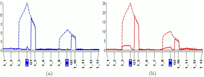
It is known that a QTL on chromosome 3 influences grain yield (Hayes et al. 1994). A plot of chromosome 3 shows profiles for simple (SIM), composite (CIM), and multiple interval mapping (MIM) is presented in Figure4.1a and b. CIM gives narrower peaks than SIM. These figures confirm that CIM is more precise than SIM and MIM is more precise than CIM.

4.2 Results of MT-MIM on barley data

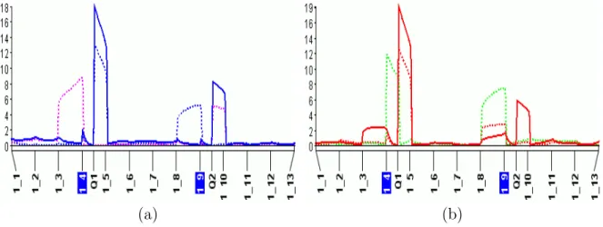
The preliminary results of MT-MIM applied to the first three traits (yld01–yld03) of the Steptoe × Morex barley data were promising. Not only does MT-MIM show a larger LOD score, MT-MIM also manages to “merge” disparate QTL locations on chromosome 3 as shown in Figure 4.2. Single-trait analysis typically cannot consolidate disparate QTL positions.

(39)

(a) (b)

Figure 4.1: (a) CIM improves upon SIM by giving narrower peaks. Broken line: SIM, solid line: CIM; (b) MIM improves upon CIM by giving even narrower peaks. Broken line: CIM, solid line: MIM. Highlighted markers represent cofactors selected for CIM. Vertical axis represents LOD score. Horizontal axis represents genetic location on the chromosome.

(a) (b)

Figure 4.2: (a) Single-trait MIM on traits yld01–yld03 gives different QTL location esti-mates in chromosome 3; (b) MT-MIM consolidates QTL locations and shows higher LOD scores. The QTL on chromosome 3 influences at least one of the three traits. Vertical axis represents LOD score. Horizontal axis represents genetic location on the chromosome.

(40)

The QTL in chromosome 3 is known to be pleiotropic and to act differently in different locations. MT-MIM is able to detect it, as shown in Figure 4.3.

(a) (b)

Figure 4.3: (a) QTL on chromosome 3 is shown to be pleiotropic for traits yld01–yld03. This QTL influences all three traits.; (b) Q×E analysis of yld01–yld03. The QTL between markers ABG399 andBCD828 is seen to act differently in the three different environments. The QTL between markers ABG377 andMWG555B affects only trait yld01. The Q×E test correctly shows that the QTL acts differently in different environments. The regions on the left and right of the plot also show differences in different environments although show no QTLs. Vertical axis represents LOD score. Horizontal axis represents genetic location on the chromosome.

4.3 Simulation setup and results

One hundred simulated datasets of 200 progeny each were generated by QGene for two cor-related traits in the F2 mating design. Theheritability, or the proportion of the phenotypic variance accounted for by genotypic variance, was set to 0.5. The trait correlations were chosen to be 0.9, 0.4, and 0.0, so that there were 300 datasets in total. For each trait there were two QTLs in the model, Q1 at 35 centiMorgans (cM) and Q2 at 85 cM, with the effects described in Table 4.1. The QTLs were placed on a 120-cM chromosome, with markers at 10-cM intervals. Scan interval was set to 1 cM. A QTL was declared if there was a LOD score of at least 2.8 within 15 cM of the true QTL position.

In the presence of correlation, multiple-trait CIM (MT-CIM) produced a wider peak than multiple-trait MIM (MT-MIM) in all datasets. A typical example is shown in Figure

(41)

4.4. Both methods detected all QTLs in the data 97% of datasets.

(a) (b)

Figure 4.4: Comparison between MT-MIM (solid line) and MT-CIM (broken line) when the correlation between the two traits is (a) ρ = 0.4; (b) ρ = 0.9. Highlighted markers represent cofactors selected for MT-CIM. Vertical axis represents LOD score. Horizontal axis represents genetic location on the chromosome.

In the absence of correlation, MT-CIM produced sharper peaks than those in the presence of correlation, but MT-MIM produced even sharper peaks, as shown in Figure 4.5. Both methods could detect all QTLs in the data.

QTLs detected by single-trait MIM tended to differ for each trait, regardless of the presence of correlation. A typical example is shown in Figures 4.6and4.7. Although single-trait MIM tended to either narrowly miss the QTL (25% of all cases) or completely fail to detect weaker QTL Q2 (30.4% of all cases), MT-MIM could detect all QTLs correctly.

In all cases, MT-CIM produced higher and wider peaks than MT-MIM, even after co-factors next to the QTLs were selected. Although the peaks produced by MT-MIM show lower LOD scores, they passed the permutation analysis thresholds. The average

signifi-Table 4.1: QTL effect values from comparative simulation study of MT-MIM

Trait Q1 effect Q2 effect

Additive Dominance Additive Dominance

Trait 1 1.0 0.0 0.3 0.0

(42)

Figure 4.5: Comparison between MT-MIM (solid line) and MT-CIM (broken line) when there is no correlation between the traits. Highlighted markers represent cofactors selected for MT-CIM. Vertical axis represents LOD score. Horizontal axis represents genetic location on the chromosome.

(a) (b)

Figure 4.6: Comparison between MT-MIM (solid line) and single-trait MIM (broken line) for two traits with correlation (a) ρ = 0.4; (b) ρ = 0.9 and controlled by the same two QTLs. Blue and red lines: trait 1; magenta and green lines: trait 2. These figures show that single-trait MIM may give inconsistent QTL location estimates. Vertical axis represents LOD score. Horizontal axis represents genetic location on the chromosome.

(43)

cance thresholds for MT-MIM of all datasets were 3.70 and 4.59, for α= 0.05 and 0.01. For MT-CIM, they were 3.31 and 4.3.

In single-trait MIM, the low LOD score at QTL Q2 failed to pass the significance thresh-old. For single-trait MIM, the average significance thresholds were 2.66 and 3.48.

For comparison, single-trait Bayesian interval mapping (BIM) was run on one of the datasets, as shown in Figure 4.8(a). The result suggests that unlike single-trait MIM, BIM does not suffer from QTL location-estimate disagreements. However, BIM requires much longer computation time than MIM. In addition, the computation of the QTL significance threshold using permutation takes a prohibitively long time. One 1,000-iteration permuta-tion run may take 3 to 4 hours on a dual-core Intel Core 2 Duo T9300, 2.5GHz laptop, with parallel algorithms enabled.

Simple interval mapping (SIM) performed very poorly, as expected. SIM produced a very wide peak and failed to distinguish QTLs Q1 and Q2, as shown in Figure4.8(b).

The simulation results are summarized in Table 4.2.

Figure 4.7: Comparison between MT-MIM (solid line) and single-trait MIM (broken line) for two uncorrelated traits controlled by the same two QTLs. Black broken line: trait 1; brown broken line: trait 2. This figure shows that single-trait MIM may give inconsistent QTL location estimates for two traits controlled by the same QTLs even when they are uncorrelated. Vertical axis represents LOD score. Horizontal axis represents genetic location

(44)

(a) (b)

Figure 4.8: (a) Single-trait Bayesian interval mapping (BIM) shows consistent QTL lo-cation estimates for two traits controlled by the same QTLs. (b) Simple interval mapping (SIM) fails to distinguish the two QTLs. Red line: trait 1; green line: trait 2. Vertical axis: for BIM, QTL posterior probability; for SIM, LOD score. Horizontal axis represents genetic location on the chromosome.

Table 4.2: Comparative QTL-detection accuracy of three QTL analysis methods for two traits controlled by the same QTLs, from simulation. Entries denote the percentage of the corresponding QTLs detected by the methods.

Method ρ= 0.0 ρ= 0.4 ρ= 0.9 Q1 Q2 Q1 Q2 Q1 Q2 MT-CIM 1.000 0.968 1.000 0.971 1.000 0.978 MIM (trait 1) 1.000 0.425 1.000 0.435 1.000 0.396 MIM (trait 2) 1.000 0.977 1.000 0.966 1.000 0.976 MT-MIM 1.000 0.977 1.000 0.973 1.000 0.982

(45)

Chapter 5 Discussion and conclusion

In the simulation study presented in the preceding chapter, it was shown that when the traits were governed by a set of common QTLs, single-trait analyses sometimes failed to agree on the QTL location estimates. Multiple-trait methods tended to merge the disparate QTL location estimates, even in the absence of trait correlation.

The study also showed that MT-MIM improves upon MT-CIM by giving narrower QTL peaks. Narrow peaks mean a smaller space for subsequent experimental searches for the QTL.

Why can multiple-trait analyses merge the disparate peaks given by single-trait analyses? To simplify the argument, consider a bivariate regression setting with only additive effects, with a putative QTL k. Let y1 and y2 be the trait values and xk be the encoded genotype

of QTL k. Let bk = (bk1, bk2) be the regression coefficients of y1 and y2 onxk. Let σ2i and

ρ be the residual variance for trait i and the residual correlation coefficient. Letσ_x2_k be the variance of xk. Letβi =bkiσxk/σi. (Jiang and Zeng 1995) showed in their Appendix A that the likelihood ratio test statistic for the joint analysis (LRjoint) is expected to be:

LRjoint =nln 1 + β 2 1 +β22−2ρβ1β2 1−ρ2 'nβ 2 1 +β22−2ρβ1β2 1−ρ2 , if β 2 1, β 2 2 1.

(46)

detected on the trait with lower residual variance will dominate and “unify” the effect and location of QTLs on the other traits, even if ρ = 0. Let It be a t×t identity matrix and V be the variance–covariance matrix. Since L0 ∝ |V+σk2b

0

kbk|−n/2 and L1 ∝ |V|−n/2, the general formula of expected LRjoint is:

LRjoint =−2 ln(L0/L1) =nln |V+σ_k2b0_kbk| |V| =nlnIt+σ2kb 0 kbkV−1

In this formulation, V−1 _{serves as the weight matrix that aggregates the effects of the} QTL across traits. Even if there is no correlation among the traits, i.e., V is diagonal, the effects of other traits will still influence LRjoint because the term b0kbkwill never be diagonal

if there are at least two traits influenced by the same QTL. In this case, the QTL effect on the trait with lower residual variance will prevail. This argument is also applicable for cases of multiple markers and dominance effect. The derivation is similar to the one presented in (Jiang and Zeng 1995).

Although MT-MIM takes more computation time, it was still computed very rapidly in the simulation study. The computation time depends on the number of chromosomes, chromosome length, scan interval, number of observations, and number of traits analyzed at once. For six traits and 12 chromosomes of about 200 cM, MT-CIM may take a minute or two in modern computers.

Both MT-CIM and MT-MIM treat the variance–covariance matrix as unstructured, which effectively limits the number of traits t because the number of estimated parameters in the matrix is t(t+1)₂ . The more traits included in the model, the closer the variance– covariance matrix approaches to singularity. Without having investigated the upper limit on the number of traits that should be included for a given number n of progeny, I suggest that it should not exceed d1

2 √

(47)

x. Other analyses such as mixed linear models must be used for higher numbers of traits, as adding the number of observations required for reliable estimates becomes impractical.

Despite some limitations, MT-MIM shows potential as an emerging multiple-trait QTL analysis method. It combines the accuracy of MIM and the sensitivity of multiple-trait analysis with reasonable computation time. Further investigation could involve a more ex-tensive simulation study to investigate more of MT-MIM’s properties, especially in different mating designs, in the presence of dominance effects, and in cases of linked QTLs.

(48)

Bibliography

Benjamini, Y. and Hochberg, Y. (1995), “Controlling the false discovery rate: a practical and powerful approach to multiple testing,” Journal of the Royal Statistical Society B, 57, 289–300.

Benjamini, Y. and Yekutieli, D. (2005), “Quantitative trait loci analysis using false discovery rate,”Genetics, 171, 783–790.

Churchill, G. A. and Doerge, R. W. (1994), “Empirical threshold values for quantitative trait mapping,” Genetics, 138, 963–971.

Dempster, A. P., Laird, N. M., and Rubin, D. B. (1977), “Maximum likelihood from in-complete data via the EM algorithm,” Journal of the Royal Statistical Society B, 39, 1–38.

Doerge, R. W. (1995), “The relationship between the LOD score and the analysis of vari-ance F-statistic when detecting QTL using single markers. Appendix 1: locating genes associated with root morphology and drought avoidance in rice via linkage to molecular markers,” Theoretical and Applied Genetics, 90, 969–981.

Fubini, G. (1958), “Sugli integrali multipli,” Cremonese, 2, 243–249.

Haldane, J. B. S. (1919), “The combination of linkage values, and the calculation of distances between the loci of linked factors,” Journal of Genetics, 8, 299–309.

Hayes, P., Liu, B., Knapp, S., Chen, F., Jones, B., Blake, T., Franckowiak, J., Rasmus-son, D., Sorrels, M., Ullrich, S., Wesenberg, D., and Kleinhofs, A. (1994), “Quantitative trait locus effects and environmental interaction in a sample of North American barley germplasm,”Theoretical and Applied Genetics, 87, 392–401.

(49)

Jansen, R. C. (1994), “Controlling the type I and type II errors in mapping quantitative trait loci,” Genetics, 138, 871–881.

Jansen, R. C. and Stam, P. (1994), “High resolution of quantitative traits into multiple loci via interval mapping,” Genetics, 136, 1447–1455.

Jiang, C. and Zeng, Z.-B. (1995), “Multiple trait analysis of genetic mapping for quantitative trait loci,” Genetics, 140, 1111–1127.

Jiang, C. and Zeng, Z. B. (1997), “Mapping quantitative trait loci with dominant and missing markers in various crosses from two inbred lines,” Genetica, 101, 47–58.

Joehanes, R. and Nelson, J. C. (2008), “QGene 4.0, an extensible Java QTL-analysis plat-form,” Bioinformatics, 24, 2788–2789.

Kao, C.-H. and Zeng, Z.-B. (1997), “General formulas for obtaining the MLEs and the asymptotic variance–covariance matrix in mapping quantitative trait loci when using the EM algorithm,”Biometrics, 53, 653–665.

Kao, C.-H., Zeng, Z.-B., and Teasdale, R. D. (1999), “Multiple trait mapping for quantita-tive trait loci,”Genetics, 152, 1203–1216.

Kleinhofs, A., Kilian, A., Maroof, M. S., Biyashev, R., Hayes, P., Chen, F., Lapitan, N., Fenwick, A., Blake, T., Kanazin, V., Ananiev, E., Dahleen, L., Kudrna, D., Bollinger, J., Knapp, S., Liu, B., Sorrells, M., Heun, M., Franckowiak, J., Hoffman, D., Skadsen, R., and Steffenson, B. (1993), “A molecular, isozyme, and morphological map of the barley (Hordeum vulgare) genome,” Theoretical and Applied Genetics, 86, 705–712.

Lander, E. S. and Botstein, D. (1989), “Mapping Mendelian factors underlying quantitative traits using RFLP linkage maps,”Genetics, 121, 185–199.

(50)

Nelson, J. C. (1997), “QGENE: software for marker-based genomic analysis and breeding,”

Molecular Breeding, 3, 239–245.

Satagopan, J. M., Yandell, B. S., Newton, M. A., and Osborn, T. C. (1996), “A Bayesian approach to detect quantitative trait loci using Markov Chain Monte Carlo,” Genetics, 144, 805–816.

Sillanp¨a¨a, M. J. and Arjas, E. (1998), “Bayesian mapping of multiple quantitative trait loci from incomplete data based on line crosses,” Genetics, 148, 1373–1388.

Stephens, D. A. and Fisch, R. D. (1998), “Bayesian mapping of multiple quantitative trait loci from incomplete data based on line crosses,” Biometrics, 54, 1334–1347.

Storey, J. and Tibshirani, R. (2003), “Statistical significance for genomewide studies,” Pro-ceedings of the National Academy of Sciences, 100, 9440–9445.

Zeng, Z.-B. (1994), “Precision Mapping of Quantitative Trait Loci,” Genetics, 136, 1457– 1468.

Multiple-trait multiple-interval mapping of quantitative-trait loci