cancers
ArticleMulti-Features Classification of Prostate Carcinoma
Observed in Histological Sections: Analysis of
Wavelet-Based Texture and Colour Features
Subrata Bhattacharjee1 , Cho-Hee Kim2, Hyeon-Gyun Park1, Deekshitha Prakash1, Nuwan Madusanka1 , Nam-Hoon Cho3and Heung-Kook Choi1,*
1 Department of Computer Engineering, u-AHRC, Inje University, Gimhae 50834, Korea; [email protected] (S.B.); [email protected] (H.-G.P.);
[email protected] (D.P.); [email protected] (N.M.)
2 Department of Digital Anti-Aging Healthcare, Inje University, Gimhae 50834, Korea; [email protected]
3 Department of Pathology, Yonsei University Hospital, Seoul 03722, Korea; [email protected] * Correspondence: [email protected]; Tel.:+82-010-6733-3437
Received: 4 October 2019; Accepted: 28 November 2019; Published: 4 December 2019 Abstract:Microscopic biopsy images are coloured in nature because pathologists use the haematoxylin and eosin chemical colour dyes for biopsy examinations. In this study, biopsy images are used for histological grading and the analysis of benign and malignant prostate tissues. The following PCa grades are analysed in the present study: benign, grade 3, grade 4, and grade 5. Biopsy imaging has become increasingly important for the clinical assessment of PCa. In order to analyse and classify the histological grades of prostate carcinomas, pixel-based colour moment descriptor (PCMD) and gray-level co-occurrence matrix (GLCM) methods were used to extract the most significant features for multilayer perceptron (MLP) neural network classification. Haar wavelet transformation was carried out to extract GLCM texture features, and colour features were extracted from RGB (red/green/blue) colour images of prostate tissues. The MANOVA statistical test was performed to select significant features based onF-values andP-values using the R programming language. We obtained an average highest accuracy of 92.7% using level-1 wavelet texture and colour features. The MLP classifier performed well, and our study shows promising results based on multi-feature classification of histological sections of prostate carcinomas.
Keywords: microscopic biopsy image; wavelet transform; colour features; texture features; multilayer perceptron; neural network; prostate carcinoma; histological sections
1. Introduction
The diagnosis of medical images is relatively challenging, and the purpose of digital medical image analysis is to extract meaningful information to support disease diagnosis. At present, an enormous quantity of medical images is produced worldwide in hospitals, and the database of these images is expected to increase exponentially in the future. The analysis of medical images is the science of solving medical problems based on different imaging modalities, such as magnetic resonance imaging (MRI), computed tomography (CT), ultrasound, mammography, radiography X-ray, biopsy, and combined modalities, among others. To study detailed tissue structures, pathologists use different histological methods, such as the paraffin technique, frozen sections, and semi-thin sections. The biopsy technique is used to remove a piece of tissue from the body so that it can be analysed in a laboratory. Most cells contained in the tissue are colourless, and therefore this histological section has to be stained to make
Cancers2019,11, 1937 2 of 21
the cells visible. The most commonly used stain is haematoxylin and eosin (H&E). H&E are chemical compounds used in histology to stain tissue and cell sections pink and blue, respectively [1].
Immunocytochemistry is a common laboratory technique that is used to automatically visualise the localisation of a specific protein and analyse the cells by use of a specific primary antibody that binds it. Paraffin-embedded cell blocks are not commonly used in most laboratories. Preferably, non-paraffin-embedded cells are employed in subcellular localisation studies, and fluorescence is used instead of chromogen. For the determination of protein expression levels, immunofluorescent staining is the commonly used method in research employing cell cultures. Moreover, immunofluorescent staining slides require protection from bright light while preserving cells morphological information. Cytoskeleton-associated protein 2 (CKAP2) and Ki-67 are proteins in humans that are encoded by the CKAP2andMKI67genes, respectively. Ki-67 is a cellular marker that is used to measure the growth rate of cancer cells, and a high percentage (over 30%) for Ki-67 means that the cancer is likely to grow and spread more quickly.
Prostate cancer (PCa) is a malignancy that may develop into metastatic disease and is most common in men older than 60 years of age [2,3]. Diagnosing PCa based on microscopic biopsy images is challenging, and its accuracy may vary from pathologist to pathologist depending on their expertise and other factors, including the absence of precise and quantitative classification criteria. Diagnosis of PCa is carried out using physical exams, laboratory tests, imaging tests, and biopsies. Core needle biopsy is a technique performed by inserting a thin, hollow needle into the prostate gland to remove a sample of tissue containing many cells.
The image analysis of histological sections holds promise for cancer diagnosis and monitoring disease progression. Compared with Western PCa patients, Korean patients exhibit high scores for risk factors such as high Gleason scores and increased prostate volume. Gleason grading is an important metric in PCa. This system is used to evaluate the prognosis of men with PCa using samples from a prostate biopsy [4]. Cancers with a Gleason score of 6 are considered well-differentiated or low-grade and are likely to be less aggressive. Cancers with Gleason scores of 8–10 are considered poorly differentiated or high-grade and are likely to be more aggressive. It has been reported that PCa is the fifth-most common cancer in males in South Korea and the second-most frequently diagnosed cancer in the world. The incidence of PCa has increased significantly more rapidly in men under 70 years of age than in men over 70 years old [5].
A statistical approach, especially the GLCM texture analysis method, is very common in a medical image analysis and processing system. Textures are generally random and possess consistent properties. Various features based on gray-level intensity computed from a digital image can be used to describe statistical properties such as entropy, contrast, correlation, homogeneity, energy, dissimilarity. Another way to analyse image texture is the use of the frequency domain because it contains information from all parts of the image and is useful for global texture analysis. In order to extract meaningful information from an image, wavelet transformation was performed in this paper for texture analysis.
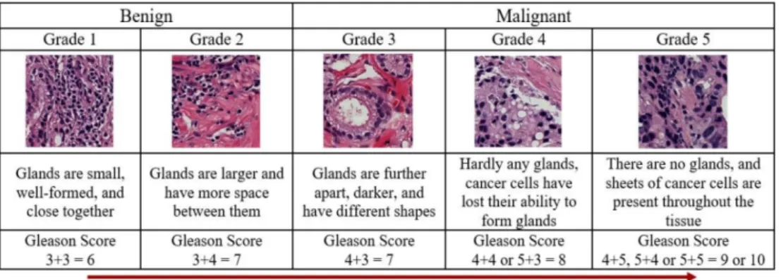
Feature extraction is very important when performing cancer grading using biopsy images. Generally, the classification of PCa grading is carried out based on morphological, texture, nuclei cluster, architectural, and colour moment features. However, the current study focuses on wavelet transformation and colour histogram analysis for stained biopsy tissue image processing. At present, automated computerised techniques are in high demand for medical image analysis and processing, and the multilayer perceptron (MLP) is a commonly used technique for feature classification. Texture and colour features are highly significant in tissue image analysis and provide information about the intensity and distribution of colour in an image. The arrangement of the glands and cell nuclei in tissue images and their shape and size differ among Gleason grade groups, shown in Figure1. The research is presented in five sections. First, a discrete wavelet transform (DWT) was performed on each pathology image using the Haar wavelet function. Second, the grey level co-occurrence matrix (GLCM) was calculated to extract texture features from the wavelet-transformed images. Third, RGB (red/green/blue) colour images were converted and separated into three channels of 8 bits/pixel
Cancers2019,11, 1937 3 of 21
each. Fourth, the colour distribution of each channel was analysed, and colour moment features were extracted. Fifth, the significant features were selected and classified for predicting cancer grading in histological sections of prostate carcinomas.
Cancers 2019, 11, x 3 of 22
extracted. Fifth, the significant features were selected and classified for predicting cancer grading in histological sections of prostate carcinomas.
Figure 1. Gleason scores and prostate cancer grading system. The Gleason score for cancer grading is computed by adding the primary and secondary scores from a whole slide H&E-stained microscopic biopsy image. The cancer detection process in histopathology consists of categorising stained microscopic biopsy images into benign and malignant. The Gleason score predicts the aggressiveness of prostate cancer. The images used for Grade 1-5 were scanned at 40× optical magnification, respectively. 2. Materials and Methods
Ethical Approval:All subjects’ written informed consent waived for their participation in the study, which was approved by the Institutional Ethics Committee at College of Medicine, Yonsei University, Korea (IRB no. 1-2018-0044).
2.1. Dataset Preparation
Prostate tissue images were obtained from the Severance Hospital of Yonsei University in Seoul, Korea. The size of the whole slide image was 33,584 × 70,352 pixels. These slides were scanned into a computer workstation at 40× optical magnification with a 0.3 NA objective using a digital camera (Olympus C-3000) attached to a microscope (Olympus BX-51), and images were cropped to a size of 512 × 512 pixels and 256 × 256 pixels. We used a total of 400 samples with an image size of 256 × 256 pixels, and each image slice had a resolution of 24 bits/pixel. The collected samples were divided into four groups: benign, grade 3, grade 4, and grade 5. The biopsy tissue was sectioned in 4 μm and the sections were deparaffinized, rehydrated, and stained with hematoxylin and eosin (H&E) using an automated stainer (Leica Autostainer XL). The colour dyes are typically used by pathologists to visualise and analyse tissue components, such as stroma, cytoplasm, nucleus, and lumen.
The H&E stain has been used for over a century and remains essential for identifying different tissue types. This stain reveals a broad range of nuclear, cytoplasmic, and extracellular-matrix features. Briefly, haematoxylin is used in combination with a “mordant”, which is a compound that helps it associate with the tissue. This compound is also called “hematin”, which is positively charged and can react with negatively charged, basophilic cell components, such as nucleic acids in the nucleus. The stain colour for this compound is blue, and the chemical formula is C16H24O6. Eosin is negatively charged and can react with positively charged, acidophilic components, such as amino groups in proteins in the cytoplasm. The stain colour for this compound is pink, and the chemical formula is C20H6Br4Na2O5. The detail explanation of cell block preparation, tissue processing, and immunocytochemical analysis is in Appendix A. Figures A1 and A2 shows H&E straining slide images and the cropped images extracted from whole slides tissue images, recpectively.
2.2. Proposed Pipeline for Analysis and Classification
MLP classification was performed using a combination of features extracted from microscopic biopsy images of tissue samples. We used a DWT algorithm for wavelet decomposition and computed the GLCM to extract texture features. Colour-feature extraction was also carried out for
Figure 1.Gleason scores and prostate cancer grading system. The Gleason score for cancer grading is computed by adding the primary and secondary scores from a whole slide H&E-stained microscopic biopsy image. The cancer detection process in histopathology consists of categorising stained microscopic biopsy images into benign and malignant. The Gleason score predicts the aggressiveness of prostate cancer. The images used for Grade 1–5 were scanned at 40×optical magnification, respectively. 2. Materials and Methods
Ethical Approval: All subjects’ written informed consent waived for their participation in the study, which was approved by the Institutional Ethics Committee at College of Medicine, Yonsei University, Korea (IRB no. 1-2018-0044).
2.1. Dataset Preparation
Prostate tissue images were obtained from the Severance Hospital of Yonsei University in Seoul, Korea. The size of the whole slide image was 33,584×70,352 pixels. These slides were scanned into a computer workstation at 40×optical magnification with a 0.3 NA objective using a digital camera (Olympus C-3000) attached to a microscope (Olympus BX-51), and images were cropped to a size of 512×512 pixels and 256×256 pixels. We used a total of 400 samples with an image size of 256×256 pixels, and each image slice had a resolution of 24 bits/pixel. The collected samples were divided into four groups: benign, grade 3, grade 4, and grade 5. The biopsy tissue was sectioned in 4µm and the sections were deparaffinized, rehydrated, and stained with hematoxylin and eosin (H&E) using an automated stainer (Leica Autostainer XL). The colour dyes are typically used by pathologists to visualise and analyse tissue components, such as stroma, cytoplasm, nucleus, and lumen.
The H&E stain has been used for over a century and remains essential for identifying different tissue types. This stain reveals a broad range of nuclear, cytoplasmic, and extracellular-matrix features. Briefly, haematoxylin is used in combination with a “mordant”, which is a compound that helps it associate with the tissue. This compound is also called “hematin”, which is positively charged and can react with negatively charged, basophilic cell components, such as nucleic acids in the nucleus. The stain colour for this compound is blue, and the chemical formula is C16H24O6. Eosin is negatively charged and can react with positively charged, acidophilic components, such as amino groups in proteins in the cytoplasm. The stain colour for this compound is pink, and the chemical formula is C20H6Br4Na2O5. The detail explanation of cell block preparation, tissue processing, and immunocytochemical analysis is in AppendixA. FiguresA1andA2shows H&E straining slide images and the cropped images extracted from whole slides tissue images, recpectively.
Cancers2019,11, 1937 4 of 21
2.2. Proposed Pipeline for Analysis and Classification
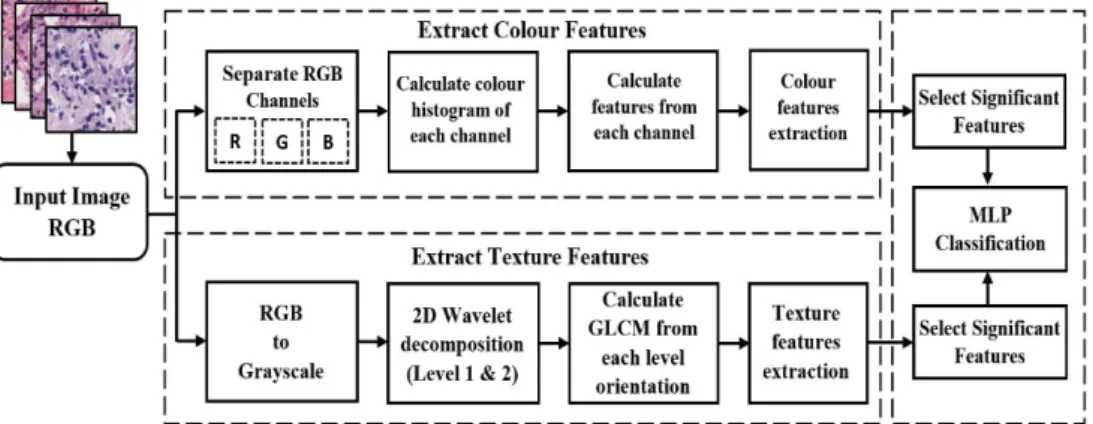
MLP classification was performed using a combination of features extracted from microscopic biopsy images of tissue samples. We used a DWT algorithm for wavelet decomposition and computed the GLCM to extract texture features. Colour-feature extraction was also carried out for PCa grading. These features are suitable for the different pathology categories for image analysis chosen for the study. After Haar wavelet transformation, we generated the first and second levels of images and extracted features from each level depth. Artificial neural network (ANN) classification methods were used to classify prostate carcinomas. The proposed methodology in Figure2shows the process for extracting colour and texture features from an input image and performing MLP classification using the significant features. MANOVA statistical test was carried out in RStudio development environment, to select the most significant features for classification. This proposed method is expected to improve the classification accuracy rate compared with the method described in our previously published paper.
Cancers 2019, 11, x 4 of 22
PCa grading. These features are suitable for the different pathology categories for image analysis chosen for the study. After Haar wavelet transformation, we generated the first and second levels of images and extracted features from each level depth. Artificial neural network (ANN) classification methods were used to classify prostate carcinomas. The proposed methodology in Figure 2 shows the process for extracting colour and texture features from an input image and performing MLP classification using the significant features. MANOVA statistical test was carried out in RStudio development environment, to select the most significant features for classification. This proposed method is expected to improve the classification accuracy rate compared with the method described in our previously published paper.
Figure 2. Proposed method for PCa grading in histological sections based on wavelet texture and colour features. Each section is analysed individually and separately for better understanding. Both colour and texture features extraction methods are analysed and performed using grayscale images, which are converted from RGB color images. In the final step, the significant features are selected and classified using an MLP neural network classification algorithm.
2.3. Discrete Wavelet Transform
Wavelet functions are concentrated in time as well as in frequency around a certain point. The wavelet transform is most appropriate for non-stationary signals and basic functions, which vary both in frequency and spatial range. The wavelet transform is designed to provide good frequency resolution for low-frequency components, which are essentially the average intensity values of the image, and high temporal resolution for high-frequency components, which are basically the edges of the image. In the present study, a DWT was performed to divide the information of an image into approximation and detailed sub-signals and extract the most discriminative multi-scale features [6]. In Figure 3, the approximation sub-signal shows the general trend of pixel values, and the detailed sub-signal shows the horizontal, vertical, and diagonal details. Figure 3 shows the two-dimensional first- and second-level wavelet decomposition, in which the original image is the input image for first-level transformation (LL1, LH1, HL1, HH1), and the approximation image (LL1) was used as the input image for second-level transformation (LL2, LH2, HL2, HH2). Figure 4 shows the structure of the first- and second-level wavelet transformation presented in Figure 3, respectively. The input image for the first- and second-level transformations was downsampled by 2, which changed the resolution of the sub-images. The sub-signals of the two-dimensional wavelet decomposition in Figure 4 were computed using the following Equations (1)–(4), respectively [7].
Figure 2.Proposed method for PCa grading in histological sections based on wavelet texture and colour features. Each section is analysed individually and separately for better understanding. Both colour and texture features extraction methods are analysed and performed using grayscale images, which are converted from RGB color images. In the final step, the significant features are selected and classified using an MLP neural network classification algorithm.
2.3. Discrete Wavelet Transform
Wavelet functions are concentrated in time as well as in frequency around a certain point. The wavelet transform is most appropriate for non-stationary signals and basic functions, which vary both in frequency and spatial range. The wavelet transform is designed to provide good frequency resolution for low-frequency components, which are essentially the average intensity values of the image, and high temporal resolution for high-frequency components, which are basically the edges of the image. In the present study, a DWT was performed to divide the information of an image into approximation and detailed sub-signals and extract the most discriminative multi-scale features [6]. In Figure3, the approximation sub-signal shows the general trend of pixel values, and the detailed sub-signal shows the horizontal, vertical, and diagonal details. Figure3shows the two-dimensional first- and second-level wavelet decomposition, in which the original image is the input image for first-level transformation (LL1, LH1, HL1, HH1), and the approximation image (LL1) was used as the input image for second-level transformation (LL2, LH2, HL2, HH2). Figure4shows the structure of the first- and second-level wavelet transformation presented in Figure3, respectively. The input image for the first- and second-level transformations was downsampled by 2, which changed the resolution of the sub-images. The sub-signals of the two-dimensional wavelet decomposition in Figure4were computed using the following Equations (1)–(4), respectively [7].
Cancers2019,11, 1937 5 of 21 WψA(j,m,n) = √1 MN M−1 X x=0 N−1 X y=0 f(x,y)ψAj 1,m,n (1) WVφ(j,m,n) = √1 MN M−1 X x=0 N−1 X y=0 f(x,y)φVj,m,n (2) WφH(j,m,n) = √1 MN M−1 X x=0 N−1 X y=0 f(x,y)φHj,m,n (3) WDφ(j,m,n) = √1 MN M−1 X x=0 N−1 X y=0 f(x,y)φDj,m,n (4) whereψAj 1,m,n(x,y)andφ i
j,m,n(x,y)describe the two-dimensional wavelet functions of leveljat pixel in
rowmand columnnof an input image with rowsMand columnsNnumber of pixels,Arepresent an approximation orientation andirepresents the other orientation of wavelet details coefficients, namely vertical, horizontal, and diagonal.Cancers 2019, 11, x 5 of 22
Figure 3. The process of constructing from level-1 to level-2 wavelet transformation. A sequence of two low-pass and high-pass filters, 2Lo_D (row, column) and 2Hi_D (row, column) followed by downsampling provides the approximation and diagonal sub-images, respectively. A combination of low- and high-pass filters and downsamplings provides the vertical and horizontal sub-images.
Figure 3. The process of constructing from level-1 to level-2 wavelet transformation. A sequence of two low-pass and high-pass filters, 2Lo_D (row, column) and 2Hi_D (row, column) followed by downsampling provides the approximation and diagonal sub-images, respectively. A combination of low- and high-pass filters and downsamplings provides the vertical and horizontal sub-images.
Cancers 2019, 11, x 6 of 22
Figure 4. Two-dimensional first- and second-level wavelet decomposition of an input image. (a) Input image of size 256 × 256 pixels. (b) Structure of level-1 wavelet transform, each sub-image (LL1, LH1, HL1, HH1) has 128 × 128 pixels in size. (c) Structure of level-2 wavelet transform, each sub-image (LL2, LH2, HL2, HH2) has 64 × 64 pixels in size.
𝑊 (𝑗, 𝑚, 𝑛) = 1 √𝑀𝑁 𝑓(𝑥, 𝑦)𝜓 , , (1) 𝑊 (𝑗, 𝑚, 𝑛) = 1 √𝑀𝑁 𝑓(𝑥, 𝑦)𝜙, , (2) 𝑊 (𝑗, 𝑚, 𝑛) = 1 √𝑀𝑁 𝑓(𝑥, 𝑦)𝜙, , (3) 𝑊 (𝑗, 𝑚, 𝑛) = 1 √𝑀𝑁 𝑓(𝑥, 𝑦)𝜙, , (4)
where 𝜓 , , (𝑥, 𝑦) and 𝜙, , (𝑥, 𝑦) describe the two-dimensional wavelet functions of level 𝑗 at
pixel in row 𝑚 and column 𝑛 of an input image with rows 𝑀 and columns 𝑁 number of pixels,
𝐴 represent an approximation orientation and 𝑖 represents the other orientation of wavelet details coefficients, namely vertical, horizontal, and diagonal.
2.3.1. Haar Wavelet Transform
The simplest type of wavelet transform is called a Haar wavelet. It is related to a mathematical operation called the Haar transform. It is performed in several stages, or levels. Haar transform decomposes a discrete signal into two sub-signals of half its length [8,9]. One sub-signal is a running average, and the other sub-signal is a running difference, storing details coefficients, eliminating data, and reconstructing the matrix such that the resulting matrix is similar to the initial matrix. The low-pass (Lo_D) and high-pass (Hi_D) filters are given by Lo_D = √ ,√ and Hi_D = √ , −√ which are basically used for Haar wavelet transformation [10,11]. Figure 5 shows the multilevel wavelet transformed images of prostate carcinomas, and this implementation was carried out in MATLAB R2018a, where a 24-bit RGB color image was converted into 8-bit for processing the image.
There are two functions that play a primary role in wavelet analysis, the scaling function 𝜙 (father wavelet) and the wavelet function 𝜓 (mother wavelet), shown in Figure 6. In the Haar wavelet transform, the scaling and wavelet functions can be treated as extractors of particular image features. The scaling and wavelet functions in Figure 6 were constructed based on the unit interval (0 to 1) and (−1 to 1), respectively. Haar scaling and wavelet function can be described as
Father Wavelet 𝜙(𝑥) = 1 𝑓𝑜𝑟 0 ≤ 𝑥 < 1 0 𝑜𝑡ℎ𝑒𝑟𝑤𝑖𝑠𝑒 (5) Mother Wavelet 𝜓(𝑥) = 1 𝑓𝑜𝑟 0 ≤ 𝑥 < 1/2 −1 𝑓𝑜𝑟 1/2 ≤ 𝑥 < 1 0 𝑜𝑡ℎ𝑒𝑟𝑤𝑖𝑠𝑒 (6)
Figure 4.Two-dimensional first- and second-level wavelet decomposition of an input image. (a) Input image of size 256×256 pixels. (b) Structure of level-1 wavelet transform, each sub-image (LL1, LH1, HL1, HH1) has 128×128 pixels in size. (c) Structure of level-2 wavelet transform, each sub-image (LL2, LH2, HL2, HH2) has 64×64 pixels in size.
Haar Wavelet Transform
The simplest type of wavelet transform is called a Haar wavelet. It is related to a mathematical operation called the Haar transform. It is performed in several stages, or levels. Haar transform decomposes a discrete signal into two sub-signals of half its length [8,9]. One sub-signal is a running
Cancers2019,11, 1937 6 of 21
average, and the other sub-signal is a running difference, storing details coefficients, eliminating data, and reconstructing the matrix such that the resulting matrix is similar to the initial matrix. The low-pass (Lo_D) and high-pass (Hi_D) filters are given by Lo_D =
1 √ 2, 1 √ 2 and Hi_D= 1 √ 2, − 1 √ 2 which are basically used for Haar wavelet transformation [10,11]. Figure5shows the multilevel wavelet transformed images of prostate carcinomas, and this implementation was carried out in MATLAB R2018a, where a 24-bit RGB color image was converted into 8-bit for processing the image.Cancers 2019, 11, x 7 of 22
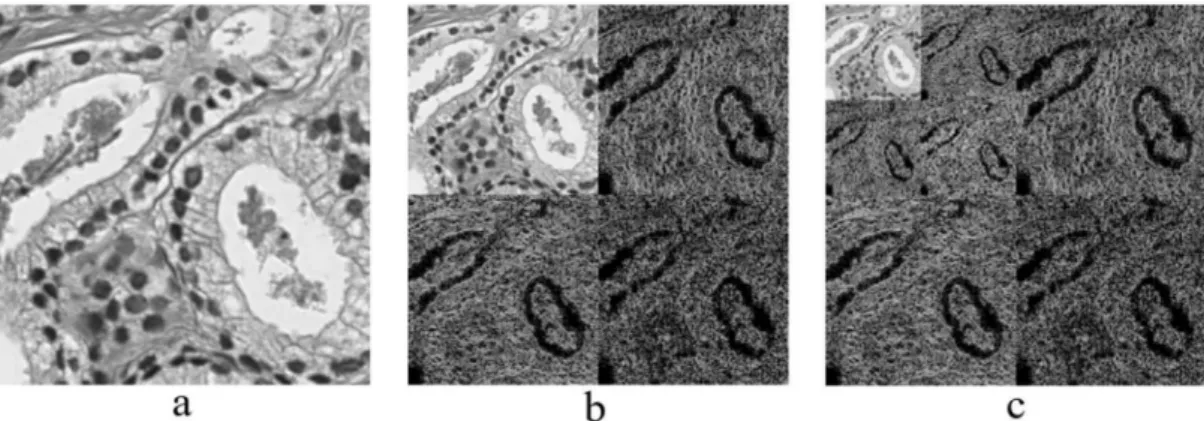
Figure 5. Haar wavelet transformation.(a) Original image converted from RGB to grayscale, which was cropped from a whole slide tissue image and scanned at 40× optical magnification. (b) Level-1 wavelet decomposition. (c) Level-2 wavelet decomposition.
Figure 5.Haar wavelet transformation. (a) Original image converted from RGB to grayscale, which was cropped from a whole slide tissue image and scanned at 40×optical magnification. (b) Level-1 wavelet decomposition. (c) Level-2 wavelet decomposition.
There are two functions that play a primary role in wavelet analysis, the scaling functionφ (father wavelet) and the wavelet functionψ(mother wavelet), shown in Figure6. In the Haar wavelet transform, the scaling and wavelet functions can be treated as extractors of particular image features. The scaling and wavelet functions in Figure6were constructed based on the unit interval (0 to 1) and (−1 to 1), respectively. Haar scaling and wavelet function can be described as
Father Waveletφ(x) = ( 1 f or0≤x<1 0 otherwise (5) Mother Waveletψ(x) = 1 f or0≤x<1/2 −1 f or1/2≤x<1 0 otherwise (6) Cancers 2019, 11, x 8 of 22
Figure 6. (a) Haar scaling function (Father Wavelet). (b) Haar wavelet function (Mother Wavelet). 2.4. Color Moment Analysis
In colour moment analysis, a colour histogram is used to represent the colour distribution in microscopic biopsy tissue images. Colour information is a very important factor for tissue image analysis, and each peak of the histogram represents a different colour, as shown in Figure 7. In Figure 7e–h, the x-axis and y-axis of the colour histogram show the number of bins and colour pixels present in an image, respectively. Colour moment analysis was carried out to extract colour-based features from prostate tissue images [12].
Figure 7. Sample microscopic biopsy images of prostate tissue. (a–d) Prostate tissue images of benign, grade 3, grade 4, and grade 5 based on the Gleason grading system, respectively. These images were scanned at 40× optical magnification. (e–h) Colour histograms in RGB colour space are generated from the tissue images in (a–d), respectively.
Colour moment analysis is essential in digital medical image processing to carry out colour image enhancement or information retrieval. Figure 7e–h shows the colour information of each individual channel present in the prostate tissue images of Figure 7a–d, respectively. We computed the percentage of each individual colour in the RGB channel using the following formula:
Colour Percentage % =𝑇𝑜𝑡𝑎𝑙 𝑛𝑢𝑚𝑏𝑒𝑟 𝑐𝑜𝑙𝑜𝑢𝑟 𝑐ℎ𝑎𝑛𝑛𝑛𝑒𝑙 𝑝𝑖𝑥𝑒𝑙𝑠
𝑇𝑜𝑡𝑎𝑙 𝑛𝑢𝑚𝑏𝑒𝑟 𝑜𝑓 𝑖𝑚𝑎𝑔𝑒 𝑝𝑖𝑥𝑒𝑙𝑠 × 100 (7)
2.5. Feature Extraction
Two-dimensional (2D) grey-level co-occurrence matrix (GLCM) and colour moment techniques were used to extract texture and pixel-based colour moment features, respectively. Texture features were extracted from Haar wavelet-transformed images, and colour features were extracted from 8-bit grayscale images that were separated into three channels from an original colour image. We extracted
Figure 6.(a) Haar scaling function (Father Wavelet). (b) Haar wavelet function (Mother Wavelet). 2.4. Color Moment Analysis
In colour moment analysis, a colour histogram is used to represent the colour distribution in microscopic biopsy tissue images. Colour information is a very important factor for tissue image analysis, and each peak of the histogram represents a different colour, as shown in Figure7.
Cancers2019,11, 1937 7 of 21
In Figure7e–h, the x-axis and y-axis of the colour histogram show the number of bins and colour pixels present in an image, respectively. Colour moment analysis was carried out to extract colour-based features from prostate tissue images [12].
Cancers 2019, 11, x 8 of 22
Figure 6. (a) Haar scaling function (Father Wavelet). (b) Haar wavelet function (Mother Wavelet). 2.4. Color Moment Analysis
In colour moment analysis, a colour histogram is used to represent the colour distribution in microscopic biopsy tissue images. Colour information is a very important factor for tissue image analysis, and each peak of the histogram represents a different colour, as shown in Figure 7. In Figure 7e–h, the x-axis and y-axis of the colour histogram show the number of bins and colour pixels present in an image, respectively. Colour moment analysis was carried out to extract colour-based features from prostate tissue images [12].
Figure 7. Sample microscopic biopsy images of prostate tissue. (a–d) Prostate tissue images of benign, grade 3, grade 4, and grade 5 based on the Gleason grading system, respectively. These images were scanned at 40× optical magnification. (e–h) Colour histograms in RGB colour space are generated from the tissue images in (a–d), respectively.
Colour moment analysis is essential in digital medical image processing to carry out colour image enhancement or information retrieval. Figure 7e–h shows the colour information of each individual channel present in the prostate tissue images of Figure 7a–d, respectively. We computed the percentage of each individual colour in the RGB channel using the following formula:
Colour Percentage % =𝑇𝑜𝑡𝑎𝑙 𝑛𝑢𝑚𝑏𝑒𝑟 𝑐𝑜𝑙𝑜𝑢𝑟 𝑐ℎ𝑎𝑛𝑛𝑛𝑒𝑙 𝑝𝑖𝑥𝑒𝑙𝑠𝑇𝑜𝑡𝑎𝑙 𝑛𝑢𝑚𝑏𝑒𝑟 𝑜𝑓 𝑖𝑚𝑎𝑔𝑒 𝑝𝑖𝑥𝑒𝑙𝑠 × 100 (7)
2.5. Feature Extraction
Two-dimensional (2D) grey-level co-occurrence matrix (GLCM) and colour moment techniques were used to extract texture and pixel-based colour moment features, respectively. Texture features were extracted from Haar wavelet-transformed images, and colour features were extracted from 8-bit grayscale images that were separated into three channels from an original colour image. We extracted
Figure 7.Sample microscopic biopsy images of prostate tissue. (a–d) Prostate tissue images of benign, grade 3, grade 4, and grade 5 based on the Gleason grading system, respectively. These images were scanned at 40×optical magnification. (e–h) Colour histograms in RGB colour space are generated from the tissue images in (a–d), respectively.
Colour moment analysis is essential in digital medical image processing to carry out colour image enhancement or information retrieval. Figure7e–h shows the colour information of each individual channel present in the prostate tissue images of Figure7a–d, respectively. We computed the percentage of each individual colour in the RGB channel using the following formula:
Colour Percentage[%] = Total number colour channnel pixels
Total number o f image pixels ×100 (7) 2.5. Feature Extraction
Two-dimensional (2D) grey-level co-occurrence matrix (GLCM) and colour moment techniques were used to extract texture and pixel-based colour moment features, respectively. Texture features were extracted from Haar wavelet-transformed images, and colour features were extracted from 8-bit grayscale images that were separated into three channels from an original colour image. We extracted a total of 11 features and carried out a multivariate analysis of variance (MANOVA) statistical test to identify the significant features [13–16].
2.5.1. Texture Features
GLCM is a statistical method that examines texture based on the spatial relationship of pixels. To analyse image texture, we first created a GLCM to calculate how often pairs of pixels with specific values and in a specified spatial relationship occurred in an image, and then extracted statistical measures from the matrix. The directions of the co-occurrence matrix for feature extraction were as follows: 0◦[0, 1], 45◦[−1, 1], 90◦[−1, 0], and 135◦[−1,−1]. So, the values of GLCM matrix are always within the range [0, 1]. The size of the GLCM matrix used for texture analysis was 128×128 and 64×64, for first- and second-level sub-images, respectively. GLCM texture features were separately extracted after wavelet transformation at level-1 and level-2 from each orientation, shown in Figure8. Based on the GLCM, we computed six different types of wavelet texture features: contrast, homogeneity,
Cancers2019,11, 1937 8 of 21
correlation, energy, entropy, and dissimilarity [17–20]. These features were calculated using the following equations: Contrast= N−1 X i=0 N−1 X j=0 i−j 2 p(i−j) (8) Homogeneity= N−1 X i=0 N−1 X j=0 p(i,j) 1+ (i+j)2 (9) Correlation= N−1 X i=0 N−1 X j=0 p(i,j)(i −µx)i−µy σxσy (10) Energy= N−1 X i=0 N−1 X j=0 p(i,j)2 (11) Entropy=− N−1 X i=0 N−1 X j=0 p(i,j) log(p(i,j)) (12) Dissimilarity= N−1 X i=0 N−1 X j=0 i−j p(i−j) (13)
wherep(i–j) signifies the co-occurrence probability matrix for a combination of two pixels with intensity (i,j) that occur in an image, separated by a given distance. Nsignifies the quantized grey level, andµxandµyare the means, andσxandσythe standard deviations, for rowiand columnj, respectively, within the GLCM.
Cancers 2019, 11, x 9 of 22
a total of 11 features and carried out a multivariate analysis of variance (MANOVA) statistical test to identify the significant features [13–16].
2.5.1. Texture Features
GLCM is a statistical method that examines texture based on the spatial relationship of pixels. To analyse image texture, we first created a GLCM to calculate how often pairs of pixels with specific values and in a specified spatial relationship occurred in an image, and then extracted statistical measures from the matrix. The directions of the co-occurrence matrix for feature extraction were as follows: 0° [0, 1], 45° [−1, 1], 90° [−1, 0], and 135° [−1, −1]. So, the values of GLCM matrix are always within the range [0, 1]. The size of the GLCM matrix used for texture analysis was 128 × 128 and 64 × 64, for first- and second-level sub-images, respectively. GLCM texture features were separately extracted after wavelet transformation at level-1 and level-2 from each orientation, shown in Figure 8. Based on the GLCM, we computed six different types of wavelet texture features: contrast, homogeneity, correlation, energy, entropy, and dissimilarity [17–20]. These features were calculated using the following equations:
𝐶𝑜𝑛𝑡𝑟𝑎𝑠𝑡 = |𝑖 − 𝑗| 𝑝(𝑖 − 𝑗) (8) 𝐻𝑜𝑚𝑜𝑔𝑒𝑛𝑒𝑖𝑡𝑦 = 𝑝(𝑖, 𝑗) 1 + (𝑖 + 𝑗) (9) 𝐶𝑜𝑟𝑟𝑒𝑙𝑎𝑡𝑖𝑜𝑛 = 𝑝(𝑖, 𝑗)(𝑖 − 𝜇 )(𝑖 − 𝜇 )𝜎 𝜎 (10) 𝐸𝑛𝑒𝑟𝑔𝑦 = 𝑝(𝑖, 𝑗) (11) 𝐸𝑛𝑡𝑟𝑜𝑝𝑦 = − 𝑝(𝑖, 𝑗) log (𝑝(𝑖, 𝑗)) (12) 𝐷𝑖𝑠𝑠𝑖𝑚𝑖𝑙𝑎𝑟𝑖𝑡𝑦 = |𝑖 − 𝑗|𝑝(𝑖 − 𝑗) (13)
where p(i – j) signifies the co-occurrence probability matrix for a combination of two pixels with intensity (i, j) that occur in an image, separated by a given distance. N signifies the quantized grey level, and µx and µy are the means, and 𝜎 and 𝜎 the standard deviations, for row i and column j, respectively, within the GLCM.
Figure 8.Level-1 and level-2 Haar wavelet texture images. (a–d) First-level orientation sub-images, each 128×128 pixels in size. (e–h) Second-level orientation sub-images, each 64×64 pixels in size. From level-1 and level-2, (a,e), (b,f), (c,g) and (d,h) represents the wavelet coefficients, which includes approximation, vertical, horizontal, and diagonal, respectively.
2.5.2. Colour Moment Features
The pixel-based colour moment descriptor (PCMD) technique was used to extract colour-based features from prostate tissue images. This technique is useful for analysing the colour distribution among the three different channels of RGB colour images. To extract useful colour moment features from tissue images, the three colour channels were separated from RGB colour images, as shown in
Cancers2019,11, 1937 9 of 21
Figure9. We then computed the mean, standard deviation, skewness, variance, and kurtosis from each individual channel separately [21,22]. These features were calculated using the following equations:
Mean(µi) = N X j=1 1 Npi j (14)
Standard deviation(σi) = v u t (1 N 1 X N pi j−µi 2 ) (15) Skewness(si) = 3 v u t (1 N 1 X N pi j−µi 3 ) (16) Kurtosis(ki) = 4 v u t (1 N 1 X N pi j−µi 4 ) (17)
where,pi jis the value ofjthpixel of the image at theithcolor channel. Nis the number of pixels in the
image.µiis the mean value,σi. is the standard deviation and it is obtained by taking the square root of the variance of the color distribution,siis the skewness, andkiis the kurtosis.
Cancers 2019, 11, x 10 of 22
Figure 8. Level-1 and level-2 Haar wavelet texture images. (a–d) First-level orientation sub-images, each 128 × 128 pixels in size. (e–h) Second-level orientation sub-images, each 64 × 64 pixels in size. From level-1 and level-2, (a,e), (b,f), (c,g) and (d,h) represents the wavelet coefficients, which includes approximation, vertical, horizontal, and diagonal, respectively.
2.5.2. Colour Moment Features
The pixel-based colour moment descriptor (PCMD) technique was used to extract colour-based features from prostate tissue images. This technique is useful for analysing the colour distribution among the three different channels of RGB colour images. To extract useful colour moment features from tissue images, the three colour channels were separated from RGB colour images, as shown in Figure 9. We then computed the mean, standard deviation, skewness, variance, and kurtosis from each individual channel separately [21,22]. These features were calculated using the following equations: 𝑀𝑒𝑎𝑛 (𝜇 ) = 1 𝑁𝑝 (14) 𝑆𝑡𝑎𝑛𝑑𝑎𝑟𝑑 𝑑𝑒𝑣𝑖𝑎𝑡𝑖𝑜𝑛 (𝜎 ) = (1 𝑁 (𝑝 − 𝜇 ) ) (15) 𝑆𝑘𝑒𝑤𝑛𝑒𝑠𝑠 (𝑠 ) = (𝑁1 (𝑝 − 𝜇 ) ) (16) 𝐾𝑢𝑟𝑡𝑜𝑠𝑖𝑠 (𝑘 ) = (1 𝑁 (𝑝 − 𝜇 ) ) (17)
where, 𝑝 is the value of 𝑗 pixel of the image at the 𝑖 color channel. 𝑁 is the number of pixels in the image. 𝜇 is the mean value, 𝜎 is the standard deviation and it is obtained by taking the square root of the variance of the color distribution, 𝑠 is the skewness, and 𝑘 is the kurtosis.
Figure 9. Tissue image processing and colour moment analysis by splitting RGB colour channels. (a) Original RGB tissue image stained with H&E compunds. (b) The red, green and blue component converted from an original image (a) with the resolution of 24-bits/pixel. (c) The respective split channels of R, G and B images present in (b). Specifically, these images are formed by converting each 24-bit R, G and B images into 8-bit grayscale images, respectively. (d) The extracted features from each color channel present in (c), respectively.
2.6. MLP Classification
MLP is a supervised classification system that consists of at least three layers of nodes: the first layer is the input layer, the middle layer is the hidden layer, and the last layer is the output layer. Input and output layers are used to feed in data and obtain the output results, respectively [23–26]. However, the hidden layer can be modified to increase the complexity of the model. It is a feed-forward ANN, in which each node is a neuron of hidden and output layers and uses a nonlinear activation function. To carry out PCa grading, binary classification was performed using the MLP neural network classifier in Waikato Environment (WEKA), which classified the samples as benign vs. malignant, benign vs. grade 3, benign vs. grade 4, benign vs. grade 5, and grade 3 vs. grade 4,5. WEKA was developed at the University of Waikato, New Zealand. It supports many data mining tasks, such as classification, clustering, regression, and feature selection [27].
Cancers2019,11, 1937 10 of 21
To train the model, we input data into the model, multiplied the data with the weights, and obtained the computed output of the model, which is called a forward pass. We also carried out backward passes, in which model weight was updated based on the calculated loss from the expected and predicted outputs. The learning rate is a hyperparameter in the neural network that controls how the model is changed in response to the estimated error each time the model weight is updated based on the learning rate and momentum. Momentum is a technique that frequently improves both training speed and accuracy [28,29]. The activation function used for the training process was the sigmoid function, which takes an input value and squashes it to within the range of 0 and 1, to perform binary classification. We designed the network with one input layer, two hidden layers, and one output layer, shown in Figure10. The weight was updated automatically while training the model based on the following equations:
w=w+learning rate∗(expected−predicted)∗n (18) z=
n
X
i=1
wixi+biasSigmoid Function : f(z) = 1
1+exp−z (19)
wherewis the weight,nis the number of features in x, and z is the linear form of equation used in the sigmoid function, to generate non-linear activation function.
Cancers 2019, 11, x 11 of 22
MLP is a supervised classification system that consists of at least three layers of nodes: the first layer is the input layer, the middle layer is the hidden layer, and the last layer is the output layer. Input and output layers are used to feed in data and obtain the output results, respectively [23–26]. However, the hidden layer can be modified to increase the complexity of the model. It is a feed-forward ANN, in which each node is a neuron of hidden and output layers and uses a nonlinear activation function. To carry out PCa grading, binary classification was performed using the MLP neural network classifier in Waikato Environment (WEKA), which classified the samples as benign vs. malignant, benign vs. grade 3, benign vs. grade 4, benign vs. grade 5, and grade 3 vs. grade 4,5. WEKA was developed at the University of Waikato, New Zealand. It supports many data mining tasks, such as classification, clustering, regression, and feature selection [27].
To train the model, we input data into the model, multiplied the data with the weights, and obtained the computed output of the model, which is called a forward pass. We also carried out backward passes, in which model weight was updated based on the calculated loss from the expected and predicted outputs. The learning rate is a hyperparameter in the neural network that controls how the model is changed in response to the estimated error each time the model weight is updated based on the learning rate and momentum. Momentum is a technique that frequently improves both training speed and accuracy [28,29]. The activation function used for the training process was the sigmoid function, which takes an input value and squashes it to within the range of 0 and 1, to perform binary classification. We designed the network with one input layer, two hidden layers, and one output layer, shown in Figure 10. The weight was updated automatically while training the model based on the following equations:
𝑤 = 𝑤 + 𝑙𝑒𝑎𝑟𝑛𝑖𝑛𝑔 𝑟𝑎𝑡𝑒 ∗ (𝑒𝑥𝑝𝑒𝑐𝑡𝑒𝑑 − 𝑝𝑟𝑒𝑑𝑖𝑐𝑡𝑒𝑑) ∗ 𝑛 (18)
z = 𝑤𝑖𝑥𝑖 + 𝑏𝑖𝑎𝑠 Sigmoid Function: f(z) = 1
1 + 𝑒𝑥𝑝
(19)
where 𝑤 is the weight, 𝑛 is the number of features in x, and z is the linear form of equation used in the sigmoid function, to generate non-linear activation function.
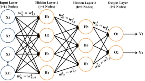
Figure 10. MLP classifier model with input, hidden, and output layers. The input layer contains 11 nodes, the output layer contains 2 nodes, and hidden layers 1 and 2 contain 4 and 3 nodes, respectively. The perceptron takes 11 input features (X1–X11) extracted from prostate tissue images, and weights (W1–W3) are associated with those inputs. The network performs a weighted summation to produce an output Y, and perceptron weight is determined during the training process based on training data.
3. Results and Discussion
In the present study, we extracted wavelet-based texture and colour moment features for MLP neural network classification. Images were 256 × 256 pixels (24 bits/pixel) in size and were converted
Figure 10. MLP classifier model with input, hidden, and output layers. The input layer contains 11 nodes, the output layer contains 2 nodes, and hidden layers 1 and 2 contain 4 and 3 nodes, respectively. The perceptron takes 11 input features (X1–X11) extracted from prostate tissue images, and weights (W1–W3) are associated with those inputs. The network performs a weighted summation to produce an output Y, and perceptron weight is determined during the training process based on training data. 3. Results and Discussion
In the present study, we extracted wavelet-based texture and colour moment features for MLP neural network classification. Images were 256×256 pixels (24 bits/pixel) in size and were converted to 8 bits/pixel for wavelet transformation (first- and second-level), colour moment analysis, and feature extraction. A total of 400 images were used for PCa grading classification and were divided equally among four classes: benign, grade 3, grade 4, and grade 5. A ratio of 7:3 was fixed for training and test data sets, respectively. The algorithms used for image transformation, feature extraction, and classification were implemented in MATLAB R2018a and the WAIKATO environment [30,31]. We selected the most significant features based onF-values andP-values obtained from MANOVA statistical tests performed using the R programming language in RStudio. Tables1and2show the results of binary MLP classification for the five different groups of prostate carcinomas.
Cancers2019,11, 1937 11 of 21
Table 1.MLP classification performance based on level 1 wavelet texture and colour moment features.
Groups Accuracy (%) Sensitivity (%) Specificity (%) F1-Score (%) MCC (%)
Benign vs. Malignant 95.0 96.5 93.5 94.9 90.0
Benign vs. Grade 3 88.3 82.9 96.0 89.2 77.7
Benign vs. Grade 4 95.0 93.5 96.5 95.1 90.0
Benign vs. Grade 5 98.3 100.0 96.8 98.3 96.7
Grade 3 vs. Grade 4/5 85.0 95.4 76.9 80.8 69.5
Table 2.MLP classification performance based on level 2 wavelet texture and colour moment features.
Groups Accuracy (%) Sensitivity (%) Specificity (%) F1-Score (%) MCC (%)
Benign vs. Malignant 91.7 93.1 90.3 91.5 83.4 Benign vs. Grade 3 86.7 80.6 95.8 87.9 74.8 Benign vs. Grade 4 91.7 90.3 93.1 91.8 83.4 Benign vs. Grade 5 96.7 96.7 96.7 96.7 93.3 Grade 3 vs. Grade 4/5 83.3 95.4 76.3 80.8 69.2 Performance Metrics
We used a number of metrics to evaluate the performance of the classification model and deep learning algorithm, including accuracy, sensitivity, specificity, F1-score, and Matthew’s correlation coefficient (MCC). The four types of confusion matrices used for computing performance metrics were true positive (TP), true negative (TN), false positive (FP), and false negative (FN). The following metrics were used:
1. Accuracy: How many TP and TN were obtained out of all outcomes among all samples. Accuracy= TP+TN
TP+TN+FP+FN×100 (20)
2. Sensitivity:The rate of correctly classifying samples positively. Sensitivity= TP
TP+FN×100 (21)
3. Specificity: The rate of correctly classifying samples negatively. Speci f icity= TN
TN+FP×100 (22)
4. F1-score: It is calculated using a combination of the “Precision” and “Recall” metrics. The precision metric indicates how many classified samples are relevant, and the recall metric represents how many relevant samples are classified.
F1−score=2× Precision×Recall
Precision+Recall×100 (23)
5. MCC:An index of the performance binary of classification. Indicates the correlation between the observed and predicted binary classification.
MCC= p TP × TN − FP × FN
((TP + FN)(TP + FP)(TN + FN)(TN + FP))
×100 (24)
The accuracy rates listed in Tables1and2were used to construct line graphs, and the results were compared between the two classification modes, shown in Figure11. The data that can viewed in the
Cancers2019,11, 1937 12 of 21
line graph are the test accuracies of MLP neural network classification. The blue and orange graph in Figure11shows the classification performance between Tables1and2, respectively. It is clear from these results that the wavelet image features of level-1 were more reliable than those of level-2. MLP binary classification was carried out among five groups, and each group was classified independently and separately.
Cancers 2019, 11, x 13 of 22
Groups Accuracy (%) Sensitivity (%) Specificity (%) F1-Score (%) MCC (%)
Benign vs. Malignant 91.7 93.1 90.3 91.5 83.4
Benign vs. Grade 3 86.7 80.6 95.8 87.9 74.8
Benign vs. Grade 4 91.7 90.3 93.1 91.8 83.4
Benign vs. Grade 5 96.7 96.7 96.7 96.7 93.3
Grade 3 vs. Grade 4/5 83.3 95.4 76.3 80.8 69.2
Figure 11. Classification accuracy for the five binary divisions. Each group was classified separately and independently to minimise the error rate and increase the performance of the classification. MLP Classification 1 represents accuracy rates based on level-1 wavelet-based texture and colour features, and MLP Classification 2 represents accuracy rates based on level-2 wavelet-based texture and colour features.
The learning rate and momentum for each group classification changed based on the accuracy of the training and test dataset. The weighted average accuracy rates obtained from MLP Classifications 1 and 2 were 92.7% and 90.0%, respectively. The combination of texture and colour moment features in MLP Classification 1 produced the most accurate results using the neural network MLP technique. In neural network classification, the network parameters “Learning Rate” and “Momentum” were adjusted several times to accurately construct the network architecture and increase the accuracy for the test dataset. Figure 12 shows the box plots for six different classes used for MLP Classifications 1 and 2. A total of 11 features were used for histological grade classification. To construct the box plots, we used the weighted mean values for all features based on six classes: benign, grade 3, grade 4, grade 5, grades 4,5 and malignant.
Figure 11.Classification accuracy for the five binary divisions. Each group was classified separately and independently to minimise the error rate and increase the performance of the classification. MLP Classification 1 represents accuracy rates based on level-1 wavelet-based texture and colour features, and MLP Classification 2 represents accuracy rates based on level-2 wavelet-based texture and colour features.
The learning rate and momentum for each group classification changed based on the accuracy of the training and test dataset. The weighted average accuracy rates obtained from MLP Classifications 1 and 2 were 92.7% and 90.0%, respectively. The combination of texture and colour moment features in MLP Classification 1 produced the most accurate results using the neural network MLP technique. In neural network classification, the network parameters “Learning Rate” and “Momentum” were adjusted several times to accurately construct the network architecture and increase the accuracy for the test dataset. Figure12shows the box plots for six different classes used for MLP Classifications 1 and 2. A total of 11 features were used for histological grade classification. To construct the box plots, we used the weighted mean values for all features based on six classes: benign, grade 3, grade 4, grade 5, grades 4,5 and malignant.
Cancers 2019, 11, x 14 of 22
Figure 12. Comparison between the two levels of classification using wavelet texture and colour moment features. (a) Features used for classification 1. (b) Features used for Classification 2. Upper and lower whiskers are the maximum and minimum mean feature values, respectively, and the central line is the median value (50th percentile). Dots represent the mean values for each cancer type.
As shown in Figure 12a,b, the box plots of different grades varied in size based on the mean feature values. We used the test dataset to construct the box plots and compare the results between grades. The benign grade was more likely to have higher mean values than other grades. Thus, grade 3, grade 4, grade 5, and malignant classifications could be easily distinguished from benign tumours. Similarly, classification was performed for grade 3 vs. grades 4,5, but it was difficult to distinguish between them. It can be concluded that the wavelet texture features based on GLCM and colour moment features can accurately differentiate among six different classes in images of histological sections. The methodology proposed in this paper combines wavelet texture, colour feature extraction, and MLP classification, which produced the most accurate classification of prostate carcinomas. Classification using MLP techniques requires more time for data processing and optimization because the learning rate, momentum and number of hidden layers must be adjusted based on training and test accuracy. The use of the wavelet transform technique for analysis of microscopic biopsy images includes the following advantages:
a) It provides concurrent localisation in time and frequency domains.
b) Small wavelets can be used to separate fine details in an image, and large wavelets can identify coarse details.
c) An image can be de-noised without appreciable degradation.
Haar and Daubechies wavelets are usually used to extract texture features, detect multi-resolution characteristics, and for texture discrimination and pattern recognition. However, in the current study, we used Haar wavelet features extracted from the detailed coefficients of the transformed image at levels 1 and 2. These features revealed the characteristics of the image and were used for classifying grades of cancer observed in histological sections. Texture analysis has been an important topic in image processing and computer vision. This method is an important issue in many areas like object recognition, image retrieval study, medical imaging, robotics and remote sensing. RGB colour images were used to extract colour moment features from each channel depth. Colour texture extraction is critically important for microscopic biopsy image analysis of histological tissue sections. Texture is a connected set of pixels that occurs repeatedly in an image, and it provides information about the variation in the intensity of a surface by quantifying properties such as smoothness, coarseness, and regularity. Therefore, we performed an MLP classification using a combination of colour and wavelet texture features. The performance measures we used to evaluate the classification results included accuracy, sensitivity, specificity, F1-score, and MCC.
Our approach has been distinguishing different grade groups of prostate carcinoma: benign, grade 3, grade 4, and grade 5. In PCa grading system, grade 1 and grade 2 are classified as a
Figure 12. Comparison between the two levels of classification using wavelet texture and colour moment features. (a) Features used for classification 1. (b) Features used for Classification 2. Upper and lower whiskers are the maximum and minimum mean feature values, respectively, and the central line is the median value (50th percentile). Dots represent the mean values for each cancer type.
Cancers2019,11, 1937 13 of 21
As shown in Figure12a,b, the box plots of different grades varied in size based on the mean feature values. We used the test dataset to construct the box plots and compare the results between grades. The benign grade was more likely to have higher mean values than other grades. Thus, grade 3, grade 4, grade 5, and malignant classifications could be easily distinguished from benign tumours. Similarly, classification was performed for grade 3 vs. grades 4,5, but it was difficult to distinguish between them. It can be concluded that the wavelet texture features based on GLCM and colour moment features can accurately differentiate among six different classes in images of histological sections. The methodology proposed in this paper combines wavelet texture, colour feature extraction, and MLP classification, which produced the most accurate classification of prostate carcinomas. Classification using MLP techniques requires more time for data processing and optimization because the learning rate, momentum and number of hidden layers must be adjusted based on training and test accuracy. The use of the wavelet transform technique for analysis of microscopic biopsy images includes the following advantages:
(a) It provides concurrent localisation in time and frequency domains.
(b) Small wavelets can be used to separate fine details in an image, and large wavelets can identify coarse details.
(c) An image can be de-noised without appreciable degradation.
Haar and Daubechies wavelets are usually used to extract texture features, detect multi-resolution characteristics, and for texture discrimination and pattern recognition. However, in the current study, we used Haar wavelet features extracted from the detailed coefficients of the transformed image at levels 1 and 2. These features revealed the characteristics of the image and were used for classifying grades of cancer observed in histological sections. Texture analysis has been an important topic in image processing and computer vision. This method is an important issue in many areas like object recognition, image retrieval study, medical imaging, robotics and remote sensing. RGB colour images were used to extract colour moment features from each channel depth. Colour texture extraction is critically important for microscopic biopsy image analysis of histological tissue sections. Texture is a connected set of pixels that occurs repeatedly in an image, and it provides information about the variation in the intensity of a surface by quantifying properties such as smoothness, coarseness, and regularity. Therefore, we performed an MLP classification using a combination of colour and wavelet texture features. The performance measures we used to evaluate the classification results included accuracy, sensitivity, specificity, F1-score, and MCC.
Our approach has been distinguishing different grade groups of prostate carcinoma: benign, grade 3, grade 4, and grade 5. In PCa grading system, grade 1 and grade 2 are classified as a benign/normal tumor, whereas grades 3, 4, and 5 are classified as a malignant/abnormal tumor. The Gleason grade groups, we used for MLP neural network classification are: “Benign vs. Malignant”, “Benign vs. Grade 3”, “Benign vs. Grade 4”, “Benign vs. Grade 5”, and “Grade 3 vs. Grades 4,5”. We have extracted six texture features (contrast, homogeneity, correlation, energy, entropy, and dissimilarity) and five colour moment features (mean, standard deviation, variance, skewness, and kurtosis), from 40×optical magnification biopsy images. After going through this research, it is clear that an image texture carries useful diagnostic information, which is very essential for medical image processing and discrimination with benign and malignant tumors. However, the proposed features are not sufficient to identify and discriminate between benign and malignant; it is necessary to identify and discriminate them with more reliable features. We have compared our proposed approach with the other methods to show the performance accuracy of each method achieved by using different types of features and classification groups, shown in Table3.
Cancers2019,11, 1937 14 of 21
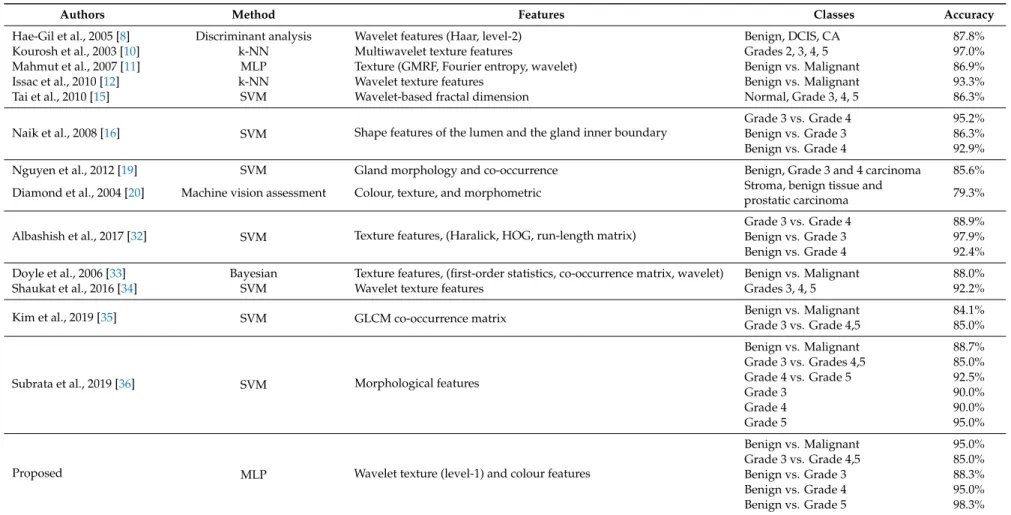
Table 3.Comparison of published methods with the proposed method for tissue characterisation. Multi-class and binary-class classifications were performed by the authors using different types of features, which were classified using machine learning techniques listed in a given table. SVM, support vector machine; k-NN, k-nearest neighbour; MLP, multilayer perceptron; GMRF, Gauss Markov random fields; HOG, histogram of oriented gradients; GLCM, gray level co-occurrence matrix; DCIS, ductal carcinoma in situ; CA, invasive ductal carcinoma.
Authors Method Features Classes Accuracy
Hae-Gil et al., 2005 [8] Discriminant analysis Wavelet features (Haar, level-2) Benign, DCIS, CA 87.8%
Kourosh et al., 2003 [10] k-NN Multiwavelet texture features Grades 2, 3, 4, 5 97.0%
Mahmut et al., 2007 [11] MLP Texture (GMRF, Fourier entropy, wavelet) Benign vs. Malignant 86.9%
Issac et al., 2010 [12] k-NN Wavelet texture features Benign vs. Malignant 93.3%
Tai et al., 2010 [15] SVM Wavelet-based fractal dimension Normal, Grade 3, 4, 5 86.3%
Naik et al., 2008 [16] SVM Shape features of the lumen and the gland inner boundary
Grade 3 vs. Grade 4 95.2%
Benign vs. Grade 3 86.3%
Benign vs. Grade 4 92.9%
Nguyen et al., 2012 [19] SVM Gland morphology and co-occurrence Benign, Grade 3 and 4 carcinoma 85.6%
Diamond et al., 2004 [20] Machine vision assessment Colour, texture, and morphometric Stroma, benign tissue and
prostatic carcinoma 79.3%
Albashish et al., 2017 [32] SVM Texture features, (Haralick, HOG, run-length matrix)
Grade 3 vs. Grade 4 88.9%
Benign vs. Grade 3 97.9%
Benign vs. Grade 4 92.4%
Doyle et al., 2006 [33] Bayesian Texture features, (first-order statistics, co-occurrence matrix, wavelet) Benign vs. Malignant 88.0%
Shaukat et al., 2016 [34] SVM Wavelet texture features Grades 3, 4, 5 92.2%
Kim et al., 2019 [35] SVM GLCM co-occurrence matrix Benign vs. Malignant 84.1%
Grade 3 vs. Grade 4,5 85.0%
Subrata et al., 2019 [36] SVM Morphological features
Benign vs. Malignant 88.7% Grade 3 vs. Grades 4,5 85.0% Grade 4 vs. Grade 5 92.5% Grade 3 90.0% Grade 4 90.0% Grade 5 95.0%
Proposed MLP Wavelet texture (level-1) and colour features
Benign vs. Malignant 95.0%
Grade 3 vs. Grade 4,5 85.0%
Benign vs. Grade 3 88.3%
Benign vs. Grade 4 95.0%
Cancers2019,11, 1937 15 of 21
Hae-Gil et al. [8] analysed the texture features of Haar- and Daubechies-transformed wavelets in breast cancer images. Tissue samples were analysed from ductal regions, and included benign ductal hyperplasia, ductal carcinoma in situ (DCIS), and invasive ductal carcinoma (CA). The classification was carried out on up to six levels of wavelet images using discriminant analysis and neural network methods. The highest classification accuracy (87.78%) was obtained using second-level Haar wavelet images. Kourosh et al. [10] used the co-occurrence matrix and wavelet packet techniques for computing textural features. They used 100 colour images of tissue samples of PCa graded 2–5. The images were of different sizes and magnification 100×. Wavelet transformation was carried out for the first and second levels of decomposition. The classification was performed using the k-nearest neighbour (k-NN) algorithm and achieved a maximum accuracy of 97%. Mahmut et al. [11] proposed ANN methods for the classification of cancer and non-cancer prostate cells. Gauss Markov random fields (GMRF), Fourier entropy, and wavelet average deviation features were calculated from images of 80 non-cancerous and cancerous prostate cell nuclei. For classification, ANN techniques including MLP, radial basis function (RBF), and learning vector quantization (LVQ), were used. The MLP technique included two models (MLP1 and MLP2). MLP2 achieved the highest classification rate among all classifiers (86.88%). Issac et al. [12] employed complex wavelets for multiscale image analysis to extract a feature set for the description of chromatin texture in the cytological diagnosis of invasive breast cancer. They used a dataset consisting of a total of 45 images, 25 of which were benign and 20 malignant. The obtained feature sets were used for classification using the k-NN algorithm, and an average accuracy of 93.33% was achieved. Tai et al. [15] proposed a nobel method to classify prostatic biopsy according to the Gleason grading system. They extracted wavelet-based fractal dimension features from each sub-band, and carried out SVM classification. The experimental result they obtained was 86.3% accuracy for 1000 pathological images. Naik et al. [16] presented a method for automated histopathology images. They have demonstrated the utility of glandular and nuclear segmentation algorithm in accurate extraction of various morphological and nuclear features for automated grading of prostate cancer, breast cancer, and distinguishing between cancerous and benign breast histology specimens. The authors used an SVM classifier for classification of prostate images containing 16 Gleason grade 3 images, 11 grade 4 images, and 17 benign epithelial images of biopsy tissue. They achieved an accuracy of 95.19% for grade 3 vs. grade 4, 86.35% for grade 3 vs. benign, and 92.90% for grade 4 vs. benign. Nguyen et al. [19] introduced a novel approach to grade prostate malignancy using digitised histopathological specimens of the prostate tissue. They have extracted tissue structural features from the gland morphology and co-occurrence texture features from 82 regions of interest (ROI) with 620×550 pixels to classify a tissue pattern into three major categories: benign, grade 3 carcinoma, and grade 4 carcinoma. The authors proposed a hierarchical (binary) classification scheme and obtained 85.6% accuracy in classifying an input tissue pattern into one of the three classes. Diamond et al. [20] extracted Haralick texture and morphological features, to classify sub-regions in a prostate tissue image. They achieved an accuracy of 79.3% when evaluating the algorithm on sub-regions of 8 tissue images. Albashish et al. [32] proposed a number of texture features, including Haralick, histogram of oriented gradient (HOG), and run-length matrix, which were individually extracted from images of nuclei and lumens. An ensemble machine-learning classification system achieved an accuracy of 92.4% for benign vs. grade 4 and 97.85% for benign vs. grade 3 classifications. Doyle et al. [33] also used image texture features to perform pixel-wise Bayesian classification at each image scale to obtain the corresponding likelihood scenario. The authors achieved an accuracy of 88% for distinguishing between benign and malignant samples. Shaukat et al. [34] developed a computer-aided diagnosis system for the automatic grading of histological images of PCa tissue. Their system is based on 2D discrete wavelet packet decomposition and SVM. They used the Haar wavelet filter for wavelet decomposition up to level 3 for calculating the GLCM texture features of sub-images. A total of 129 images were used for classification, of which 43 were grade 3, 44 grade 4, and 42 grade 5, and they achieved an average accuracy of 92.24% across all three classes. Kim et al. [35] performed texture analysis using GLCM method and carried out classification through