Lipreading with convolutional and recurrent neural network models

(1)

c

(2)

LIPREADING WITH CONVOLUTIONAL AND RECURRENT NEURAL NETWORK MODELS

BY

TIANYILIN ZHU

THESIS

Submitted in partial fulfillment of the requirements

for the degree of Master of Science in Electrical and Computer Engineering in the Graduate College of the

University of Illinois at Urbana-Champaign, 2017

Urbana, Illinois Adviser:

(3)

ABSTRACT

Lip reading is the process of speech recognition from solely visual information. The goal of this thesis is to perform a silence vs. speech classification, and to recognize the triphone spoken by a talking head, given only the video using neural network classification models.

Two neural network architectures are developed and tested on the AVICAR dataset, including one convolutional neural network (CNN) model with fully connected classification layer, and one recurrent neural network (RNN) model with convolutional layer and one long short-term memory (LSTM) layer to perform the classification on a sequence of input. In both models, the con-volutional layers serve as feature extractors.

The performance of each model is experimentally evaluated and the de-tailed network structure and preprocessing pipeline are demonstrated.

(4)

CHAPTER 1 INTRODUCTION

It is well known that speech perception takes into account both acoustic and visual information. Some hearing-impaired people are able to read lips very successfully. Even for those with normal hearing, being able to see the face of the speaker improves the understanding of speech especially in a noisy environment. Lipreading, which is the ability to understand the speech from lip movements, could be a useful part of the automatic speech recognizing (ASR) system.

There is a fundamental limitation on the performance of lipreading due to homophenes. They are the set of words that sound different, but look iden-tical on a person’s lips when spoken, thus cannot be distinguished by visual information alone. For example, in English “p” and “b” are phonemes that sound different, but involve exactly the same lip movement. In consequence, “pad” and “bad” are homophenes that cannot be recognized with lipreading. Besides this limitation, lipreading is also challenging in the aspect of various imaging conditions, such as different lighting, shadows, resolution, etc.

In spite of the limitations and challenges, lipreading has applications on speech transcription where audio is not available. It also provides comple-mentary information to speech understanding where the audio is noisy or corrupted, and contributes to the robustness and accuracy of the system. Some speech sounds that are easily confused in the audio such as “m” and “n” can be distinguished with visual information. For these reasons, lipread-ing has been the subject of research over a few decades.

For automatic visual speech recognition, information needs to be extracted from images. The Convolutional Neural Network (CNN) has dominated re-cent image interpretation and recognition tasks. The convolutional structure in such models extracts features without lip shape models and hand-labeled

(6)

camera movement.

A conventional approach for the audio-visual speech recognition task is to infer possible sequences using sequential probability inference models like Hidden Markov Models (HMMs). Since the neural network was introduced to the machine learning community, it has been applied on different kinds of machine learning tasks. In speech recognition research, the recurrent neural network models, which treat speech signals as time-varying inputs, is known to improve the performance of ASR systems [1].

The purpose of this thesis is to learn different approaches to the lipreading problem, and to develop scalable models that classify the lip images extracted from the AVICAR database videos to categories specified by the given tri-phone state label, and explore the effectiveness of different model structures. These models leverage the strength of CNNs on visual recognition problems, and combine CNNs with time-varying structures to achieve the goal of visual speech recognition.

In this thesis, we review some related studies in this field, introduce the dataset, describe the models we developed and demonstrate the result of training and testing on each model.

(7)

CHAPTER 2 BACKGROUND

2.1 Feature Extraction

In previous studies, several different approaches have been proposed to ex-tracting visual features from the region of the lips. Most of them fall into two categories. The first is a top-down approach, where a priori informa-tion and assumpinforma-tions are embedded into a model, and the features consist of the model parameter fitted to the image [2]. The second is a bottom-up approach, where features are estimated directly from the image [3].

Active Shape Model (ASM) and Active Appearance Model (AAM) lip contour trackers are examples of the top-down approach. They require prior assumptions of the features, in this case, the lip contour. ASM uses the point distribution of the inner and outer lip contour obtained from the statistics from hand labeled training data as constraints, and interactively fits the training set images to these constraints. An example is shown in figure 2.1. In [2] two sets of landmark points, 24 primary and 20 secondary, are defined and located by eye. All training examples share the same landmarks represented by (x, y) coordinates.

ASM works better when it is trained per-talker due to the lip-shape varia-tions among different talkers. Although in [2], a principle component analysis (PCA) is used to represent all valid lip shapes in a compact space, it is shown that the minimum of the cost function is hard to reach when the dataset gets bigger. Per talker model can address this problem properly while losing generalizability.

A picture of an AAM is shown in figure 2.2. It applies a PCA to both the shape and graylevel information in order to identify the correlation between

(8)

Figure 2.1: Example of an active shape model. Source: [2]

Figure 2.2: Example of an active appearance model. Source: [2] ical bottom-up approach [3]. FAPs are defined in the ISO MPEG-4 standard together with Facial Definition Parameters (FDPs). FDPs allow the defini-tion of a facial shape, while FAPs represent a complete set of basic facial actions. An Illustration is shown in figure 2.3 and figure 2.4.

While the top-down approaches are suitable for representing high-level lip features [4], they require elaboration of lip shape models and precise hand-labeled training data to achieve accurate results. The bottom-up approaches are data-driven and more flexible, however, they are vulnerable to image variations such as changes in lighting condition, location of the lips and rotation [5].

2.1.1 Convolutional Neural Network

Deep learning approaches overcome some of the weakness of the bottom-down, image-driven feature extraction mechanisms. They have been success-fully applied to feature learning for various modalities, among which the CNN has been one of the most successfully utilized neural network architecture for image clustering and recognition problems.

(9)

Figure 2.3: Facial definition parameters. Source: [3]

(10)

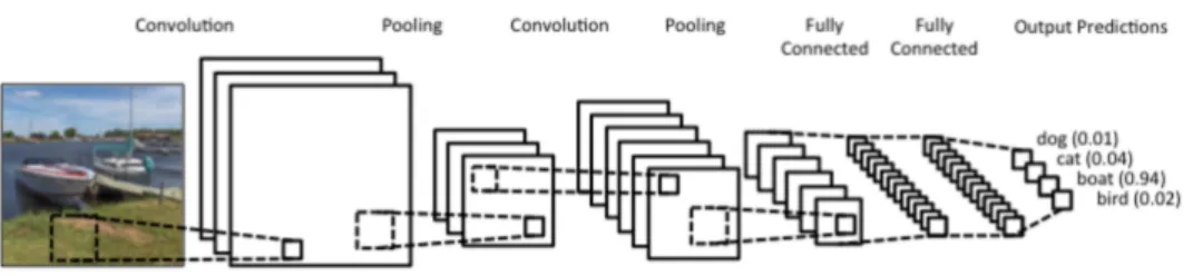
Figure 2.5: Basic convolutional neural network structure. Source:

http://www.wildml.com/2015/11/

understanding-convolutional-neural-networks-for-nlp/

degree of spatial invariance. A CNN usually consists of two types of lay-ers: convolutional layers and subsampling layers [6], as shown in figure 2.5. Convolutional layers consist of multiple rectangular grids of neurons called “filters” or “kernels”. In layer l of the CNN, filterFlof dimensionMl×Nl is applied on input image x. The output ofith _{filter at position (}_{j, k}₎ _Yl

ijk can be obtained by: Y_ijkl = Cl−1−1 X c=0 Ml−1 X a=0 Nl−1 X b=0 ficabxl_c,j−1−a,k−b (2.1) where there are Cl−1 channels in the (l −1)th layer, and ficab is the filter parameter at position (a, b) connecting input channel cto output channel i. This is called a convolution. Filter parametersfab can be learned to represent the features of the image.

Compared to fully connected layers, in convolutional layers the features are extracted more effectively from a small local region of an image, due to the fact that nearby pixels are more highly correlated by nature. The same set of weights is shared over the entire input image, which allows spatial invariance because the same feature can be detected in different locations.

The subsampling layers, also called pooling layers, perform a local averag-ing or subsamplaverag-ing on the filtered result. The advantage of this operation is that by reducing the resolution of the feature map it reduces the sensitivity of the output to input shift, rotation and distortions.

(11)

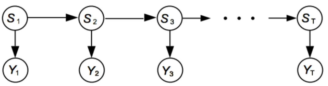
Figure 2.6: Hidden Markov model structure.

2.2 Model Development

2.2.1 Hidden Markov Models

Hidden Markov Models (HMMs) are very commonly used for modeling time series data [7]. HMM is a widely used stochastic model that represents the probability distribution over sequences of observations. The structure of an HMM is shown in figure 2.6. It has several underlying assumptions. First, the observation Yt at timet was generated by some process whose stateStis hidden. Second, the state of the process satisfies the Markov property: given the value of St−1, the currentSt is independent from all Sk wherek < t−1. Third, the hidden state variable St is discrete, and it only takes value from a set {1, . . . , K}.

By the Markov property, the joint distribution of a sequence of states and observations is specified by

P(S1:T, Y1:T) =P(S1)P(Y1|S1)ΠTt=2P(St|St−1)P(Yt|St) (2.2) Inference by HMMs starts with a prior distribution over model structures and parameters. A posterior probability distribution given the observation can be formed with Bayes rule, and the next observation can be inferred by calculating the predictive distribution. Model parameters of HMMs are obtained by the Expectation-Maximation (EM) algorithm, which adjusts the parameters to maximize the likelihood of the given dataset [7].

(12)

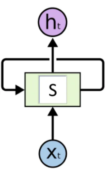
Figure 2.7: An RNN cell. Source:

http://colah.github.io/posts/2015-08-Understanding-LSTMs/

2.2.2 Recurrent Neural Network

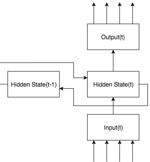
Artificial Neural Networks can significantly reduce the number of parameters when it comes to modeling language [8]. Given the fact that speech is a complex time-varying signal, Recurrent Neural Networks (RNNs) contain cyclic connections over time that make them a powerful tool to model such sequential data [9]. In figure 2.7, an arrow comes from S and goes back into

S shows the cyclic connection in each cell, and in figure 2.8, the recurrent connection in a RNN is shown briefly.

RNN hidden layer neurons hold a parameter called a “state”. The input vector x(t) to such cells is formed by the data d, and state at t−1.

x(t) =d(t) +s(t−1) (2.3)

sj(t) =f( X

i

xi(t)wji) (2.4)

where f is the sigmoid activation function

f(z) = 1

1 +e−z (2.5)

Output at layer L can be formulated as:

yL(t) =g( X

j

(13)

(14)

Figure 2.9: A single LSTM cell. Source: [12] where g is the softmax function

g(zi) =

ezi

P kezk

(2.7)

2.2.3 Long Short-Term Memory

Recurrent neural networks are trained by back-propagation through time [10]. In conventional RNNs, when the gradient of the error function is propagated back through the network, it gets scaled by a factor at each neuron, which is either greater than one or smaller than one. As a result, the gradient blows up or vanishes exponentially. This makes the training of such a network very difficult. To address this problem, Long Short-Term Memory (LSTM) structure is proposed [11], and has been applied on speech recognition and language modeling tasks [1].

The neuron cell in LSTM is designed to avoid the scaling effect. Instead of having a single set of weights from input to state, it adds a few gates to control the information flow. The mapping from input sequence xto output sequence h is calculated by:

(15)

it =σ(Wxixt+Whiht−1+Wcict−1+bi) (2.8) ft=σ(Wxfxt+Whfht−1+Wcfct−1+bf) (2.9) ot =σ(Wxoxt+Whoht−1+Wcoct+bo) (2.10) at=τ(Wxcxt+Whcht−1+bc) (2.11) ct=ftct−1+itat (2.12) ht=otθ(ct) (2.13) where σ is the sigmoid function,i, f, o, a, c are the input gate, forget gate, output gate, cell input activation, and the cell state respectively. Wci, Wcf and Wco are weight matrices for peephole connections [12], [13]. τ and θ are the cell input and cell output nonlinear activation functions. The connections are shown in figure 2.9.

The input gate in a cell is introduced to protect the memory content stored from irrelevant inputs. Likewise, the output gate is introduced to protect other cells from being interrupted by the currently irrelevant memory in this cell. The forget gate decides what information is kept in this cell.

Conventionally the LSTM cell only observes directly its cell output. Once the output gate is closed, the cell output will be close to zero. The peephole connection is designed to inspect the current cell state even when the output gate is closed [13]. The weights in the peephole connections are also updated by the error back-propagation rule.

A lot of variants from this LSTM architecture are derived. Architectures with no input gate, no output gate or no forget gate, etc. are experimented with on various datasets, and the most commonly used architecture described before performs reasonably well and no simple modification significantly im-proves the performance [14].

LSTM RNNs have been introduced to acoustic modeling and language modeling and achieve state-of-the-art performance. Experiments on LSTM lip reading have been done on small datasets to classify words [15]. There is also an LSTM-CNN hybrid audio-visual speech transcription system devel-oped that can beat a professional human lip reader [16].

(16)

CHAPTER 3 METHOD

3.1 The Audio-Visual Speech in a CAR (AVICAR)

Dataset

The AVICAR dataset is recorded in order to facilitate study of audio-visual speech recognition in a noisy environment [17]. The corpus is recorded in a car with different noise levels, and a large number of speakers comprised of 50 males and 50 females. The scripts they read consist of isolated digits, isolated letters, phone numbers and short sentences.

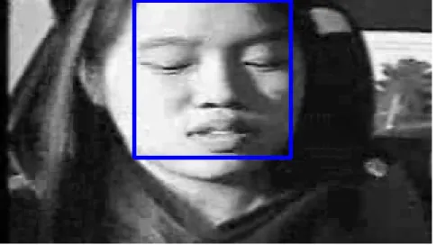
This study mainly uses the video data from this dataset. There are four cameras mounted on the corner of the windshield and dashboard, recording four synchronized video streams with slightly different views. The relative angle between the view and the speaker is unknown. A snapshot is shown in figure 3.1. The videos are recorded at 30 fps, with a resolution of 720×480 pixels.

The labels provided are the triphone state indexes every 10 milliseconds generated by an audio-only speech recognizer developed by other researchers. The indexes are in a range of [0,3896] and not necessarily linear, but it is observed that smaller labels around 40 refer to silent frames, and we label the indexes in the range [0,45] as silence.

3.2 Preprocessing Pipeline

Every frame extracted from the video is attached with a label. Since there are more labels than the frames, a timestamp for each frame is calculated and associated with the label with closest timestamp. While labeling the frames, a cascade classifier [9] is running to detect the face in the current frame, and

(17)

Figure 3.1: Gray-scale snapshot from the video.

the lower half of the face is cut out and kept to track the region of interest. Figure 3.2 shows the face detected in a snapshot. Figure 3.3 shows the lip region cut out from a detected face. We choose to detect faces instead of lips, since the view of the video data is slightly twisted, and the face detector achieves a far better accuracy than lip detectors in the experiments.

When loading the data, the image is resized to 40×80. Research has shown that the resolution does not affect the performance of automatic lip reading significantly [18], but it will affect the tracking process. So the images are only resized when they are fed to the neural network models.

3.3 Model Overview

Two models are constructed and trained. The first model consists of two convolutional layers as a feature extractor (see Appendix A.2, line 24-37), and two fully connected layers to perform the classification (see Appendix A.2, line 40-55), as in figure 3.4 (a). This model is trained with an error back-propagation algorithm.

The second one stacks two convolutional layers with one recurrent layer (see Appendix A.1), and a fully connected layer as the output layer. The

(18)

Figure 3.2: Detected face.

Figure 3.3: Resized lip region.

propagating the error back through the time axis as well, which is called back-propagation through time. This algorithm is implemented by unfolding the recurrent connections into a feed-forward structure as deep as the length of the sequence. The model structure is shown in figure 3.4 (b).

Four views are trained separately, and the output with highest probability is chosen to be the final class prediction of the current frame.

(19)

(a) (b)

(20)

CHAPTER 4 RESULTS

A total of 13950 training images are extracted from two speakers’ video files. A randomized 4/5 of the data is used for training, and the rest for testing. There are a total of 3897 triphone state indexes that are treated as labels. Due to lack of knowledge in linguistics, we do not have a correct method to group the indexes into clusters. The network is implemented in Python with Tensorflow [19], and trained to classify the training data into 3897 categories, or two categories, silence or speech.

The model in figure 3.4 (a) trained with two-class labels reaches 86.61% test set accuracy averaged across speakers, which shows that CNNs are capable of extracting lip features from various speakers. The confusion matrix in figure 4.1 shows that the predicted label is balanced throughout the test set. The 3897-class classification has an accuracy of 12.09% in test, which is reasonable because of the uneven distribution of the data, and the fact that the lip shapes in some classes are not clearly distinguishable.

The RNN/LSTM model, however, showed the behavior of getting stuck in local minima in both two-class and 3897-class training, even when the dataset has randomized order. Figure 4.2 (a) and (b) show that with the recurrent model, the training stops at a local minimum after a few epochs .

(21)

Figure 4.1: Confusion matrix for the two-class CNN.

(a) (b)

Figure 4.2: Convergence rate for the models, x-axis is epochs, y-axis is the sum of the average cost of each batch, where (a) is trained with 3897 classes and (b) is trained with 2 classes.

(22)

CHAPTER 5 DISCUSSION

Chapter 4 mentions that the recurrent network with either conventional RNN layer or LSTM layer converges to a local minimum. Specifically, the model learns to categorize input images into one of the categories regardless. Figure 5.1 (a) and (b) shows the confusion matrix of the test set for the model with conventional RNN layer after the first and the tenth epoch respectively. After 10 epochs, the model labels every test image as speech.

(a) (b)

Figure 5.1: Training results. (a) The confusion matrix after the first epoch and (b) the confusion matrix after the tenth epoch.

This could possibly because the silence vs. speech problem solely relying on visual information has more randomness than this network can model. Intuitively there is usually a silent period between two words, but the lip shapes at the beginning and the end of a word vary, and the sequential relationship between them is random. A model with deeper structures [6] trained with a larger amount of data might be able to learn the sequential relationship better.

Studies show that a deeper network with different structures shown in figure 5.2, such as stacking LSTM layers, or combining LSTM layers with

(23)

feed-forward layers can achieve a better performance than a single LSTM [12].

Figure 5.2: Examples of other LSTM structures. (a) A conventional LSTM, (b) an LSTM with input projection, (c) an LSTM with output projection, (d) an LSTM with deep input-to-hidden functions, (e) an LSTM with deep hidden-to-output functions and (f) stacked LSTMs. Source: [12]

(24)

CHAPTER 6 CONCLUSION

In this thesis, we reviewed a variety of approaches to perform lipreading, including stochastic methods and neural network methods, and experimented with a neural lipreading system utilizing a CNN and recurrent structure.

The result shows that, compared to traditional methods, a CNN feature extractor can capture the lip feature without an explicit lip shape model, and can tolerate some degrees of image variation and different lip shapes, which makes it a lot more generalizable.

The recurrent LSTM structure on the other hand, did not work out in the experiments. It echoes the acknowledged fact that recurrent neural networks are difficult to train. Future work might test improvements to the model, such as building a deeper network or combining it with other types of neural network structures.

(25)

APPENDIX A

PYTHON CODE

The code listed here is created with Tensorflow [19] and Numpy [20].

A.1 The Code for the RNN Layer

1 import numpy a s np

2 import t e n s o r f l o w a s t f

3 from t e n s o r f l o w . python . ops import rnn , r n n c e l l 4 5 def RNNlayer ( x , w e i g h t s , b i a s e s , b a t c h s i z e , i n p u t s i z e , s t e p s , h i d d e n s i z e , o p t i o n ) : 6 x = t f . r e s h a p e ( x , [−1 , i n p u t s i z e ] ) # b a t c h s i z e ∗ s t e p x i n p u t s i z e 7 x i n = t f . matmul ( x , w e i g h t s [ ’ i n ’ ] ) + b i a s e s [ ’ i n ’ ] 8 x i n = t f . r e s h a p e ( x i n , [−1 , s t e p s , h i d d e n s i z e ] ) 9 10 i f o p t i o n == ’ rnn ’ : 11 c e l l = r n n c e l l . BasicRNNCell ( h i d d e n s i z e ) 12 e l i f o p t i o n == ’ l s t m ’ : 13 c e l l = r n n c e l l . BasicLSTMCell ( h i d d e n s i z e , s t a t e i s t u p l e =True ) 14 15 i n i t s t a t e = c e l l . z e r o s t a t e ( b a t c h s i z e , dtype=t f . f l o a t 3 2 ) 16 output , f i n a l s t a t e = t f . nn . dynamic rnn ( c e l l , x i n , i n i t i a l s t a t e = i n i t s t a t e ) 17 o u t p u t = t f . r e d u c e m e a n ( output , 1 ) 18 r e s u l t = t f . matmul ( output , w e i g h t s [ ’ o u t ’ ] ) + b i a s e s [ ’ o u t ’ ] 19 20 return r e s u l t

(26)

A.2 The Code for the Models

1 from u t i l s import l o a d d a t a

2 from rnn import RNNlayer

3 4 def w e i g h t v a r i a b l e ( shape , n ) : 5 i n i t i a l = t f . t r u n c a t e d n o r m a l ( shape , s t d d e v = 0 . 1 ) 6 return t f . V a r i a b l e ( i n i t i a l , name=n ) 7 8 def b i a s v a r i a b l e ( shape , n ) : 9 i n i t i a l = t f . c o n s t a n t ( 0 . 1 , s h a p e=s h a p e ) 10 return t f . V a r i a b l e ( i n i t i a l , name=n ) 11 12 def conv2d ( x , W) :

13 return t f . nn . conv2d ( x , W, s t r i d e s = [ 1 , 1 , 1 , 1 ] , padding= ’SAME ’ ) 14

15 def m a x p o o l 2 x 2 ( x ) :

16 return t f . nn . max pool ( x , k s i z e = [ 1 , 2 , 2 , 1 ] , s t r i d e s = [ 1 , 2 , 2 , 1 ] , padding= ’SAME ’ )

17

18 def t r a i n c n n ( o p t i o n 1 , o p t i o n 2 , ma xla bel , n b a t c h e s ) : 19 x = t f . p l a c e h o l d e r ( t f . f l o a t 3 2 , s h a p e =[None , 4 0 , 8 0 , 1 ] ) 20 e l s e: 21 # y = t f . p l a c e h o l d e r ( t f . f l o a t 3 2 , s h a p e =[None , i n t ( m a x l a b e l ) +1]) 22 y = t f . p l a c e h o l d e r ( t f . f l o a t 3 2 , s h a p e =[None , 2 ] ) 23 24 w conv1 = w e i g h t v a r i a b l e ( [ 5 , 5 , 1 , 3 2 ] , ’ w conv1 ’ ) 25 b c o n v 1 = b i a s v a r i a b l e ( [ 3 2 ] , ’ b c o n v 1 ’ ) 26 w t r a n s p o s e d = t f . t r a n s p o s e ( w conv1 , [ 3 , 0 , 1 , 2 ] ) 27 28 h c o n v 1 = t f . nn . r e l u ( conv2d ( x , w conv1 )+ b c o n v 1 ) 29 h p o o l 1 = m a x p o o l 2 x 2 ( h c o n v 1 ) 30 31 w conv2 = w e i g h t v a r i a b l e ( [ 3 , 3 , 3 2 , 6 4 ] , ’ w conv2 ’ ) 32 b c o n v 2 = b i a s v a r i a b l e ( [ 6 4 ] , ’ b c o n v 2 ’ ) 33 34 h c o n v 2 = t f . nn . r e l u ( conv2d ( h p o o l 1 , w conv2 ) + b c o n v 2 ) 35 h p o o l 2 = m a x p o o l 2 x 2 ( h c o n v 2 ) 36 37 h p o o l 2 f l a t = t f . r e s h a p e ( h p o o l 2 , [−1 , 2 0∗1 0∗6 4 ] )

(27)

38 i f o p t i o n 2 == 0 : 39 # c l a s s i f i c a t i o n , one more r e a d o u t l a y e r 40 w f c 1 = w e i g h t v a r i a b l e ( [ 2 0∗1 0∗6 4 , 1 0 2 4 ] , ’ w f c 1 ’ ) 41 b f c 1 = b i a s v a r i a b l e ( [ 1 0 2 4 ] , ’ b f c 1 ’ ) 42 h f c 1 = t f . nn . r e l u ( t f . matmul ( h p o o l 2 f l a t , w f c 1 )+b f c 1 ) 43 44 h f c 1 d r o p = t f . p l a c e h o l d e r ( t f . f l o a t 3 2 , [ None , 1 0 2 4 ] , ’ h f c 1 d r o p ’ ) 45 46 k e e p p r o b = t f . p l a c e h o l d e r ( t f . f l o a t 3 2 , name= ’ k e e p p r o b ’ ) 47 h f c 1 d r o p = t f . nn . d r o p o u t ( h f c 1 , k e e p p r o b ) 48 49 # w f c 2 = w e i g h t v a r i a b l e ( [ 1 0 2 4 , i n t ( m a x l a b e l ) + 1 ] , ’ w f c 2 ’ ) 50 # b f c 2 = b i a s v a r i a b l e ( [ i n t ( m a x l a b e l ) + 1 ] , ’ b f c 2 ’ ) 51 52 w f c 2 = w e i g h t v a r i a b l e ( [ 1 0 2 4 , 2 ] , ’ w f c 2 ’ ) 53 b f c 2 = b i a s v a r i a b l e ( [ 2 ] , ’ b f c 2 ’ ) 54 55 y f c 2 = t f . matmul ( h f c 1 d r o p , w f c 2 ) + b f c 2 56 57 c r o s s e n t r o p y = t f . r e d u c e m e a n ( t f . nn . s o f t m a x c r o s s e n t r o p y w i t h l o g i t s ( y f c 2 , y ) ) 58 t r a i n s t e p = t f . t r a i n . AdamOptimizer ( 0 . 0 0 1 ) . m i n i m i z e ( c r o s s e n t r o p y ) 59 60 c o r r e c t p r e d i c t i o n = t f . e q u a l ( t f . argmax ( y f c 2 , 1 ) , t f . argmax ( y , 1 ) ) 61 a c c u r a c y = t f . r e d u c e m e a n ( t f . c a s t ( c o r r e c t p r e d i c t i o n , t f . f l o a t 3 2 ) ) 62 63 c o n v e r g e n c e = [ ] 64 65 i n i t = t f . i n i t i a l i z e a l l v a r i a b l e s ( ) 66 w i t h t f . S e s s i o n ( ) a s s e s s : 67 s e s s . run ( i n i t ) 68 69 f o r i in range( i t e r s ) : 70 c o s t = [ ] 71 f o r j in range( n b a t c h e s ) : ∗

(28)

73 i f len( x t )== 0 : 74 continue 75 , c u r r c o s t= s e s s . run ( [ t r a i n s t e p , c r o s s e n t r o p y ] , f e e d d i c t = {x : xt , y : yt , k e e p p r o b : 0 . 5}) 76 77 c o s t . append ( c u r r c o s t ) 78 79 i t e r c o s t = np .sum( np . a s a r r a y ( c o s t ) ) 80 print i t e r c o s t 81 82 c o n v e r g e n c e . append ( i t e r c o s t ) 83 84 f i l t e r s = w t r a n s p o s e d .eval( ) 85 x t e s t , y t e s t = l o a d d a t a ( 0 , 0 , i n t( m a x l a b e l ) , o p t i o n 1 , o p t i o n 2 , ’ t e s t ’ , 0 ) 86 t e s t a c c , p r e d i c t e d y= s e s s . run ( [ a c c u r a c y , y f c 2 ] , f e e d d i c t = {x : x t e s t , y : y t e s t , k e e p p r o b : 1 . 0}) 87 print ” t e s t s e t a c c u r a c y = ” , t e s t a c c 88 89 e l i f o p t i o n 2 == 3 : 90 # f u l l y c o n n e c t e d l a y e r a s t h e i n p u t o f rnn c e l l 91 w f c 1 = w e i g h t v a r i a b l e ( [ 2 0∗1 0∗6 4 , 1 0 2 4 ] , ’ w f c 1 ’ ) 92 b f c 1 = b i a s v a r i a b l e ( [ 1 0 2 4 ] , ’ b f c 1 ’ ) 93 h f c 1 = t f . nn . r e l u ( t f . matmul ( h p o o l 2 f l a t , w f c 1 )+b f c 1 ) 94 95 k e e p p r o b = t f . p l a c e h o l d e r ( t f . f l o a t 3 2 ) 96 h f c 1 d r o p = t f . nn . d r o p o u t ( h f c 1 , k e e p p r o b ) 97 98 l a y e r o p t i o n = ’ l s t m ’ 99 i n p u t s i z e = 1024 100 101 l t r a i n = t r a i n l e n g t h∗1 . 0 / b a t c h s i z e 102 l t e s t = t e s t l e n g t h∗1 . 0 / b a t c h s i z e 103 104 h f c 1 r e s h a p e d = t f . r e s h a p e ( h f c 1 d r o p , [−1 , s t e p s , i n p u t s i z e ] ) # r e s h a p e t o b a t c h s i z e , s t e p s , 1024 105 106 r n n w e i g h t s ={ 107 ’ i n ’ : t f . V a r i a b l e ( t f . random normal ( [ 1 0 2 4 , r n n h i d d e n ] ) ) , 108 ’ o u t ’ : t f . V a r i a b l e ( t f . random normal ( [ r n n h i d d e n , 2 ] ) ) 109 } 110 r n n b i a s e s ={

(29)

111 ’ i n ’ : t f . V a r i a b l e ( t f . o n e s ( [ r n n h i d d e n , ] ) ) , 112 ’ o u t ’ : t f . V a r i a b l e ( t f . o n e s ( [ 2 , ] ) ) 113 } 114 115 y r n n = RNNlayer ( h f c 1 r e s h a p e d , r n n w e i g h t s , r n n b i a s e s , b a t c h s i z e , i n p u t s i z e , s t e p s , r n n h i d d e n , l a y e r o p t i o n ) 116 117 i f y r n n == None : 118 print ” s t h wrong i n l s t m ” 119 s y s . e x i t ( ) 120 121 c r o s s e n t r o p y = t f . r e d u c e m e a n ( t f . nn . s o f t m a x c r o s s e n t r o p y w i t h l o g i t s ( y rnn , y ) ) 122 t r a i n s t e p = t f . t r a i n . AdamOptimizer ( 0 . 0 0 1 ) . m i n i m i z e ( c r o s s e n t r o p y ) 123 124 c o r r e c t p r e d i c t i o n = t f . e q u a l ( t f . argmax ( y rnn , 1 ) , t f . argmax ( y , 1 ) ) 125 a c c u r a c y = t f . r e d u c e m e a n ( t f . c a s t ( c o r r e c t p r e d i c t i o n , t f . f l o a t 3 2 ) ) 126 127 c o n v e r g e n c e = [ ] 128 i n i t = t f . i n i t i a l i z e a l l v a r i a b l e s ( ) 129 w i t h t f . S e s s i o n ( ) a s s e s s : 130 s e s s . run ( i n i t ) 131 132 f o r i in range( i t e r s ) : 133 c o s t = [ ] 134 f o r j in range( n b a t c h e s ) : 135 xt , y t = l o a d d a t a ( j∗b a t c h s i z e , b a t c h s i z e , i n t( m a x l a b e l ) , o p t i o n 1 , o p t i o n 2 , ’ t r a i n ’ , 1 , s t e p s ) 136 i f len( x t )== 0 : 137 continue 138 e l i f len( x t ) != b a t c h s i z e∗s t e p s : 139 continue 140 , c u r r c o s t= s e s s . run ( [ t r a i n s t e p , c r o s s e n t r o p y ] , f e e d d i c t = {x : xt , y : yt , k e e p p r o b : 0 . 5})

(30)

144 i t e r c o s t = np .sum( np . a s a r r a y ( c o s t ) ) 145 print i t e r c o s t 146 147 c o n v e r g e n c e . append ( i t e r c o s t ) 148 149 f i l t e r s = w t r a n s p o s e d .eval( ) 150 151 t r a i n a c c = [ ] 152 f o r i in range(i n t( l t r a i n ) ) : 153 xt , y t = l o a d d a t a ( i∗b a t c h s i z e , b a t c h s i z e , i n t ( m a x l a b e l ) , o p t i o n 1 , o p t i o n 2 , ’ t r a i n ’ , 1 , s t e p s ) 154 i f len( x t )== 0 : 155 continue 156 e l i f len( x t ) != b a t c h s i z e∗s t e p s : 157 continue 158 159 c u r r a c c = s e s s . run ( a c c u r a c y , f e e d d i c t ={x : xt , y : yt , k e e p p r o b : 1 . 0}) 160 t r a i n a c c . append ( c u r r a c c ) 161 162 print( ’ t r a i n i n g a c c u r a c y = ’ ) , 163 print np . mean ( np . a s a r r a y ( t r a i n a c c ) ) 164 165 t e s t a c c = [ ] 166 p r e d i c t e d y = [ ] 167 y t e s t = [ ] 168 f o r i in range(i n t( l t e s t ) ) : 169 xt , y t = l o a d d a t a ( i∗b a t c h s i z e , b a t c h s i z e , i n t ( m a x l a b e l ) , o p t i o n 1 , o p t i o n 2 , ’ t e s t ’ , 1 , s t e p s ) 170 i f len( x t )== 0 : 171 continue 172 e l i f len( x t ) != b a t c h s i z e∗s t e p s : 173 continue 174 y t e s t += y t 175 t e s t a c c . append ( s e s s . run ( a c c u r a c y , f e e d d i c t ={x : xt , y : yt , k e e p p r o b : 1 . 0}) ) 176 i f i == 0 : 177 p r e d i c t e d y = s e s s . run ( y rnn , f e e d d i c t ={x : xt , y : yt , k e e p p r o b : 1 . 0}) 178 e l s e:

(31)

179 p r e d i c t e d y = np . c o n c a t e n a t e ( ( p r e d i c t e d y , s e s s . run ( y rnn , f e e d d i c t ={x : xt , y : yt , k e e p p r o b : 1 . 0}) ) , a x i s =0) 180 181 print ” t e s t s e t a c c u r a c y = ” , 182 print np . mean ( np . a s a r r a y ( t e s t a c c ) ) 183 184 return c o n v e r g e n c e , f i l t e r s , p r e d i c t e d y , y t e s t

(32)

REFERENCES

[1] H. Sak, A. W. Senior, and F. Beaufays, “Long short-term memory based recurrent neural network architectures for large vocabulary speech recognition,” CoRR, vol. abs/1402.1128, 2014. [Online]. Available: http://arxiv.org/abs/1402.1128

[2] I. Matthews, T. Cootes, J. A. Bangham, S. Cox, and R. Harvey, “Ex-traction of visual features for lipreading,”IEEE Transactions on Pattern Analysis and Machine Intelligence, vol. 24, pp. 198–213, 2002.

[3] M. Pards and A. Bonafonte, “Facial animation parameters extraction and expression detection using HMM,” in Imaging of the Signal Pro-cessing: Image Communication Journal, 2002, pp. 675–688.

[4] J. Luettin, N. A. Thacker, and S. W. Beet, “Visual speech recognition using active shape models and hidden Markov models,” in 1996 IEEE International Conference on Acoustics, Speech, and Signal Processing Conference Proceedings, vol. 2, May 1996, pp. 817–820.

[5] Y. Li, Y. Takashima, T. Takiguchi, and Y. Ariki, “Lip reading using a dynamic feature of lip images and convolutional neural networks,” in 2016 IEEE/ACIS 15th International Conference on Computer and Information Science (ICIS), June 2016, pp. 1–6.

[6] Y. Bengio, “Learning deep architectures for AI,” Foundations and Trends in Machine Learning, vol. 2, no. 1, pp. 1–127, 2009.

[7] Z. Ghahramani, Hidden Markov Models. River Edge, NJ, USA: World Scientific Publishing Co., Inc., 2002, ch. An Introduction to Hidden Markov Models and Bayesian Networks, pp. 9–42.

[8] Y. Bengio, R. Ducharme, P. Vincent, and C. Janvin, “A neural proba-bilistic language model,” J. Mach. Learn. Res., vol. 3, pp. 1137–1155, Mar. 2003.

[9] T. Mikolov, M. Karafit, L. Burget, J. Cernock, and S. Khudanpur, “Re-current neural network based language model,” in INTERSPEECH, T. Kobayashi, K. Hirose, and S. Nakamura, Eds. ISCA, 2010, pp. 1045–1048.

(33)

[10] P. Werbos, “Backpropagation through time: What does it do and how to do it,” in Proceedings of IEEE, vol. 78, no. 10, 1990, pp. 1550–1560. [11] S. Hochreiter and J. Schmidhuber, “Long short-term memory,” Neural

Comput., vol. 9, no. 8, pp. 1735–1780, Nov. 1997.

[12] X. Li and X. Wu, “Constructing long short-term memory based deep recurrent neural networks for large vocabulary speech recognition,”

CoRR, vol. abs/1410.4281, 2014. [Online]. Available: http://arxiv.org/ abs/1410.4281

[13] F. A. Gers, N. N. Schraudolph, and J. Schmidhuber, “Learning precise timing with LSTM recurrent networks,” J. Mach. Learn. Res., vol. 3, pp. 115–143, Mar. 2003.

[14] K. Greff, R. K. Srivastava, J. Koutn´ık, B. R. Steunebrink, and J. Schmidhuber, “LSTM: A search space odyssey,” CoRR, vol. abs/1503.04069, 2015. [Online]. Available: http://arxiv.org/abs/1503. 04069

[15] M. Wand, J. Koutn´ık, and J. Schmidhuber, “Lipreading with long short-term memory,” CoRR, vol. abs/1601.08188, 2016. [Online]. Available: http://arxiv.org/abs/1601.08188

[16] J. S. Chung, A. W. Senior, O. Vinyals, and A. Zisserman, “Lip reading sentences in the wild,” CoRR, vol. abs/1611.05358, 2016. [Online]. Available: http://arxiv.org/abs/1611.05358

[17] B. Lee, M. Hasegawa-Johnson, C. Goudeseune, S. Kamdar, S. Borys, M. Liu, and T. S. Huang, “Avicar: Audio-visual speech corpus in a car environment,” in INTERSPEECH. ISCA, 2004.

[18] H. L. Bear, R. Harvey, B. J. Theobald, and Y. Lan, “Resolution limits on visual speech recognition,” in 2014 IEEE International Conference on Image Processing (ICIP), Oct 2014, pp. 1371–1375.

[19] M. Abadi, A. Agarwal, P. Barham, E. Brevdo, Z. Chen, C. Citro, G. S. Corrado, A. Davis, J. Dean, M. Devin, S. Ghemawat, I. Goodfellow, A. Harp, G. Irving, M. Isard, Y. Jia, R. Jozefowicz, L. Kaiser, M. Kudlur, J. Levenberg, D. Man´e, R. Monga, S. Moore, D. Murray, C. Olah, M. Schuster, J. Shlens, B. Steiner, I. Sutskever, K. Talwar, P. Tucker, V. Vanhoucke, V. Vasudevan, F. Vi´egas, O. Vinyals, P. Warden, M. Wattenberg, M. Wicke, Y. Yu, and X. Zheng, “TensorFlow: Large-scale machine learning on heterogeneous systems,”

(34)

[20] S. v. d. Walt, S. C. Colbert, and G. Varoquaux, “The numpy array: A structure for efficient numerical computation,” Computing in Science and Engg., vol. 13, no. 2, pp. 22–30, Mar. 2011. [Online]. Available: http://dx.doi.org/10.1109/MCSE.2011.37