HAL Id: tel-02271840
https://tel.archives-ouvertes.fr/tel-02271840
Submitted on 27 Aug 2019HAL is a multi-disciplinary open access archive for the deposit and dissemination of sci-entific research documents, whether they are pub-lished or not. The documents may come from teaching and research institutions in France or abroad, or from public or private research centers.
L’archive ouverte pluridisciplinaire HAL, est destinée au dépôt et à la diffusion de documents scientifiques de niveau recherche, publiés ou non, émanant des établissements d’enseignement et de recherche français ou étrangers, des laboratoires publics ou privés.
networks
Melanie Ducoffe
To cite this version:
Melanie Ducoffe. Active learning and input space analysis for deep networks. Neural and Evolutionary Computing [cs.NE]. Université Côte d’Azur, 2018. English. �NNT : 2018AZUR4115�. �tel-02271840�
THÈSE DE DOCTORAT
Active Learning et Visualisation
des données d'apprentissage pour
les réseaux de neurones profonds
Mélanie Ducoffe
CNRS, Laboratoire I3S, Sophia-Antipolis
Devant le jury, composé de: Présentée en vue de l'obtention
du grade de docteur en Informatique de Université Côte d'Azur
Frederic PRECIOSO, Université Côte d'Azur Directeur
Dirigée par: Frederic Precioso Karim LOUNICI,Université Côte d'Azur Président Patrick PEREZ, VALEO Rapporteur Bjorn SCHULLER, University of Augsburg Rapporteur
Soutenue le : 12 Décembre 2018 Stéphane CANU,INSA Rouen Examinateur Jakob VERBEEK, INRIA Grenoble Examinateur
Active Learning et Visualisation
des données d'apprentissage pour
les réseaux de neurones profonds
Jury
Président du jury
• Karim LOUNICI, Université Côte d'Azur
Rapporteurs
• Patrick PEREZ, VALEO
• Bjorn SCHULLER, University of Augsburg
Examinateurs
• Stéphane CANU, INSA Rouen • Jakob VERBEEK, INRIA Grenoble
iii
Titre : Active Learning et Visualisation des données d'apprentissage
pour les Réseaux de Neurones Profonds
Résumé
Notre travail est présenté en trois parties indépendantes.
Tout d'abord, nous proposons trois heuristiques d'apprentissage actif pour les réseaux de neurones profonds :
• Nous mettons à l'échelle le `query by committee' , qui agrège la décision de
sélec-tionner ou non une donnée par le vote d'un comité. Pour se faire nous formons le comité à l'aide de diérents masque de dropout.
• Un autre travail se base sur la distance des exemples à la marge. Nous proposons
d'utiliser les exemples adversaires comme une approximation de la dite distance. Nous démontrons également des bornes de convergence de notre méthode dans le cas de réseaux linéaires.
• Puis, nous avons formulé une heuristique d'apprentissage actif qui s'adapte tant
au CNNs qu'aux RNNs. Notre méthode sélectionne les données qui minimisent l'énergie libre variationnelle.
Dans un second temps, nous nous sommes concentrés sur la distance de Wasser-stein. Nous projetons les distributions dans un espace où la distance euclidienne mimique la distance de Wasserstein. Pour se faire nous utilisons une architecture siamoise. Également, nous démontrons les propriétés sous-modulaires des proto-types de Wasserstein et comment les appliquer à l'apprentissage actif.
Enn, nous proposons de nouveaux outils de visualisation pour expliquer les prédictions d'un CNN sur du langage naturel. Premièrement, nous détournons une stratégie d'apprentissage actif pour confronter la pertinence des phrases sélection-nées aux techniques de phraséologie les plus récentes. Deuxièmement, nous protons des algorithmes de déconvolution des CNNs an de présenter une nouvelle perspec-tive sur l'analyse d'un texte.
Mots clés
Apprentissage Actif, Wasserstein, Linguistique, Réseaux de neurones profonds, Dé-convolution, Automatisation, Exemple Adversaire
Title : Active Learning and Input Space Analysis for Deep
Networks
Abstract
Our work is presented in three separate parts which can be read independently. Firstly we propose three active learning heuristics that scale to deep neural net-works:
• We scale query by committee, an ensemble active learning methods. We speed
up the computation time by sampling a committee of deep networks by applying dropout on the trained model.
• Another direction was margin-based active learning. We propose to use an
ad-versarial perturbation to measure the distance to the margin. We also establish theoretical bounds on the convergence of our Adversarial Active Learning strategy for linear classiers.
• We also derive an active learning heuristic that scales to both CNN and RNN by
selecting the unlabeled data that minimize the variational free energy.
Secondly, we focus our work on how to fasten the computation of Wasserstein distances. We propose to approximate Wasserstein distances using a Siamese archi-tecture. From another point of view, we demonstrate the submodular properties of Wasserstein medoids and how to apply it in active learning.
Eventually, we provide new visualization tools for explaining the predictions of CNN on a text. First, we hijack an active learning strategy to confront the relevance of the sentences selected with active learning to state-of-the-art phraseology tech-niques. These works help to understand the hierarchy of the linguistic knowledge acquired during the training of CNNs on NLP tasks. Secondly, we take advantage of deconvolution networks for image analysis to present a new perspective on text analysis to the linguistic community that we call Text Deconvolution Saliency. Keywords
Deep Learning, Active Learning, Wasserstein, Linguistic, NLP, CNN, Deconvolu-tion, Adversarial example
v
Remerciements
Je remercie d'abord les membres de mon jury de thèse. Un grand merci en parti-culier à Patrick Perez et Björn Schuller pour avoir accepté de rapporter ma thèse. Mais également je remercie tous les membres du jury, Karim Lounici, Stéphane Canu, et Jakob Verbeek. C'est un honneur pour moi de présenter mes travaux devant des chercheurs dont l'excellence de leur recherche, mais également leur bi-enveillance ont été des sources d'inspirations durant mes trois années de doctorat. Je n'oublie pas également d'adresser un grand merci à Igor Litovsky, Johnny Bond et Christophe Papazian qui furent les premiers à me pousser vers la recherche. Je remercie également l'ENS Cachan-Rennes et les directeurs de leur département in-formatique, David Pichardie et Luc Bougé qui ont permis le nancement de cette thèse. Mes remerciements vont de même à Nicolas Nisse, Rémi Gribonval, Anatole Lécuyer et Yoshua Bengio pour m'avoir encadré dans mes stages de recherche. Dans ce contexte, je remercie tout particulièrement Yoshua Bengio et Pascal Vincent, pro-fesseur au MILA pour m'avoir enseignée énormément de concepts sur l'apprentissage automatique. Si je suis capable aujourd'hui de soutenir ma thèse, c'est en partie grâce à ce que j'ai appris à leurs côtés.
Un très grand merci du fond du c÷ur à mon encadrant, Frédéric Precioso, pour m'avoir fait conance. Merci à toi pour t'être toujours rendu disponible malgré un emploi du temps plus que chargé et pour tes conseils judicieux, tant humains que sci-entiques. Merci également pour les nombreuses opportunités auxquels tu m'as fait accéder. Aucun remerciement ne pourra correctement exprimer ma reconnaissance pour ton investissement.
Merci aux collaborateurs de cette thèse, en particulier, Rémi Flamary, Nicolas Courty, Damon Mayare et Laurent Vanni. Rémi a été la plus belle rencontre que j'ai pu faire pendant cette thèse. Il a choisi de me faire conance et de m'enseigner tout un pan du machine learning qui m'était alors inconnu. Toi et Nicolas êtes deux chercheurs et deux mentors incroyables, et je croise les doigts pour que dans l'avenir nous puissions encore travailler ensemble ! Damon, je n'aurais jamais une prose aussi élaborée que la tienne pour te remercier, mais le c÷ur y est. Collaborer avec toi et Laurent fût extrêmement enrichissant, et j'espère pouvoir continuer à travailler dans l'interdisciplinarité avec vous deux et Frédéric.
De manière plus indirecte, je tiens à remercier Mireille Borne-fontaine, Lucile Sassatelli, Diane Lingrand, Anne-Marie Pinna-Dery, Asja Fischer, Samira Shaba-nian, Negar Rostamzadeh et Joëlle Pineau. Être une femme dans un milieu majori-tairement composé d'hommes n'est jamais quelque chose d'aisé, et certaines anec-dotes à ce sujet auraient pu me détourner de ce milieu si jamais je n'avais pu me rassurer par votre réussite professionnelle et votre persévérance à contrer les ten-dances. Telle n'était pas votre intention, mais vous m'avez servi de modèles et je vous en remercie.
Que serait une thèse académique sans les collègues doctorants et chercheurs dont la gentillesse et la bonhomie ont largement contribué à me faire garder le sourire. En toute honnêteté, je devrais aussi remercier les producteurs de café et
de sucreries qui furent ma principale source d'alimentation. Je remercie mes co-bureaux: Xheva, qui m'a accueilli avec joie en pleine rédaction de thèse, puis Melissa qui a fait passer les heures de travail plus vite grâce à nos discussions. Merci au trio infernal Romaric, Yoann et Stéphanie, les irréductibles de la pause-déjeuner et la pause goûter, mais également à tous ceux qui m'ont tenu compagnie quand je pointais le bout de mon nez hors du bureau: Georey, Gérald, Thomas, Franck(s), Ben, Philippe(s), Stéphane, Jean-Yves, Anne Marie, Marco, Sébastien, Sami, Mehdi, Claude, Hélène, et à tous les autres que j'aurai oublié de mentionner. . . Merci à Ali Beikbaghban qui depuis mon entrée à Polytech a toujours été bienveillant avec moi et le reste de la tribu Ducoe. Je remercie également la merveilleuse Magali Richir, qui m'a toujours aidé avec diligence et gentillesse dans l'enfer administratif qui pave la vie d'un doctorant. Merci également aux collègues étrangers - entre autres Chiheb Trabelsi, Thomas Mesnard, Guillaume Alain, Benjamin Scellier - dont les rencontres annuelles aux conférences et écoles d'été m'ont fourni une motivation supplémentaire pour mes publications. Des remerciements particuliers à Christelle et Denis, mes `parents adoptifs'. Même si cette expression relevait avant tout de la blague, vous êtes un couple merveilleux et très attachant, je n'aurai pas été peu ère d'avoir fait partie de votre famille. De manière plus générale, je remercie tous les membres de l'équipe SPARKS. Merci à tous pour les moments de joie, de partage et de complicité !
Parmi les supers enseignants avec qui j'ai eu la chance de travailler, je remercie tout particulièrement Diane Lingrand. Merci à toi pour ton implication et ta con-sidération, mais aussi pour avoir su allier travail et humour. Travailler à tes côtés fut extrêmement gratiant d'un point de vue professionnel, mais aussi personnel.
Un immense merci à mes proches pour leur aection et leur soutien indéfectible. Des remerciements très spéciaux à mon frère et ma soeur, Guillaume et Anaïs, avec qui j'ai la chance d'être très proches, et qui m'ont notamment consolée après les rebuttals diciles. Vous êtes les meilleurs frères et soeurs qu'on puisse avoir ! Guillaume, tu as été un moteur pendant cette thèse, ta passion pour la science et ton acharnement m'ont toujours poussé à donner le meilleur de moi-même. J'espère un jour être à ta hauteur ! Merci à Clément pour m'avoir fait réaliser que je n'étais pas mariée à ma thèse, et que la passion de la recherche n'est rien sans une vie personnelle épanouissante. Je souhaite qu'elle le soit longtemps à tes côtés. Je remercie également ma soeur de coeur Félicia, et mes amis proches Emilie, Axelle, Marie, Laura, Arnaud, Raphaël et Claudia pour avoir toujours cru en moi. Un grand merci au duo de choc Heck, David et Jonathan, pour leur humour et pour avoir introduit les soirées jeux. Obéron a tenu trois ans en thèse grâce à vous ! Merci à Jipsy, ma bouillotte personnelle qui dort tous les soirs sur mes jambes, et pour tous les ronronnements de mes chats, Mistoue, Pelote, Kiki et Lolita. Merci bien sûr à mes parents, Dominique et Evelyne. Je n'ai réalisé que trop tardivement les sacrices et les concessions que vous avez faits pour nos avenirs. Je ne mérite rien que vous ne m'ayez appris ou oert et je vous suis reconnaissante pour tout ce que vous avez fait pour moi. Enn je fais un merci général à ma grand-mère, à ma belle-soeur Adriana, ainsi qu'au reste de mes amis et de ma famille.
vii De manière plus anecdotique, je remercie Cédric Villani dont les actions poli-tiques cherchent à pérenniser l'avenir de l'apprentissage articiel en France. J'aime mon pays et je suis heureuse de voir émerger de nouvelles opportunités qui me permettent de rester.
Contents
1 Introduction 1
1.1 Contributions . . . 1
1.1.1 Active Learning for Deep Networks . . . 1
1.1.2 Learning Wasserstein Core-Sets . . . 2
1.1.3 Visualization and Active Analysis for Deep Networks on Lin-guistic tasks. . . 2
1.2 List of publications . . . 2
I Active Learning for Deep Networks 5 2 Introduction 7 2.1 Motivations . . . 7
2.2 Denitions . . . 8
2.2.1 Active Learning . . . 8
2.2.2 Related Research Areas . . . 11
2.3 Litterature . . . 12
2.3.1 Uncertainty . . . 12
2.3.2 Query-By-Committee . . . 13
2.3.3 Optimal Experimental Design . . . 13
2.3.4 Core-Set . . . 15
2.3.5 Expected Model Change . . . 15
2.3.6 Batch Active Learning . . . 17
2.4 Theoretical Justication of Active Learning for Deep Networks . . . 18
3 Dropout Query-By-Committee 23 3.1 Introduction . . . 23
3.2 Sampling a committee with Dropout . . . 25
3.3 Disagreement Scoring Function . . . 27
3.4 Empirical Validation . . . 28
3.5 Conclusion. . . 29
4 Adversarial Active Learning 31 4.1 Introduction . . . 32
4.2 Margin-Based Active Learning for Deep Networks . . . 34
4.3 Empirical Validation . . . 36
4.3.1 Dataset and hyperparameters . . . 36
4.3.2 Evaluation. . . 37
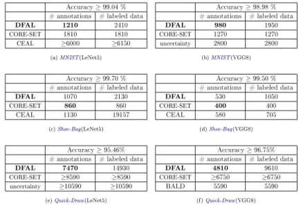
4.3.3 Comparative study between DFAL and CORE-SET . . . 40
4.5 Discussion . . . 44
4.5.1 Theoretical motivations . . . 44
4.5.2 DFAL does not select random samples in the rst runs . . . . 44
4.6 Adversarial Active Learning for Linear Classiers . . . 46
4.6.1 Transferable adversarial attacks . . . 46
4.6.2 Label Complexity on the unit ball . . . 49
4.7 Conclusion. . . 50
5 Perspective: Bayesian Active Learning through Laplace Approxi-mation 51 5.1 Introduction . . . 51
5.1.1 Active Learning under the light of Variational Inference . . . 53
5.2 Covering . . . 56
5.2.1 Optimal Experimental Design . . . 56
5.2.2 Increasing the diversity . . . 57
5.3 Application to CNN . . . 58 5.4 Application to RNN . . . 59 5.5 Empirical Validation . . . 61 5.6 Future work . . . 63 5.7 Conclusion. . . 64 6 Conclusion 65 II Learning Wasserstein Core-Sets 67 7 Introduction 69 7.1 Motivations . . . 69
7.2 Denitions. . . 70
7.3 Litterature . . . 71
7.3.1 Fast approximation of the exact Wasserstein distance . . . 71
7.3.2 Metric embedding . . . 73
7.3.3 Domain adaptation . . . 73
7.3.4 Wasserstein Core-Sets for Lipschitz Costs . . . 74
7.3.5 Herding . . . 75
8 Learning Wasserstein embeddings 77 8.1 Introduction . . . 77
8.2 Wasserstein learning and reconstruction with siamese networks . . . 78
8.3 Empirical Validation . . . 80
8.3.1 Wasserstein data mining in the embedded space . . . 82
8.4 Future work: Wasserstein for Text Mining . . . 87
8.4.1 Information Retrieval: Fast computing of WMD at large scale 88 8.4.2 Text Generation given Wasserstein Distance . . . 90
Contents xi
9 Perspective: Wasserstein prototypes 95
9.1 Introduction . . . 95
9.2 Approximate Submodularity for Wasserstein distance . . . 96
9.2.1 Greedy selection of Prototypes . . . 98
9.3 Empirical Validation . . . 99
9.4 Active Learning . . . 102
9.5 Conclusion. . . 103
10 Conclusion 105 III Understanding the behavior of Neural Networks on Linguis-tic tasks 107 11 Introduction 109 11.1 Motivation. . . 109
11.2 Litterature . . . 110
11.2.1 CNNs for Text classication . . . 110
11.2.2 Visualization of Deep network. . . 111
11.2.3 Model Agnostic Explanation. . . 112
11.2.4 Adversarial example for NLP . . . 112
12 Deconvolution for Text Analysis 115 12.1 Introduction . . . 115
12.2 CNNs for Text Classication . . . 116
12.3 Deconvolution . . . 117
12.4 Experiments . . . 118
12.5 Z-score Versus Activation-score . . . 118
12.5.1 Dataset: English . . . 120
12.5.2 Dataset: French. . . 121
12.5.3 Dataset: Latin . . . 123
12.6 Conclusion. . . 125
13 Perspective: Active Learning for Linguistic Analysis 127 13.1 Introduction . . . 127
13.2 Methodology . . . 128
13.3 Analysis under the light of Phraseology expertise . . . 129
13.4 Future works: Analysis with Model Agnostic Explanations . . . 131
13.5 Conclusion. . . 131
14 Conclusion 133 IV Conclusion 135 14.1 Perspectives . . . 137
14.2 Conclusion. . . 137
A Appendix 147 A.1 Dataset . . . 148
A.2 Hyperparameters . . . 151
A.2.1 Dropout Query-By-Committee . . . 151
A.2.2 Adversarial Active Learning . . . 151
A.2.3 Bayesian Active Learning through Laplace Approximation . . 152
A.2.4 Learning Wasserstein embeddings . . . 152
A.2.5 Deconvolution for Text Analysis . . . 153
A.3 Proofs . . . 154
A.3.1 Adversarial Active Learning . . . 154
A.3.2 Bayesian Active Learning through Laplace Approximation . . 157
A.3.3 Monotony . . . 158
A.3.4 Wasserstein prototypes . . . 160
Chapter 1
Introduction
Contents1.1 Contributions . . . 1
1.1.1 Active Learning for Deep Networks . . . 1
1.1.2 Learning Wasserstein Core-Sets . . . 2
1.1.3 Visualization and Active Analysis for Deep Networks on Lin-guistic tasks. . . 2
1.2 List of publications . . . 2
1.1 Contributions
Our work is presented in three separate parts which can be read independently. We present their content in Parts 1.1.1, 1.1.2, 1.1.3 respectively. For each topic, we dedicate a thorough introduction. Full papers and code can be found online1, and
are also referred in Section 1.2.
1.1.1 Active Learning for Deep Networks
Part I is adressing the question of the annotation cost when training deep neural networks. Considering the cost of gathering relevant annotations for huge datasets such as ImageNet, the interest in methods requiring smaller training sets is increas-ing. One possible direction to improve a training set while reducing its size is to rely on active learning. In active learning, the goal is to train a classier with as few as possible training samples while reaching the same accuracy as if an unlimited number of training samples were available (i.e., at most the whole dataset). The challenge lies in selecting a small subset of data, without supervision, which is in-formative enough to reach the best possible accuracy. In Sections 3 to 4, we scale active learning methods mostly designed forConvolutional Neural Network (CNN). First, active query strategies may be handled by ensembling deep networks; ei-ther by disagreement over the models (Query By Committee: [Ducoe 2015], Chap-ter3), or by assuming some weight's distribution and sample a committee according to this distribution (Bayesian Active Learning: [Ducoe 2016c], Chapter5).
Another direction is to rely on the distance to the decision boundary, namely margin-based active learning. In Chapter 4, we exploit the geometric distances of samples to the decision boundaries for querying new samples. We propose to use an adversarial perturbation to measure the distance to a CNN's decision boundary in [Ducoe 2018]. We also establish theoretical bounds on the convergence of our Adversarial Active Learning strategy for linear classiers.
1.1.2 Learning Wasserstein Core-Sets
Part II is focusing on Wasserstein distance. Wasserstein is a distance between dis-tributions derived from the eld of optimal transport. It has received a lot of attention in machine learning recently, notably with Wasserstein based generative models. However, its complexity limits the usage of Wasserstein in new applica-tions. To alleviate the cost of computing pairwise Wasserstein distance on discrete distributions, we propose in Chapter8to approximate Wasserstein distances using a Siamese architecture ([Courty 2017b]). From another point of view, we demonstrate the submodular properties of Wasserstein medoids in Chapter 9 and how to apply it in active learning in Section 5.2.
1.1.3 Visualization and Active Analysis for Deep Networks on Lin-guistic tasks
We dedicate PartIIIto the conception of new visualization tools for the underlying information captured by a CNNon a text.
First, we hijack our active learning strategy from Chapter3to confront the rel-evance of the sentences selected with active learning to state-of-the-art phraseology techniques [Ducoe 2016a,Mayare 2017]. These works help to understand the hi-erarchy of the linguistic knowledge acquired during the training ofCNNsonNatural Language Processing (NLP) tasks.
Secondly, [Vanni 2018] confronts Textual Data Analysis and Convolutional Neu-ral Networks for text analysis. We take advantage of deconvolution networks for image analysis to present a new perspective on text analysis to the linguistic com-munity that we call Text Deconvolution Saliency (TDS), in Chapter 12.
1.2 List of publications
1. QBDC: Query by dropout committee for training deep supervised architecture [Ducoe 2015]
2. Adversarial Active Learning for Deep Networks: a Margin Based Approach [Ducoe 2018]
1.2. List of publications 3 3. Learning Wasserstein Embeddings [Courty 2018]
4. Introducing Active Learning for CNN under the light of Variational Inference [Ducoe 2016c]
5. Machine Learning under the light of Phraseology expertise [Ducoe 2016a] 6. Textual Deconvolution Saliency (TDS): a deep tool box for
linguis-tic analysis [Vanni 2018]
7. Les mots des candidats, de allons à vertu [Mayare 2017]
8. Scalable batch mode Optimal Experimental Design for Deep Net-works [Ducoe 2016b]
Part I
Active Learning for Deep
Networks
Chapter 2
Introduction
Contents 2.1 Motivations . . . 7 2.2 Denitions. . . 8 2.2.1 Active Learning. . . 82.2.2 Related Research Areas . . . 11
2.3 Litterature . . . 12
2.3.1 Uncertainty . . . 12
2.3.2 Query-By-Committee . . . 13
2.3.3 Optimal Experimental Design . . . 13
2.3.4 Core-Set . . . 15
2.3.5 Expected Model Change . . . 15
2.3.6 Batch Active Learning . . . 17
2.4 Theoretical Justication of Active Learning for Deep Net-works. . . 18
2.1 Motivations
Larger deep architectures fed with more data provide better results in error rate. This widely acknowledged idea has been conrmed all along the recent years when analyzing, for instance, the results at Imagenet Large Scale Visual Recognition Challenge [Russakovsky 2015]. Indeed, in 2012, the winner was the SuperVision team [Krizhevsky 2012] using a deep convolutional neural network with 60 million parameters and making a momentous breakthrough in the image classication task. The huge step forward from SuperVision team has profoundly impacted the following contributions to ILSVRC after 2012. In 2014, Simonyan et al. [Simonyan 2014] also proposed to use a CNN architecture from 11 up to 19 layers with 133 up to 144 million of parameters. Owing to the considerable amount of parameters involved which needs to be learned, the training set needs to be huge as well. Nevertheless, state of the art results using deep networks are known on a large training set.
However, a lot of real-life scenarios typically do not come with millions of labeled data available to train a model. Labeling appears to be one of the main bottlenecks towards wide spreading deep networks to a new area: gathering and annotating
massive dataset for supervised learning may prohibit the expansion of deep networks towards new elds such as chemistry or medicine [Smith 2018,Hoi 2006].
Labeling data may sound like a trivial task, but in many cases, it requires expert knowledge. For example, the creation of the Penn Treebank dataset, a benchmark when considering part-of-speech tagging, took more than seven years of collabora-tions with linguistic experts [Taylor 2003]. Scaling the labeling process is not always practical as it requires the intervention of many specic human operators. Usually, labeling can only be solved with coee and patience.
A more plausible solution is to reduce the compelling need for labeled training samples to train deep networks. In Section2.2, we highlight the dierent families of methods seeking to solve this type of problem and detail the settings on which they are better suited. In particular, we will focus on Active Learning (AL) that seeks to optimize the training set automatically for the task at hand to limit the need for human annotations.
2.2 Denitions
2.2.1 Active Learning
Given a large set of unlabeled samples, AL tries to guess which ones should be labeled and added to the training set to increase at best the performance of your model. It operates iteratively, by rst requesting new labels from the user, and then updating the model given the new labeled training set. The model can leverage its new knowledge to add queries again. Eventually, only a small fraction of the unla-beled data would be annotated to achieve good classication performance. Firstly, we detail three scenarios in which may occur AL. Note that this list is not intended to be exhaustive. Eventually, AL may occur in dierent scenarios:
• Pool-Based Sampling assumes that the learner has only access to a xed
pool P of unlabeled i.i.d samples (C) and must query a xed budget size
number of points (D) fromP. It submits each of those queries to an oracle (E)
that labels them to add them into the labeled training set (A). The classier (B) can then be re-trained on the incremented labeled training set. Figure2.1
illustrates the iterative process. Notice that, in our context, we assume that the oracle makes no mistakes when annotating new query. However, noisy oracles have been tackled in the literature. For a survey of noisy oracles, we refer the reader to [Settles 2011].
• Stream-Based Selective Sampling considers one unlabeled example at a
time and for each of them decide whether to ignore it or ask an oracle to an-notate it. Stream-based active learning is attractive in many real-world appli-cations when unlabeled samples are presented sequentially, and their number is far too large to maintain a pool of candidates. For example, stream-based active learning may be suitable for the classication of observations by
au-2.2. Denitions 9 DOG PIG + (A) (B) (C) (D) (E)
Figure 2.1: Illustration of Pool-Based Active Learning: A=Labeled training set ; B=Classier ; C=Unlabeled set ; D=Queries ;E=Oracle
tonomous car driving.
• Query synthesis consists in generating new unlabeled instances instead of
considering a xed pool of unlabeled samples. Creating de novo the queries may increase the learning speed, as we can optimize the queries according to the query selection. We illustrate this phenomenon with a simple example in Figure2.2.
However querying arbitrary instances can be awkward if there are no assump-tions on the underlying distribution of the generated samples; in that case, we may generate noisy instances. For example, [Baum 1992] synthesized hand-written digits to train a neural network. However, they obtained poor per-formance as sometimes their generated queries were not identiable to the human oracle. Early active query synthesis has encountered some success when considering very low dimensional domains. More recently, [Zhu 2017] proposed to use a pre-trainedGenerative Adversarial Network (GAN)to gen-erate the queries. So far, they obtain competitive results with pool-based active learning, probably due to a lack of diversity in their criterion. Indeed, when sampling from a nite set, the optimization of the query selection crite-rion is limited by the number of samples and their distribution. Eventually, one should pay attention not to focus on a subregion of the underlying dis-tribution and create bias in the labeled training set. While their method is interesting, it comes at the price of training a GAN in a preprocessing step, which remains a challenging task. Nevertheless, query synthesis is also used as a form of reinforcement learning to improve dialogue generation: after the training phase, a human oracle scores the generated answer, which helps to
(a)SV Mactive (b) Query synthesis
Figure 2.2: An active learning heuristics for SVM SV Mactive will query data that
are the closest to the decision boundary. In that tendency, Query synthesis may help to generate queries that optimize the active learning criterion as underlined in2.2(b) [Zhu 2017]
improve the system in [Asghar 2017].
Active learning is not only motivated by theoretical works demonstrating that one model may perform better using less labeled data if the data are model-crafted [Cohn 1996], but also by its proven eciency on a wide range of machine learning procedures, including character recognition [Liu 2004], bio-informatics [Sculley 2007,
Smith 2010], or classication of medical data [Hoi 2006]. As an example, in Fig-ure2.3, we illustrate the potential benet of AL on a baby task.
A central challenge in active learning is to dene the information required for selecting at best the queries and how to measure it eectively. It happens that AL may have a drastic improvement regarding human annotations: in some classi-cation problems, the excess risk of AL can converge to zero with an exponential rate comparing with the linear rate of fully supervised classication, also known as passive learning. However, the eectiveness of AL implies prior knowledge on the data distribution [Willett 2006, Castro 2007]. Eventually, there exists no uni-versal criterion to select the most informative queries. Thus AL strategies rely on heuristics to choose these queries. Moreover, several heuristics coexist as it is im-possible to obtain a universal active learning strategy eective for any given task [Dasgupta 2005a].
As underlined in the related research areas2.2.2, applying active learning on deep networks appears promising. Indeed, in peculiar settings, supervised classication on random small labeled training set achieves similar accuracy than state-of-the-art semi-supervised deep algorithms. If one could optimize the labeled training set itself, it is likely that the performance would be even comparable, or even better.
2.2. Denitions 11 w positive examples negative examples A D C B
Figure 2.3: AL on a toy data-set. We consider a binary classication tasks on n=100 samples ( • positive examples, • negative examples) and want to learn an
optimal classier with no bias. Because the data are well separated, there exist an optimal linear classier (W) that can be learnt using at minima four samples: by labelling (A, B, C, D). However, the probability of sampling those points at once is of 1
(n
4)
'10−4
intuitive. First of all, scaling them to high dimensional parameters networks may turn out to be intractable: some classic active learning methods such as Optimal Experiment Design [Yu 2006] require to inverse the Hessian matrix of the models at each iteration, which would be intractable for current standardCNNs. Secondly, one of the most standard strategies is to rely on the uncertainty measure. Uncertainty in deep networks is usually evaluated through the network's output while this is known to be misleading. Indeed, the discovery of adversarial examples has demonstrated that the way we measure uncertainty may be overcondent. We describe the query selection methods proposed for deep networks in section2.3 and demonstrate how they compare to one another.
2.2.2 Related Research Areas
We dene close related research areas, relevant as well to reduce the eective size of the labeled training set to train deep models. While those topics are out of the scope of our work, they appear complementary to AL.
1. Transfer Learning (TL) consists in using a solution designed for a related source domain, in order to adapt it to the current problem. Usually, TL is used only when few samples from the target domain are available, a.k.a we do not have at our disposal a large set of unlabeled examples; which diers from AL. Nevertheless, TL is only applicable when both source and target domains share some relevant information; while dening the type of information required is not intuitive and typically induces several empirical experiments.
Transfer Learning is popular in deep learning due to a large number of pre-trained networks available online. When it comes to TL on deep networks,
it mainly consists in tting an already trained model to a new classication task on another dataset [Sawada 2017]. Indeed, it appears that deep neural networks trained on image classication tasks, all learn similar and broadly general features in their rst layers (visually similar to Gabor lters and color blobs, i.e., biologically receptive elds [Zamir 2018]). Hence, as those features are not dataset-crafted, they may be reused for another task to speed up the training: the scope of solutions would be narrowed by starting from a weight's region dierent from the common one obtained with random initialization. 2. Semi-Supervised Learning (SSL): combines both a small labeled training
set and a larger pool of unlabeled samples. When it comes to deep net-works, SSL enjoys an extensive literature, ranging from extending autoen-coders and generative modeling [Kingma 2014,Gogna 2016], to new regular-ization schemes [Miyato 2017]. Note that the previous listing is far from being exhaustive.
However, the new aws underlined in [Oliver 2018] should leverage the suc-cesses of semi-supervised deep algorithms. The rst drawback is that when us-ing well-optimized hyperparameters and regularization settus-ings, fully-supervised deep networks are competitive with the current state-of-the-art semi-supervised algorithms, without using any unlabeled samples. Nevertheless, the size of the labeled training set and also, the divergence between both distributions, respectively induced by the labeled samples and the unlabeled samples, pro-foundly impact the performance of SSL on classication tasks. Finally, both drawbacks highlight the necessity of optimizing the labeled training set for the task at hand.
2.3 Litterature
Previous works have shown that a carefully designed query strategy eectively re-duces annotation eort required in a variety of tasks for shallow models. The eec-tiveness of AL has been established both theoretically and empirically. Nevertheless, AL for shallow models mainly rely on specic model simplications and closed form solution. Deep Neural Networks, on another side, are inherently complex non-linear functions. Their complexity poses several limitations to scale such existing active learning strategies.
In this section, we establish the range of active learning methods studied for deep networks, starting from the most intuitive setup (uncertainty estimation) to the most sophisticated strategies that take into account some properties and specicities involved in the training of deep networks.
2.3.1 Uncertainty
Originally, [Lewis 1994] introduces uncertainty selection. It consists in querying the annotations for the unlabeled samples with the lowest condence. Thus its cost
2.3. Litterature 13 is low and its setup simple. Hence, it has been used on deep networks for various tasks, ranging from sentiment classication to visual question answering and Named Entity Recognition [Zhou 2010,Lin 2017a,Yanyao Shen 2018].
The main drawback of uncertainty selection is its tendency to query outliers or other types of noisy instances, such as adversarial examples. Tellingly, the apparition of adversarial attacks, which are wrongly predicted with high condence, empirically demonstrates that the probability of misclassication and the uncertainty are not necessarily correlated.
Uncertainty selection has been improved in a pseudo-labeling method called CEAL [Wang 2016]: CEAL performs uncertainty selection, but also adds highly condent samples into the augmented training set. The labels of these samples are not queried but inferred from the network's predictions. In the case one deals with a highly accurate network, CEAL will improve the generalization accuracy. However, CEAL implies new hyperparameters to threshold the prediction's condence. If such a threshold is poorly tuned, it will corrupt the training set with mistaken labels. 2.3.2 Query-By-Committee
Uncertainty selection may be also tailored to network ensemble, either by disagree-ment over the models (Query-by-committee, [Seung 1992]) or by sampling through the distribution of the weights (Bayesian active learning, [Kapoor 2007]). Query-by-Committee consists in maintaining a committee of models which represent the current set of consistent hypothesis. Whether to label or not a query is decided based on a vote among the committee members. Usually, the vote incorporates some disagreement information on the predicted labels. Figure 2.4 illustrates this process for linear classiers. Recently, [Gal 2016b] demonstrated that dropout (and other stochastic regularization schemes) is equivalent to perform inference on the posterior distribution of the weights, enabling to leverage the cost of training and updating multiple models. Thus, dropout allows to sample an ensemble of models at test time: to perform Dropout-Query-By-Committee (Ducoe et al. , [Ducoe 2015]) or Bayesian Active Learning (Gal et al. , [Gal 2016b]). Gal et al. proceeded with a comparison of several active learning heuristics: among all the metrics, BALD-which maximizes the mutual information between predictions and model posterior consistently outperforms other metrics.
2.3.3 Optimal Experimental Design
From another theoretical point of view, Optimal Experimental Design (OED) is a eld which takes interests in the Fisher information. Formally, the Fisher informa-tion is the expectainforma-tion over the partial derivative of the log-likelihood funcinforma-tion with respect to the parameters. The Fisher informations Ireads:
IΘ=Ex,y
∇Θl(fΘ(x), y)∇Θl(fΘ(x), y)T
(2.1) This measure is relevant because in a single parameter case, its inverse sets a
Figure 2.4: Version space example for linear classiers on a binary task. Every hypothesis () is consistent with the labeled training set. However, each of them represent a dierent model in the version space. The unlabeled sample in redis not relevant as a query because every classier agree in its prediction (it is a dog, whereas the green unlabeled sampleis interesting as it will shrink the number of consistent classiers. The more classiers we discard, the faster QBC converge towards the optimal classier for the task at hand (assuming that a linear classier can solve exactly the problem at hand)
lower bound on the variance of the model's parameter estimates; this result is known as the Cramer Rao bound [Kagan 2001,Kay 2013].
In other words, to minimize the variance over its parameter estimates, an active learner should select data that maximize the Fisher information or minimize the inverse.
But for multivariate parameters, the Fisher information is a covariance matrix, so its maximization may go through several statistics.
We cite the three most popular scenarios (other variants exist but, less used by the community, they are left unlisted for the sake of clarity):
• A-optimality minimizes the trace of the inverse information matrix [Chan 1982] • D-optimality minimizes the determinant of the inverse information matrix
[Chaloner 1995]
• E optimality minimizes the maximum eigenvalue of the information matrix
[Flaherty 2005]
Because deep neural networks may involve millions of parameters, computing their Fisher matrix is intractable. Moreover, even relying on approximations is too computationally expensive as one need to update the estimate for every possible query. Hence, OED has never been investigated for deep neural networks.
2.3. Litterature 15 2.3.4 Core-Set
[Ozan Sener 2018] dene the batch active learning problem as a covering problem on the output space of the network. In Equ.2.2, they minimize the population risk of a model learned on a small labeled subset. To do so, they propose an upper bound with a linear combination of the training error, the generalization error and a third term denoted as the core-set loss. Notice that in Equ. 2.2, we denote by s the set
of labeled points on which we train the parameterwof the network. We denote by
l(x, y|w,s) the loss of the network over a samplex with labely.
P opulation Risk ≤Generalization Error + T raining Error+ CoreSetLoss
Generalization Error≡Ex,y∼pZ[l(xi, yi|w,s)]−
1 n X i∈[n] l(xi, yi|w,s) T raining Error≡ 1 |s| X j∈s l(xj, yj |w,s) (2.2) The generalization error is the absolute dierence between the expectation of the loss considering every possible sample from the ground-truth distribution, and the expectation given the set of data available (meaning both labeled and unlabeled set, which are indexed by nin Equ.2.2). On another side, the training error measures
how far is the loss over both the unlabeled and labeled points compared to the loss evaluated only on the labeled points. Due to the expressive power of CNNs, the authors argue that the rst two terms (training and generalization error) are negligible. Therefore the population risk would mainly be controlled by the core-set loss. Given a labeled training set s, a model w trained ons, and an unlabeled set
of n points, the core-set loss is expressed in equation 2.3
CoreSetLoss≡ 1 n X i∈[n] l(xi, yi |w)− 1 |s| X j∈s l(xj, yj |w) (2.3)
The core-set loss consists in the dierence between the average empirical loss over the set of points which are already labeled, and the average empirical loss over the entire dataset including unlabeled points. If not considering the labels, the core-set loss is upper bounded with the covering radiusδs, as illustrated in Fig.2.5. Here, we
denote by covering radius, the maximum distance in the output space between any labeled sample's prediction and any unlabeled sample's prediction. Finally, Sener et al. used a MIP heuristic to minimize at best the covering radius of the training set. We illustrate their method in Fig.2.5(b). Thanks to their method, they achieve state-of-the-art performance in active learning for image classication.
2.3.5 Expected Model Change
Another direction, rarely explored for deep networks, is to rely on the distance to decision boundaries, namely margin-based active learning. Assuming that the
(a) Covering the uncertainty space (b)MIPSolution
Figure 2.5: Consider the network's predictions of both the labeled training points s (•) and the unlabeled points (•). Sener et al. shows that if the labeled training set
covers the space by a distance of at mostδs(as illustrated in 2.5(a)) then the
core-set loss is bounded byO(δs) +O(n1)with n denoting the number of points available.
Eventually the strategy induced by this property implies to query unlabeled points that minimize at best the expected δs. To do so, Sener et al. developed a MIP
strategy to select the samples that cover at best the output space of the network (as illustrated in 2.5(b)).
problem is separable with a margin is a reasonable requirement considered for many popular models such as SVM, Perceptron or AdaBoost. When positive and negative data are separable under SVM, [Tong 2001] have demonstrated the eciency of picking the example which is the closest to the decision boundary. If, exploiting the geometric distances has been relevant for active learning on SVM [Tong 2001,
Brinker 2003], it is not intuitive for CNNs since we do not know beforehand the geometrical shape of their decision boundaries. A rst trial has been proposed in [Zhang 2017]. The Expected-Gradient-Length strategy (EGL) consists in selecting instances with a high magnitude gradient. Not only such samples will have an impact on the current model parameter estimates, but they will likely modify the shape of the decision boundaries. Their strategy aims to query samples that will impact at most the model. If one knows the ground-truth label in advance, then it would be possible to measure the exact impact of a sample (xi, yi) given the current labeled
training set s and the weights wof the network:
x∗= arg max
i∈[n]
||∇l(s∪ {(xi, yi)}|w)|| (2.4)
However, computing the exact gradient for a given sample is intractable with-out its ground-truth label. In practice, we can only approximate Eq. 2.4 with the expectation over the gradients conditioned on every possible class assignments:
2.3. Litterature 17 x∗ = arg max i∈[n] X k P(yi=k|xi,w)||∇l(s∪ {(xi, k)}|w)|| (2.5)
Finally, computing the gradient over the whole batch of data s∪ {(xi, k)} may
not be scalable depending on the size of the labeled data s. Nevertheless, when
training w on s, we expect the magnitude of the gradient over the training set to
be close to zero ||∇l(s|w)|| ≈ 0 since the network has converged. Eventually, we
can approximate the gradient over the whole set of data by the gradient over the unlabeled samples: x∗ = arg max i∈[n] X k P(yi =k|xi,w)||l((xi, k)|w)|| (2.6)
Similarly to uncertainty based selection, EGL may be limited because of an overparameterized network: parameters unused for classication are still taken into account into the EGL score. In that line, Zhang et al. argues that EGL should focus on instances that aect specic parameters of the networks, either the embedding space or the nal softmax parameters.
2.3.6 Batch Active Learning
In the original setting, AL only queries one sample at a time. However, in many practical implementations, it is preferable to query labels for batches of examples in parallel instead of gathering them sequentially. Moreover, the training schemes for deep networks are most of the time working on batches of samples, thus we can expect that adding solely one example in the training set will not have any impact on the accuracy.
A possible solution is to select the samples with the top scores given the ac-tive learning heuristics in used. For example [Gal 2016b] selects the samples which maximize the mutual information. But top score is limited because it does not take into account the correlations among the samples. Similar examples will tend to have similar scores, but labeling all of them would not be ecient. To alleviate the sampling bias inherent in active learning heuristics, several works have com-bined their batch active learning framework with a diversity selection scheme to increase the representativeness of the training set. They either rely on statistical tests to measure the distribution dierence, such as Maximum Mean Discrepancy (MMD)([Wang 2015]), express the data subset selection for specic shallow classi-ers as a constrained submodular maximization [Wei 2015,hoi] or rely on core-set approaches [Ozan Sener 2018].
A core-set of a data is a subset of the data, typically denoted as medoids, that are representative of the whole set of data given an informative criterion. It nds its root in computational geometry [Agarwal 2005] and have been widespread to the machine learning community rst via importance sampling [Langberg 2010]. We further describe core-set approaches in Section 7.3. Furthermore, we also propose
a new diversity criterion that relies on a Wasserstein based core-set approach, in Chapter 9.
2.4 Theoretical Justication of Active Learning for Deep
Networks
Recent works have focused on developing tighter upper bounds on the probability of misclassication of neural networks. From the seminal work of Vapnik and Cher-vonenkis, it is commonly accepted that the Vapnik Chervonenkis (VC) dimension plays a predominant role in the denition of an upper bound on the generalization error (GE(fθ)) of any given classier, [Blumer 1989]. Indeed, both experimental
ev-idence and learning theory link the generalization of a classier to the empirical error (i.e., the error made on the training set) and the classier capacity. When it comes to neural networks, their VC grows with their number of parameters, and highly depends on the number of hidden layers [Bartlett 2003,Bartlett 2017]. Hence, in a context of active learning, the VC dimension would favor shallower networks than the common architectures used in the deep learning community.
However,VC dimension is data independent, and thus may not be a tight upper bound to conclude to the potential benets of active learning on deep networks. A possible solution to incorporate the nature of the input data is to rely on the Rademacher complexity [Neyshabur 2015]. The empirical Rademacher complexity of a hypothesis class Hon a dataset{x1, ..., xn} is dened as:
˜ Rn(H) =Eσ[sup h∈H 1 n n X i=1 σih(xi)] (2.7)
Whereσ1, ..., σn∈ {±1}are iid uniform random variables. R˜n(H)measures the
ability of the classiers among Hto t random binary labels assignment. However
Rademacher complexity is not always tractable, and is upper bounded most of the time. For example, a data-independent upper bound has been proposed in [Sokoli¢ 2017]. Given a deep networkfθwithLlayers, ReLU activations and trained
onmexamples, if the spectral norm of the weights of each layer is bounded by some
constant CF >0 then an upper bound on the generalization error is given by:
GE(fθ)≤ 1 √ m2 L−1C F (2.8)
If we analyze the equation2.8, a deep network with a large number of adjustable parameters and therefore a large capacity is likely to learn the training set without error but exhibit poor generalization. Indeed, the previous formula only provides an upper bound on the generalization error without any notion on how tight is this bound. Empirical analysis tends to conrm the gap between the observed generaliza-tion error and such bounds: [Guyon 1993] demonstrated that high-order polynomial classiers in high dimensional space could be trained with a small amount of train-ing data and yet generalizes better than classiers with smallerVC dimension. The
2.4. Theoretical Justication of Active Learning for Deep Networks 19 generalization error's upper bounds based on the VC dimension or on some ap-proximation of the Rademacher complexity were overly pessimistic. As pointed out by Zhang et al. , deep networks exhibit dierent learning behaviors than shallower classiers such as SVM. Thus common generalization metrics may not adequately explain the generalization error of neural networks. In [Zhang 2016], they empiri-cally demonstrate that deep networks can still generalize while learning on a training dataset corrupted at some point. Indeed, the authors introduce a certain percentage of random labels in the training set. Despite this noise, not only the networks is able to generalize, but it also overts on the whole training set. Moreover, introducing regularization scheme does not alter the phenomenon. This is really surprising, as we expect regularization to counter overtting, as it happens for shallower classi-ers. However, as pointed out in [Krueger 2017], even if they are able to do so, deep networks probably don't memorize the training set on natural datasets since the number of epochs required to learn the training set on natural data is less than the ones needed to overt on a random dataset. In the line of uniform stability [Hardt 2015], this suggests that deep networks are also relying on an inductive bias that suits natural data. Based on the previous empirical observations, we expect that the generalization error has to be understood dierently for deep networks, per-haps with new metrics, so that VC dimension and the Rademacher complexity are indeed overly pessimistic for deep networks. This aw opens exciting opportunities on the eectiveness of active learning for deep networks.
Recent works have rened the existing upper bounds on the generalization error of deep networks. For sake of consistentcy, we will not provide an exhaustive list of those works, as it is outside our scope. Eventually, we will detail the new upper bounds that highlight the potential benets of active learning for deep networks.
First of all, it has been asserted, through both theoretical and empirical analysis, that regularizing the training with dropout, promotes smaller Rademacher complex-ity. Initially, dropout was motivated to prevent neurons co-adaptation. Nonethe-less, it highly aects the Rademacher complexity of deep networks: dropout is able to reduce exponentially the Rademacher complexity of deep networks [Gao 2016]. Moreover, an upper bound of the Rademacher complexity may be expressed as a function of dropout rates and the weights of a network [Zhai 2018]:
Theorem 4.1: Bounding the empirical Rademacher complexity with Dropout LetX∈Rn×dbe the sample matrix with the ith rowx
i ∈Rd. Letp≥1, indexes the Lp norm used 1p +1q = 1.
Consider a network with L layers, and denote Wl the weights at the l-th
layer. If we apply a mask of dropout Θl (made of Bernouilli parameters) for
each layer, then we can upper bound the empirical Rademacher complexity for the network.
∀l∈ {1,2, ..., L} givenΘ, the empirical Rademacher complexityR of the loss for the dropout neural network is bounded by:
˜ Rn(H)≤k2L r 2log(2d) n X||max YL l=1 Bl||Θl−1 1 q (2.9) where k is the number of classes,Θl is thekl dimensional vector of Bernouilli
parameters for the dropout random variables in thelthlayer and|| · || max is
the matrix norm dened as ||A||max=maxi,j |Ai,j |.
While the Rademacher complexity has been really useful to understand passive learning, it has also been used in AL. Indeed, [Hanneke 2011, Koltchinskii 2010] demonstrated how the Rademacher complexity in AL helps to develop strategies extendable to a wide panel of input distributions (while previous AL strategies like the ones proposed in [Balcan 2007, Castro 2007] were data specic). It turns out that the disagreement set: the set of consistent classiers for which there are two classiers whose predictions at point x disagree with each other play an impor-tant role in the development of active classication algorithms. When it comes to such a disagreement set, Koltchinskii has shown that the number of samples required to cover this disagreement space can be estimated using Rademacher com-plexity. Finally establishing a close connection between dropout [Hinton 2012], and Rademacher motivates the usage of dropout in an active learning context, either to measure disagreement over the models (see Chapter 3) or by sampling through the distribution of the weights ([Gal 2016b]).
Another line of research, in line with the results of [Schapire 1998], analyzed how the generalization error is correlated to the value of the weights, rather than the number of the weights in a neural network. This theory is at the edge of some well-known weight regularization schemes such as weight decay. In this, Liang et al. proposed to use the Fisher Rao norm as an indicator of the generalization performance of a neural network.
Denition 2.4.1: Fisher Rao norm The Fisher Rao norm is dened as:
||Θ||F R= ΘTIΘΘ (2.10)
whereIΘ is the Fisher information matrix, based on the weights Θof the
neural network fΘ, trained on the log lossl:
IΘ=Ex,y
∇Θl(fΘ(x), y)∇Θl(fΘ(x), y)T
(2.11) Regarding deep linear networks, it has been shown in [Liang 2017], that the Rademacher complexity can be bounded by the Fisher Rao Norm. Moreover, Liang et al. empirically demonstrate how the Fisher Rao norm correlates with the gener-alization error. The Fisher matrix is also linked to a wide panel of active learning
2.4. Theoretical Justication of Active Learning for Deep Networks 21 strategy called Optimal Experimental Design (see Section2.3). We also investigate the usage of Fisher matrix into a Bayesian active learning framework in Chapter5. In similar contexts (i.e. where VC is overly pessimistic) for margin-based clas-siers, examples sampled in the margin lead to an optimal improvement of the decision at the next active iteration. Such supporting samples lie close to the de-cision boundary and dene the margin of the classier w.r.t. some metric d (the smallest distance in the input space between a sample from the training set and a sample with a dierent prediction). The generalization error of a classier with marginγ is upper bounded by the complexity of the input spaceX (neglecting the
log
1
γ
term) and the classication margin via what we denote the covering number
N(X;d,γ2)1. NY denotes the number of classes.
GE(fθ)≤ 1 √ m r 2log(2)NYN X;d,γ 2 (2.12) [Sokoli¢ 2017] developed further equation 2.12 to demonstrate that the gener-alization error of a deep network (or any other margin classier) is inversely pro-portional to the square root of the margin multiplied by the number of training samples. They assumed that the input distribution is a regular manifold which is in accordance with empirical evidence [Arjovsky 2017b]. Indeed, when assuming that the input distribution X is a regular manifold, the covering number may be
approximated given the following expression:
A CM regular k dimensional manifold where CM is a constant that captures its
intrinsic properties has a covering number upper bounded:
N(X;d, ρ)≤ CM
ρ
!k
(2.13) Several results lend credence to an eective margin-based active learning strat-egy for deep networks. First of all, [Liu 2016] developed a large margin softmax to encourage intra-class compactness and inter-class separability. Their results high-light the benet of enhancing a large margin between classes. However, the benets of margin-based active learning highly depend on the number of decision boundaries drawn by neural networks in the input space. If deep networks split the input space in an exponential number of shattered classication region, one may expect that many samples will lie close to a decision boundary, and thus querying samples close to the margin will be almost like collecting random samples.
Empirical evidence leads to thinking that it is not the case when considering deep networks. Independently of the number of parameters of the network, it has been empirically observed in [Fawzi 2017] that state-of-the-art deep networks learn connected classication regions instead of shattered and disconnected regions. Al-though such classication regions dened in the input space may suer from the
1Regarding the notation, we have purposely decided to stick to the notation of [Sokoli¢ 2017] in order not to confuse the reader.
curse of dimensionality, [Fawzi 2017] have also observed that few directions inter-fere with the decision boundaries. Considering now the low dimensional space de-ned by those impacting directions, it becomes likely that the samples do not suer anymore from the curse of dimensionality and, thus the distance to the decision boundary will dier among the samples. Eventually, certain samples will lie closer to the decision boundaries of neural networks, and are thus highly uncertain in an active learning context. Our assumption comes in line with other measures of the generalization error based on robustness. Robustness, from the seminal work of Xu et al. , [Xu 2012], expresses the correlation between the generalization error and the robustness to perturbations over the training set. [Tom Zahavy 2018] extend their work to demonstrate how deep networks can generalize well when their sensitiveness to adversarial perturbations is bounded in average over the training examples.
Denition 2.4.2: Ensemble Robustness
A randomized algorithm A is (K, ε¯(n)) ensemble robust for K ∈ N, if the
sample setZ can be partitionned into K disjoints sets denoted by{Ci}Ki=1 such
that the following holds for any input data s: ∀s∈ Z
∀s∈s, ∀i∈1..., K: if s∈Ci, thenEAmaxz∈Ci |l(As, s)−l(As, z)|≤ε¯(n)
(2.14) Theorem 4.2: Ensemble Robustness
Let A be a randomized algorithm with (K, ε¯(n)) ensemble robustness over
the training set s, where | s |= n. Let ∆(H) denote the output hypothesis
distribution of the algorithm A on the training set s. Suppose the following
variance bounds holds:
varA[maxzs˜i |l(As, si)−l(As, z)]≤α (2.15)
Then ∀ δ > 0 with probability at least 1−δ with respect to the random
draw of the s and h∼∆(H) the following upper bounds holds:
|L(As)−lemp(As)| ≤ε¯(n) + α √ 2δ +M s 2Kln(2) + 2ln(1δ) n (2.16)
Thus, Equ.2.16 suggests that controlling the variance of the network pos-itively impact the generalization performance.
In our last work on active learning for deep networks (see Chapter4), we combine adversarial attacks and active learning, based on the insight into the eectiveness of margin-based active learning strategy for deep networks.
Chapter 3
Dropout Query-By-Committee
Contents3.1 Introduction . . . 23
3.2 Sampling a committee with Dropout. . . 25
3.3 Disagreement Scoring Function . . . 27
3.4 Empirical Validation . . . 28
3.5 Conclusion . . . 29
3.1 Introduction
•We scaleQuery-By-Committee for deep networks
•We use dropout at test time to sample a committee of neural networks
• We query unlabeled samples which maximize a disagreement score over the
committee's members
X Every dataset and parameters used to conduct our experiments are available in
the datasetsection A.1 and thehyperparameter sectionA.2.1
mducoe/DQBC
Summary
In this chapter, we consider an active learning method based on Query-By-Committee (QBC). [Seung 1992] have proposed the rst algorithm based on Query-By-Committee strategy. They proved two relevant results: rst, the generalization error of a linear classier for random training samples behaves like the inverse power law, 1
P N
withP the number of training samples considered so far andN the dimension
of the input space; second, the generalization error of a linear classier for training samples selected through a query-by-committee strategy, scales like e−P IN with the
constant decay given by the information gain I. Later, [Freund 1997] proved that
Instead of trusting only the current incremental classier, committee decision relies on dening a space of consistent classiers (i.e., classiers whose predictions agree with training set labels) where the optimal learner lies. The aim of the ac-tive learning step is then to query a sample which will divide at best the consistent classier space, also called the version space. It will thus reduce the possible so-lutions to converge towards the optimal classier. There is no consensus in the literature on an appropriate committee size to consider, even when focusing on a class of learning models or an application. However even small committee sizes, e.g., 2 or 3, work well in practice [Seung 1992, Nigam 1998, Settles 2008]. Some recent works tend to combine active learning and model selection to optimize even further the model design [Ali 2014]. After several iterations, the set of consistent hypotheses will shrink and converge towards the optimal classier. As the size of the version space might be innite, QBC samples a nite number of classiers to constitute a committee. Eventually, the query decision relies on the committee: the score assigned to an example is based on the prediction disagreement between all predictions of the classiers in the committee. In early works describing active learning through committee selection, convergence and better result against random sampling have been proven. However, for those results to hold, each model of the committee has to lie in the current version space dened by the annotated training set. This means that the set of neural networks in the committee should be built from the same architecture and should make no prediction error on the current training set. When it comes to large datasets, restricting the selection to one ad-ditional training sample at a time is computationally expensive since to maintain the version space we should retrain all the classiers of the committee on that new training sample [Dasgupta 2005b]. The drawback of QBC is the cost of building a representative committee. Our version allows us to get rid of this computational issue by using a version of dropout called batchwise dropout [Graham 2015]. Firstly, we sum up our batch active learning strategy in Method 3.1.1.
3.2. Sampling a committee with Dropout 25 Method 3.1.1: Dropout Query-By-Committee
We have a pool of unlabeled dataP and start training aCNNwith a small set
of training samples A. This is the initial state of our active learning training
set A0 =A. At each iteration t, we aim at selecting the optimal batch B by
computing a new loop of the following steps:
1. The network is trained on the current training set At leading to the
weightswt+1
2. We build a committee of K networks by applying batchwise dropout on
wt+1: Ct+1 = {w˜kt+1}Kk=1. The procedure is further described in
sec-tion3.2.
3. We search for the optimal batch B to add to the training set, i.e. the
batch Bmaximizing the disagreement over the committee Ct+1.
B=argmax{Disagreement(xi | Ct+1)|xi∈ P} (3.1)
4. The training set is then augmented by B: At+1=At∪ B
3.2 Sampling a committee with Dropout
Before starting, let us dene some name convention: For the sake of clarity, we denote by full network, the deep architecture trained on the current labeled training setA and partial
network a CNN member of the committee.
We train the full network on the current annotated training set until the pre-diction error on an independent validation set is not further decreasing. When the training has converged, the full network is no longer able to learn more knowledge on the input distribution from the current annotated training set. Thus we apply active learning to query new labeled data and add them to the training set. Eventually the full network is retrained from scratch on the new training set( weights and biases are reset with a random initialization). When it comes to query-by-committee for deep architectures, the challenges are to dene:
1. Committee design: developing a computationally lightened building scheme of diverse partial CNNs.
2. Sample selection: Proposing a relevant sample selection function based on the committee's predictions (see Section3.3).
Here we consider the cost of building a committee. A naive setup would consist in training models in parallel; networks sharing the same architecture with dierent initialization. However, this framework is not ideal for at least two reasons:
• Training multiple models at the same time is not scalable when considering
large dimensional neural networks
• As neural networks solve a high dimensional non-convex problem, we may
expect that networks sharing the same architecture but trained independently will vary a lot. This assumption does not always hold, as demonstrated in [Choromanska 2015]. When training networks with the same architecture but initialized dierently, they observed empirically that the variance of the test loss shrunk. This suggests that learning a naive ensemble is not a good strategy to obtain a diverse set of classiers.
Another solution is to consider ensemble from a probabilistic point of view. Indeed, if one may express the posterior distribution of the weights, we are able to sample consistent hypotheses directly from this approximation, and thus design our committee. However, computing the posterior distribution of the weights is generally intractable for deep networks. Note that this AL strategy is more thoroughly studied in Chapter 5. Instead, one can rely on a tractable approximation of the weights distribution. Recently, [Gal 2016b] demonstrated that dropout (and other stochastic regularization schemes) is equivalent to infering on the posterior distribution of the weights, thus enabling to leverage the cost of training and updating multiple models. Consequently, dropout allows sampling an ensemble of models at test time.
In the same spirit, we propose a Dropout-based QBC strategy that we call Dropout Query-By-Committee (DQBC). Instead of training an ensemble of net-works, we use dropout to sample partial CNNs given the weights of the full CNN, as illustrated in Figure 3.1. Notice that, independently and after this work, Gal et al. also designed a Bayesian active learning framework relying on a dropout com-mittee.
Let us now detail how we build partial CNNs in order to form the committee. To initiate a partial CNNwhile getting rid of the computation cost thanks to back-propagation, we apply batchwise dropout [Graham 2015] on our full network. The batchwise dropout [Graham 2015] is a version of dropout where we use a unique bernouilli mask to discard neurons for each sample in the minibatch. Thus the batchwise dropout reduces quadratically in the percentage of preserved neurons, the number of parameters in the architecture. When considering convolutional layers, the batchwise dropout has one advantage over dropout: the latter removes neurons independently given the spatial locations whereas batchwise dropout is spatially dependent, switching on or o lters so to discard neurons obtained through the same lter. Figure 3.1presents how batchwise dropout preserves the consistency in a CNN architecture which allows us to create our partial CNNs.
The main advantage is to obtain a committee whose members contain fewer parameters while sharing the same architecture as the full network with zero con-straints on several connexions. In order to increase the accuracy of each partial
3.3. Disagreement Scoring Function 27
D
FULL CNN
PARTIAL CNN pCNN
BACKPROPAGATION ON THE LAST LAYER
Figure 3.1: applying batchwise dropout to build a partial CNN from the full CNN
set. This netuning is not prohibitive as the number of parameters in a partialCNN
is drastically much lower than in the full CNN, due to batchwise dropout.
3.3 Disagreement Scoring Function
In the context of QBC, a sample is considered as informative based on its ability to reduce the number of current consistent hypotheses. Thus the informativeness of a sample is measured by the quantity of disagreement about the prediction of its label among the partial CNNs. We illustrate such disagreement on a baby task in Figure3.1.
We propose our own metric based on how much a partial CNN may change its decision to be in accordance with the majority. In that order, we dene a smooth vote on the members of the committee. Let denote the committee as a set of partial CNNs: C = { pCN Ni} with pi the output probability vector of pCN Ni.
Given a samplex, we rst establish its most probable label based on the committee
predictions:
LABEL(x) = arg max
j X pCN Ni 1j=argmax k pi(y=k|x) (3.2)
We took inspiration from Random Forest margin function [Breiman 2001] in order to produce a ranking of candidates for selection and to have a soft pool among the committee. Our point is to take into account the condence of a partial CNN
into the score function rg(x) and query the samples with the highest score:
rg(x) = X
pCN Ni
max
j p
i(y=j|x)− pi(y=LABEL(x)|x) (3.3)
We add minibatches of samples instead of one sample as supposed for active learning technique, both to leverage the computational cost owing to successive runs of active learning and to avoid unbalanced size of minibatch (in that case an adjustement of the learning rate given the size of the last minibatch would be required).