Meta Learning Recommendation System for Classification

(1)

Air Force Institute of Technology Air Force Institute of Technology

AFIT Scholar

Theses and Dissertations Student Graduate Works

3-2020

Meta Learning Recommendation System for Classification

Clarence O. Williams III

Follow this and additional works at: https://scholar.afit.edu/etd

Part of the Operations Research, Systems Engineering and Industrial Engineering Commons, and the Theory and Algorithms Commons

Recommended Citation Recommended Citation

Williams, Clarence O. III, "Meta Learning Recommendation System for Classification" (2020). Theses and Dissertations. 3629.

https://scholar.afit.edu/etd/3629

This Thesis is brought to you for free and open access by the Student Graduate Works at AFIT Scholar. It has been accepted for inclusion in Theses and Dissertations by an authorized administrator of AFIT Scholar. For more

(2)

Meta Learning Recommendation System for Classification

THESIS

Clarence O. Williams III, 1st Lieutenant, USAF AFIT-ENS-MS-20-M-181

DEPARTMENT OF THE AIR FORCE AIR UNIVERSITY

AIR FORCE INSTITUTE OF TECHNOLOGY

Wright-Patterson Air Force Base, Ohio

DISTRIBUTION STATEMENT A

(3)

The views expressed in this document are those of the author and do not reflect the official policy or position of the United States Air Force, the United States Department of Defense or the United States Government. This material is declared a work of the U.S. Government and is not subject to copyright protection in the United States.

(4)

AFIT-ENS-MS-20-M-181

META LEARNING RECOMMENDATION SYSTEM FOR CLASSIFICATION

THESIS

Presented to the Faculty Department of Operational Sciences

Graduate School of Engineering and Management Air Force Institute of Technology

Air University

Air Education and Training Command in Partial Fulfillment of the Requirements for the Degree of Master of Science in Operations Research

Clarence O. Williams III, BS 1st Lieutenant, USAF

March 2020

DISTRIBUTION STATEMENT A

(5)

THESIS

Clarence O. Williams III, BS 1st Lieutenant, USAF

Committee Membership:

Dr. J. D. Weir, PhD Chairman

Capt Phillip R. Jenkins, PhD Member

(6)

Abstract

A data driven approach is an emerging paradigm for the handling of analytic prob-lems. In this paradigm the mantra is to let the data speak freely. However, when using machine learning algorithms, the data does not naturally reveal the best or even a good approach for algorithm choice. One method to let the algorithm reveal itself is through the use of Meta Learning, which uses the features of a dataset to determine a useful model to represent the entire dataset. This research proposes an improve-ment on the meta-model recommendation system by adding classification problems to the candidate problem space with appropriate evaluation metrics for these additional problems. This research predicts the relative performance of six machine learning algorithms using support vector regression with a radial basis function as the meta learner. Six sets of data of various complexity are explored using this recommendation system and at its best, the system recommends the best algorithm 67% of the time and a “good” algorithm from 67% to 100% of the time depending on how “good” is defined.

(7)

(8)

Acknowledgements

I would like to thank the members of my committee, my research advisor, Dr. Jeffery Weir and my reader, Capt Philip Jenkins PhD, for their guidance throughout this arduous journey.

(9)

List of Figures

Figure Page

1. Rice’s Model [3] . . . 4

2. Meta Learning Based Recommendation System Framework [8] . . . 5

3. Meta Learning Framework [31] . . . 21

4. Principal Component Analysis of Meta Features . . . 30

5. Meta Features Projected in Principal Component Space . . . 32

6. SVR Credit Card Fraud F1 vs Threshold . . . 39

7. SVR Credit Card Fraud Precision Recall vs Threshold . . . 42

8. Credit Card Fraud Recall vs Time . . . 48

9. SVR Bank Personal Loan F1 Score vs Decision Threshold . . . 52

10. Ridge Regression Bank Personal Loan F1 Score vs Decision Threshold . . . 52

11. Linear Regression Bank Personal Loan F1 Score vs Decision Threshold . . . 53

12. SVR Bank Personal Loan Precision/Recall vs Decision Threshold . . . 53

13. RR Bank Personal Loan Precision/Recall vs Decision Threshold . . . 54

14. LR Bank Personal Loan Precision/Recall vs Decision Threshold . . . 54

(12)

List of Tables

Table Page

1. Confusion Matrix . . . 17

2. Dataset Descriptions . . . 19

3. Algorithm Execution Time in Seconds . . . 28

4. Meta Features . . . 29

5. Scaled Meta Features . . . 29

6. Principal Component Loading Vector . . . 31

7. Meta Features in Principal Component Space . . . 32

8. Algorithm Execution Time in Seconds . . . 33

9. Dataset Actual NRMSE . . . 34

10. Dataset Actual NRMSE Ranking . . . 34

11. Dataset Predicted NRMSE . . . 34

12. Dataset Predicted NRMSE Rankings . . . 35

13. NRMSE Recommendation Rating . . . 35

14. Dataset Actual NRMSE using Class Probabilities . . . 36

15. Dataset Actual NRMSE using Class Probabilities Ranking . . . 36

16. Dataset Predicted NRMSE using Class Probabilities . . . 37

17. Dataset Predicted NRMSE using Class Probabilities Ranking . . . 37

18. NRMSE using Class Probabilities Recommendation Rating . . . 38

19. Dataset Actual F1 Score . . . 39

20. Actual F1 Score Rankings . . . 40

(13)

Table Page

22. Predicted F1 Score Rankings . . . 41

23. F1 Score Recommendation Rating . . . 41

24. Dataset Actual Precision . . . 43

25. Dataset Actual Precision Rankings . . . 43

26. Dataset Predicted Precision . . . 43

27. Dataset Predicted Precision Ranking . . . 44

28. Precision Recommendation Rating . . . 44

29. Dataset Actual Recall . . . 45

30. Dataset Actual Recall Rankings . . . 46

31. Dataset Predicted Recall . . . 46

32. Dataset Predicted Recall Rankings . . . 46

33. Recall Recommendation Rating . . . 47

34. Recall Classification Algorithms Actual Ranking . . . 48

35. Recall Classification Algorithms Predicted Ranking . . . 49

36. Credit Card Fraud Evaluation Metrics Comparison . . . 49

37. Credit Card Fraud: SVM Confusion Matrix . . . 49

38. Credit Card Fraud: SVR Confusion Matrix . . . 49

39. Heart: SVM Confusion Matrix . . . 55

40. Heart: KNN Confusion Matrix . . . 55

41. Heart: Naive Bayes Confusion Matrix . . . 55

42. Heart: SVR Confusion Matrix . . . 55

43. Heart: Ridge Regression Confusion Matrix . . . 55

44. Heart: Linear Regression Confusion Matrix . . . 56

(14)

Table Page

46. Spam: KNN Confusion Matrix . . . 56

47. Spam: NB Confusion Matrix . . . 56

48. Spam: SVR Confusion Matrix . . . 56

49. Spam: Ridge Regression Confusion Matrix . . . 56

50. Spam: Linear Regression Confusion Matrix . . . 57

51. Bank: SVM Confusion Matrix . . . 57

52. Bank: KNN Confusion Matrix . . . 57

53. Bank Personal Loan: Naive Bayes Confusion Matrix . . . 57

54. Bank Personal Loan: SVR Confusion Matrix . . . 57

55. Bank Personal Loan: Ridge Regression Confusion Matrix . . . 57

56. Bank Personal Loan: Linear Regression Confusion Matrix . . . 58

57. Framingham: SVM Confusion Matrix . . . 58

58. Framingham: KNN Confusion Matrix . . . 58

59. Framingham: Naive Bayes Confusion Matrix . . . 58

60. Framingham: SVR Confusion Matrix . . . 58

61. Framingham: Ridge Regression Confusion Matrix . . . 58

62. Framingham: Linear Regression Confusion Matrix . . . 59

63. Math Placement: SVM Confusion Matrix . . . 59

64. Math Placement: KNN Confusion Matrix . . . 59

65. Math Placement: Naive Bayes Confusion Matrix . . . 59

66. Math Placement: SVR Confusion Matrix . . . 59

67. Math Placement: Ridge Regression Confusion Matrix . . . 59

(15)

Table Page

69. Credit Card Fraud: KNN Confusion Matrix . . . 60

70. Credit Card: Naive Bayes Confusion Matrix . . . 60

71. Credit Card Fraud: Ridge Regression Confusion Matrix . . . 60

(16)

I. Introduction

Operations Research (OR) has it origins in World War II, where throughout the war, upwards of 250 analysts were employed to solve complex problems like target assignment and bombing accuracy. The term OR itself owes its name to the British Royal Air Force, who used it to improve operations against German forces. The field’s usage in the United States Department of War is a product of United States Army Air Forces Commanding General Henry “Hap” Arnold who championed the creation of the Operations Analysis Division of Air Staff Management Control Division on 31 December 1942. He saw the value in the integration of civilian experts and military officers in operational planning at the staff level [1].

Today, the field of OR has grown immensely with over 12,500 members of the Institute for Operations Research and the Management Sciences (INFORMS) society alone and with this growth, the scope of problems being investigated has exponentially grown in complexity due to revolutions in the storage and collection of information. A data driven approach is a new paradigm for handling analytical problems [2]. Meta Learning is considered using the features of a dataset to develop an overarching model about the features. The usage of meta learning for algorithm selection originates from Rice’s model in which the purpose is to select a good or best algorithm for a particular problem [3].

One of the first usages of meta learning for regression problems was the METAL Project, where the purpose was used to select the most appropriate machine learning

(17)

algorithm for a given dataset using features extracted from the dataset [4]. Other cur-rent applications of meta modeling include multivariate time-series load forecasting, where meta learning is used to predict future electricity consumption and the iden-tification of the appropriate load forecast model for building electricity consumption [5] [6].

Problem Statement

This research proposes an improvement on the meta-model recommendation sys-tem by adding classification problems to the candidate problem space with appropri-ate evaluation metrics for these additional problems. In its current implementation the meta learner has algorithms suited for continuous responses. Therefore, to add classification problems, classification algorithms will be added to the framework. The intent of this thesis is not to predict the absolute expected performance for algorithm recommendation but rather predict the relative performance among algorithms [7]. Additionally, the research seeks to answer the following questions:

1. Can the meta learner correctly make recommendations when classification and prediction are included as available algorithms? In order to assess this ques-tion, the algorithms suited for regression will have its output treated as class probabilities and the threshold will be set for class prediction.

2. Is normalized root mean square error (NRMSE) a suitable evaluation metric when using the meta learning recommendation system to rank algorithm selec-tion for classificaselec-tion problems?

3. If NRMSE is insufficient, what are suitable evaluation metrics for the meta learning recommendation system to employ for ranking algorithm selection for classification problems?

(18)

II. Literature Review

Overview

This chapter reviews previously published literature on machine learning algo-rithms used for the meta recommendation framework and performance metrics. Rel-evant meta-modeling techniques will be discussed as well as an overview of meta features of interest for this study. The machine learning algorithms presented here are not an exhaustive list of all available algorithms but are only the techniques relevant to the framework.

Rice’s Model

Rice proposed a formulation of abstract models to guide the selection of a best or good algorithm. This abstraction is shown in Figure 1 and it seeks to determine the selection mapping S(f(x)). In this model for algorithm selection, the four elements are the problem space P, feature space F, algorithm space A and performance space

Y. For a meta learner, the problem space is the collection of all datasets used for training the learner. The feature space is all of the quantifiable properties. This model assumes that problems with the same features will have similar performance when applying algorithms. However, the selection of the best features to characterize a problem is a nebulous task. These features are essential to predict a best performing algorithm. For example, for solving a system of equationsAx=b, Rice states that an analyst can select a good algorithm to solve this system by examining the features of the system, such as sparsity, diagonally dominant, positive definite, condition number, etc. The algorithm spaceA,is all algorithms under consideration for the construction of the meta learner. Lastly, the performance space consists of all metrics used to evaluate the algorithms a ∈ A against the problems x ∈ P. The model’s usage of

(19)

meta learning is to frame the problem in order to give better results then randomly picking a algorithm [3].

Figure 1. Rice’s Model [3]

Meta Learning Framework

The Meta Learning Based Recommendation System was first proposed by Cui et al. and is shown in Figure 2 [8]. This new framework is a modification of Rice’s model shown in Figure 1 and modifies the model by adding the feature reduction of the meta-features and the usage of members of the performance space to rank the algorithms in the algorithm space.

In the framework present in Figure 2, the model-based algorithm refers to the usage of an artificial neural network as the meta learner. While, the instance based algorithm refers to the usage of k nearest neighbors with k ∈ {1,3} as the meta learner.

(20)

Figure 2. Meta Learning Based Recommendation System Framework [8]

Meta-Features

In order to properly select a model framework, a body of features are identified that can explain the underlying structure of the dataset. Meta features are classified as simple, statistical or information theoretic [9]. Some meta features of interest are:

• Number of discrete columns

• Minimum number of factors among discrete columns

• Maximum number of factors among discrete columns

• Average number of factors among discrete columns

• Number of continuous columns

• Gradient average

For an N dimensional array A, the gradient is the derivatives of A with respect to each dimension. This measures the steepness of A in each dimension [8].

(21)

• Gradient maximum

• Gradient standard deviation

• Gradient minimum

Additional meta features could be the Mean of response values, [8]

¯ f = 1/N N X i=1 fi, (1)

or the standard deviation of response values, [8]

SD(f) = v u u t1/(N −1) N X i=1 (fi−f¯)2, (2)

which is the square root of variance which is the measure of the variability or amount of spread in the distribution of the response [10].

Machine Learning Algorithms

The machine learning algorithms used in this research are presented next. Any of the following algorithms can used for the construction of the meta learner.

Multiple Linear Regression.

Linear regression is used when a input vector is used to predict a response. They have the form

f(X) = β0+ p X

j=1

Xjβj, (3)

where Xj is the input vector and βj is the regressor coefficients. One method to

(22)

coefficients that minimize the residual sum of squares. RSS(β) = N X i=1 (yi−f(xi))2. (4)

Since Xis a N ×(p+ 1) matrix and y is a (N×1) matrix, Equation (4) is rewritten as follows:

RSS(β) = (y−Xβ)T(y−Xβ). (5)

Differentiating Equation (5) with respect to β and setting the derivative equal zero yields,

∂RSS

∂β =−2X

T₍_y₋_X_β_{) = 0}_. ₍₆₎

The solution to Equation (6) is, [11]

ˆ

β = (XTX)−1XTy. (7)

Regularized Regression.

Like linear regression, ridge regression is used when a input vector is used to predict a response. The key difference is that an additional term has been added to the objective function to penalize large regressor coefficients. The objective function for ridge regression is shown in Equation (8).

min N X i=1 (yi−f(xi))2+λ N X i=1 β_i2. (8)

In Equation (8), λ is known as the tuning parameter. Varying this parameter will change the regressor coefficients. Typically, λ is tuned using a grid search[11].

(23)

K Nearest Neighbors.

K Nearest Neighbors (KNN) classification is a supervised machine learning algo-rithm that was first used by Fix and Hodges in 1951 [12]. It is a lazy learner which means it is an instance based learning algorithm in which no model is fit [13].

The algorithm for KNN classification is as follows [13]:

1. Choose k and a distance metric. The most commonly used distance metric is the 2 norm, which is euclidean distance. This metric is defined in Equation (9) [11].

d(i) =||xi−x0||2 =

p

(xi−x0)2. (9)

2. Find the k-nearest neighbors of the training example for classification

3. Assign class label

The algorithm uses the conditional probability of an observation belonging to classj based on the fraction of training examples in the training set who belong to class j, that is,

P(Y =j|X =x0) = 1 K X i∈N I(yi =j). (10)

The algorithm then predicts the label of the observation by assigning it to the class that has the largest probability [14]. In Equation (10), the summation is used with indicator function to count observations that are have class j label. The optimal value of k is problem dependent and has been explored in Hall’s pa-per [15]. Per training observation, KNN classification requires N p operations, where

N are the observations and p are the predictors to find the neighbors [11]. There-fore, KNN classification will be slow when there are ten of thousands of observations because each observation has a distance metric calculated.

(24)

Support Vector Machines.

Support Vector Machines (SVM) is a supervised machine learning technique that is used for classification. The algorithm creates the maximal separating hyperplane between two or more classes. Its current implementation to allow the classification of nonlinear separable data was created by Vladmir Vapnik and colleagues at AT&T Bell Labs [16]. In SVM, the objective is to find the hyperplane that creates the biggest margin between the training points for the classes. The margin is the distance between the separating hyperplane and the closest training examples for each class[13]. Let,

wTx= 1, (11)

wTx=−1, (12)

be the positive and negative hyperplane respectively. These hyperplanes can be rewritten using the equation for a plane as follows:

w0+wTxpos = 1, (13)

w0+wTxneg =−1. (14)

In Equations (13) and (14), xpos and xneg are training examples that fall behind the

hyperplane that bears the name of the subscript. Subtracting Equation (14) from Equation (13) yields,

wT(xpos−xneg) = 2. (15)

Normalizing Equation (15) by dividing it by the norm of w gives,

wT(xpos−xneg)

||w|| =

2

(25)

Equation (16) is the margin that will be maximized using nonlinear optimization. Typically, the reciprocal of the right hand side of Equation (16) is minimized [13]. Therefore, the formulation to find the margin is written as,

min 1

2||w||

2

(17)

subject to y(i)(xT_iw+w0)≥1 ∀i. (18)

Equation (18) means that observations that belong to the positive and negative classes should fall behind the corresponding hyperplane [13]. In 1995, Vapnik introduced ξ, which is a slack variable, to allow the relaxation of the linear constraints in equation 18. This new classification method is called soft-margin classification [16] [13].

Equations (19) and (20) give the non-linear program to find the margin for soft-margin classification. In Equation (20), ξ allows some points to be on the outside of the margin, if the classes overlap in the feature space. Additionally, ξ is the total proportional amount by which predictions fall on the outside of their margin. w is the support vector which is orthogonal to the hyperplane.

min 1 2||w|| 2₊_C N X i=1 ξi (19) subject to ξ≥0, yi(xT_iw+w0)≥1−ξi∀i (20)

Using Lagrange multipliers, the solution for w in the non-linear program presented in Equations (19) and (20) is ˆ w = n X i=1 ˆ αiyixi. (21)

(26)

param-eter that influences the width of the boundary for classification. Larger values of C

result in a smaller classification boundary. Regardless of their correct or incorrect classification, points near classification boundary are the support vectors [11].

Additionally, SVM uses a kernel function to increase the dimension of the features to create a linear boundary in a higher dimensional space [11]. A popular kernel used for this classifier is the radial basis kernel which is given in Equation (22).

k(x, y) = exp(−γ||x−y||2₎_, _{where y >}₀_. ₍₂₂₎

In Equation (22), xis the input data and y is the response. γ is a scaling parameter that influences the value of C [11].

Lastly, support vector classifiers have a time complexity ofO(m2×n) toO(m3×n). Therefore, when the training data has hundreds of thousands of observations, the algorithm execution will be slow [17].

Support Vector Regression.

SVMs have also been adapted for regression by Drucker et al. in 1997 [18]. In this case the objective is to minimize the function

H(β, β0) = N X i=1 V(yi−f(xi)) + λ 2||β|| 2 . (23)

The function V in Equation (23) is given by Equation (24). Its purpose is to only consider errors larger than εwhich is analogous to the points being on the outside of the margin in the Support Vector Classifier [11].

Vε(r) =      0, if |r|< ε |r| −ε, otherwise. (24)

(27)

The regressor coefficients are ˆ β = N X i=1 ( ˆα∗_i −αi)xi, (25)

and predictions ˆy are given by

ˆ y = N X i=1 ( ˆα∗_i −αi)hx, xii+β0. (26)

Clarke et al. has shown that SVR is an effective algorithm for meta modeling due to its ability to approximate the phenomenon under study by providing a prediction equation [19].

Naive Bayes Classifier.

The naive bayes classifier is a supervised machine learning algorithm for classi-fication problems. For this algorithm, consider training examples x1, x2, . . . , xn and

class y that is binary. The probability of the training example belonging to class y

can be found using Bayes Theorem which is shown in Equation [20].

P(y|(x1, x2, . . . , xn) =

P((x1, x2, . . . , xn)|y)P(y) P((x1, x2, . . . , xn)

. (27)

The class assignment uses the naive assumption, which is all features xi are

inde-pendent. Using this information,

P((x1, x2, . . . , xn)|y) = n Y

i=1

P(xi|y). (28)

(28)

input features. ˆ y= argmax y P(y) n Y i=1 P(xi|y). (29)

Principal Component Analysis.

Principal Component Analysis (PCA) was invented in 1901 by Karl Pearson [21]. It is currently employed as an unsupervised machined learning technique to reduce the dimensionality of the data, in order to decrease the execution time of other machine learning algorithms. In PCA, the unit eigenvectors, U, of the covariance matrix are used to project the data into the linear subspace spanned by the set of k vectors of

U. The number of principal components is denoted by k. The objective function of PCA, given in Equation (30), is to minimize the reconstruction error [11].

M in ||

n X

i=1

(xi−UTxi)||2. (30)

In Equation (30), UT _{is a projection matrix formed from the} _k _{eigenvectors of the}

covariance matrix. The steps for the PCA algorithm are as follows [13]: 1. Standardize the data

Center feature columns to have zero mean with standard deviation one.

x(_stdi) = x

(i)₋_µ x σx

. (31)

2. Compute the covariance matrix Σ

Σ = 1 m n X i=1 (x(i))(x(i))T. (32)

(29)

3. Obtain the eigenvalues and eigenvectors of the matrix Σ

This is typically accomplished by using singular value decomposition (SVD). SVD will return the eigenvalues in descending order with associated eigenvectors in the same order [22]. Equation (33) shows the decomposition of am×nmatrix

A using SVD.

A=U SVT. (33)

In Equation (33),U is anm×morthogonal matrix andV is ann×northogonal matrix. The first r singular values of A are the diagonal entries of S. By definition an orthogonal matrix U is a matrix such that,

UTU =I. (34)

SinceU is invertible, the columns ofU are linearly independent and form a basis [22]. The unit eigenvectors of the covariance matrix Σ are called the principal components.

4. Find the variance explained by each principal component. The variance explained of principal component j is,

λj n P j=1 λj , (35)

where λj is the eigenvalue of principal component j. Typically for dimension

reduction chose the number of principal components so that the total variance explained by all of the components is at least 95% [17].

5. Let the k be the number of principal components chosen for change of basis. Project X into the linear subspace spanned by the set of k vectors of U by

(30)

choosing the number of principal components k.

Let the first k vectors of U be the change of coordinates matrix,U_B.

x=U[x]_B. (36)

Left multiplication ofx=U[x]_B byU−1 ₌_UT _gives,

[x]_B =UTx. (37)

In Equation (37), U is the change of coordinate matrix and [x]_B is the coor-dinate vector relative to B [22]. Let Ureduce be the matrix formed from the k

vectors ofU. The vectors of Ureduce are called the principal component loading

vectors. The projection of x, in this new space is,

z=U_reduceT x. (38)

The entries in the columns ofz are called the principal component scores. 6. Project zback into original space to approximate xif all principal components

were not used.

xapprox =Urz. (39)

Equation (39), is the key step employed before implementing any other machine learning algorithms. It is the dimension reduction.

Next the evaluation metrics for each problem in the problem space is presented. Cui et al. has shown that NRMSE is a suitable performance metric for datasets with a continuous response [8]. Therefore, that metric is included here as well. Additionally, the proposed performance metrics for the classification datasets are defined.

(31)

Evaluation Metrics

the model effectiveness for each algorithm a ∈ A is evaluated using the perfor-mance metrics presented in this section. The meta learner employed by Cui et al. used Normalized Root Mean Square Error which is given in Equation (40) as a per-formance metric. Therefore, that metric will be used in this research to see if it is a suitable performance metric for classification problems.

Normalized Root Mean Square Error

s PN

i=1(yi−yˆi)2

N /(ymax−ymin). (40)

Classifier Evaluation Metrics

There exists myriad potential evaluation metrics for the recommendation system for datasets which have binary output. A subset of these metrics are given in following sections.

Confusion Matrix.

The confusion matrix shows the classification of all training examples. In Table 1,

C0,0 is the number of true negatives, C0,1 is the number of false positives,C1,0 is the

number of false negatives andC1,1 is the number of true positives [23]. Additionally,

the total classifier accuracy is given in the confusion matrix by dividing the sum of the entries in the main diagonal by the sum of each entry in the matrix.

(32)

Table 1. Confusion Matrix

Predicted

Truth Class 1 Class 2

Class 1 C0,0 C0,1

Class 2 C1,0 C1,1

Precision.

LetT P, F P, F N be true positive, false positive and false negative rate respectively. Precision, which is the accuracy of positive predictions, is defined in Equation (42) [17].

precision= T P

T P +F P. (41)

Using the entries of Table 1, precision is,

precision= C1,1

C1,1+C0,1

. (42)

Recall.

Recall is the ratio of positive instances that are correctly detected by the classifier. It is also called true positive rate (TPR) or sensitivity and is defined in Equation (43) [17].

recall= T P

T P +F N. (43)

Again using the entries of Table 1, recall is,

recall = C1,1

C1,1+C1,0

(33)

A classifier with high recall but low precision will have many predicted labels that are incorrect when compared to the training labels. This classifier predicts many pos-itives instances. On the other hand, a classifier with high precision but low recall will have many correct predictions when compared to the training labels but the classifier is predicting many negative instances [24]. Note, there is a precision recall trade off. Increasing recall will reduce precision and vice versa [17].

F1 Score.

Another metric to evaluate classifiers is the F1 score. It is a single metric that is useful if one value is desired to compare two classifiers. The F1 score is the harmonic mean of precision and recall and is defined in Equation (45) [17].

F1 = ₁ 2 precision + 1 recall = T P T P + F N+₂F P. (45)

In order to have a high F1 score the precision and recall must be high [17]. From Equation (45), it is apparent that the metric is bounded on the interval (0, 1]. How-ever, by definition if precision and recall are undefined, F1 score is considered 0.

(34)

III. Methodology

Overview

This chapter describes the datasets used for this research and the steps to imple-ment the meta learning framework. In this research, each dataset presented forms the candidate problem space. The machine learning algorithms K- Nearest Neighbors, Support Vector Machines, Naive Bayes Classifier, Linear Regression, Ridge Regres-sion and Support Vector RegresRegres-sion are the algorithms implemented within this meta learning framework. Additionally, the evaluation criteria for the ranking of each al-gorithm for every dataset is provided.

Datasets

In order to assess the meta learner’s ability to perform recommendation on clas-sification problems, six datasets with a discrete response form the problem space.. These six datasets have a binary output and may have continuous and/or discrete features. The names of the datasets are provided in Table 2.

Table 2. Dataset Descriptions

Dataset Name Response

1 Heart target

2 Spam yesno bin

3 Bank Personal Loan Personal Loan

4 Framingham TenYearCHD

5 Math Placement CourseSuccess

6 Credit Card Fraud isFraud

Dataset 1, Heart, originates from Kaggle and is a complete dataset. It has 303 rows and 14 columns including the response. The goal of this dataset is to predict the presence of heart disease in a patient [25]. Dataset 2, Spam, comes from Python’s

(35)

pydatasets, which is a python implementation of R datasets found in the R Project for Statistical Computing software [26]. In the online documentation, the dataset is named spam7. This dataset is also complete and contains 460 rows and 7 columns including the response. This dataset’s purpose is to predict if an email is spam. Dataset 3, Bank Personal Loan, originates from Kaggle and is again a complete dataset [27]. It has 5000 rows and 14 columns including the response. The goal of this dataset is to predict if a customer will accept a personal loan. Dataset 4, Framingham, originates from Kaggle [28]. This dataset contains missing records and in its original form, it has 4238 rows and 16 columns including the response. The goal of this dataset is to predict a person’s ten year risk of future coronary heart disease where the prediction is binary.

Dataset 5, Math Placement, originates from pydatasets like Dataset 2 [29]. This dataset is missing records and in its original form, it has 2696 observations and 16 variables including the response. To produce dataset 5, the columns UID student is dropped because it is a unique identifier. The columns Gender, PSTAM and STAM are also dropped due to missing 2116, 1560, and 1460 records respectively. Next, the column grade is dropped because it is the letter grade associated with the response. Finally, the column Recommends is dropped because the information contained within this feature is redundant due to the presence of other features related to recommend. The goal of this dataset is the classification of Course Success.

Lastly, dataset 6, Credit Card Fraud, is available on Kaggle [30]. To construct Dataset 6, the following steps are completed. Two data sets, Transaction and Iden-tity are provided to classify transactions as fraudulent. First, the IdenIden-tity dataset and the Transaction dataset are joined on the unique identifier, TranactionID. Next, features that are not 60% filled are subsequently dropped and then rows that are in-complete are removed. Lastly, the joined dataset from step 2 contained 17 categorical

(36)

features which are dropped along with the unique identifier column. The response of this dataset is the column isFraud which is used to label a credit card transac-tion as fraudulent. The goal of this dataset is to predict if credit card transactransac-tion is fraudulent.

Meta Learning Framework

The Meta Learning Recommendation framework was first proposed by Cui et al. and is further refined in the AFIT Master’s Thesis of Megan Woods [31]. The new framework in Figure 3 is a modification of Cui’s framework shown in Figure 2. The current framework, is similar to Cui’s framework in regards to extracting meta fea-tures f of members of the problem space P. However, it modifies the existing frame-work by implementing data cleaning and filtering of candidate problems C. These

c ∈ C may not meet the criteria to enable successful algorithm recommendation

using the framework and are filtered out before implementation.

(37)

The meta learning recommendation system for classification problems consists of two phases. The steps of phase one are as follows:

1. Candidate Problem Space

The Candidate Problem spaceC is all problems suitable for classification. Since this set is large, it is subsetted to form the problem space P which contains the problems under study for this thesis.

2. Algorithm Prediction Space

The machine learning algorithms K Nearest Neighbors, Support Vector Ma-chines, Naive Bayes Classifier, Linear Regression, Ridge Regression and Support Vector Regression form the algorithm space A. The six algorithms are subse-quently applied to each member of the problem space with normalized root mean square error (NRMSE), F1 score, precision and recall being the perfor-mance metrics captured for each dataset. NRMSE is calculated by comparing the output of the respective algorithm to the class labels. Since Linear Regres-sion, Ridge Regression and Support Vector Regression are not naively suited for classification, the output of these three algorithms are treated as class prob-abilities and the threshold for class prediction is set to 0.5.

Since the default parameters of each algorithm may change over time, the spe-cific parameters used to for algorithm are as follows:

• Support Vector Machine:

sklearn.svm.SVC(kernel=’rbf’, degree=3, gamma=’scale’, coef0=0.0, tol=0.001, C=1.0, epsilon=0.1, shrinking=True, cache size=200, verbose=False, max iter=-1) Scale is given by Equation 46.

Scale= 1

(38)

• K- Nearest Neighbors

sklearn.neighbors.KNeighborsRegressor(n neighbors=5, weights=’uniform’, algorithm=’auto’, leaf size=30, p=2, metric=’minkowski’,

metric params=None, n jobs=None

• Naive Bayes Classifier sklearn.naive bayes

.GaussianNB(priors=None, var smoothing=1e-09)

• Support Vector Regression

The settings are the same as as SVM.

• Ridge Regression

sklearn.linear model.Ridge(alpha=1.0, fit intercept=True, normalize=False, copy X=True, max iter=None, tol=0.001, solver=’auto’,

random state=None)

• Linear Regression

sklearn.linear model.LinearRegression(fit intercept=True, normalize=False, copy X=True, n jobs=None)

3. Recommendation

Each algorithm has its performance ranked when applied to each of the six datasets in the problem space. This ranking is repeated for each performance metric to give a separate ranking for each metric. When using NRMSE, the best algorithm is the one with the lowest value. This algorithm r is given by Equation (47).

r= argmin

a∈A

(z(a(x))). (47)

When F1 score, precision or recall is the performance metric, the best algorithm is the one with the largest value. In this case, the best algorithm r is given by

(39)

Equation (48).

r = argmax

a∈A

(z(a(x))). (48)

In phase 2 of the meta learning recommendation system, the following steps occur 1.1 Meta Feature Extraction

Each of the members of the problem space have information extracted to provide information about it’s structure. The following meta features are extracted:

• Number of Rows

• Number of Columns

• Rows to Columns Ratio

• Number of Discrete Columns

• Number of continuous columns

• Gradient standard deviation 1.2 Dimension Reduction

The feature space is reduced using principal component analysis to remove multicollinearity.

(40)

2. Meta Learning

A new dataset is formed where each row is the collection of the 12 meta features extracted from one dataset of the six datasets. These twelve features together form the feature spaceF. Since there are six datasets in the problem space, this new dataset has dimensionality 6×12.

3. Recommendation System Construction

Support Vector Regression (SVR) is the meta learner that trains the recommen-dation system using the meta features as inputs with a metric of the performance space for each algorithm as output. Leave one out (LOO) validation gives the final performance metric prediction for each algorithm. In this instance of LOO, five out of the six datasets trains the recommendation system and one dataset is withheld for the test set. For example, for dataset 1, the meta features extracted from datasets 2 through 6 are the training datasets to build the recommenda-tion system. SVR fits a model for the six algorithms in the algorithm space using NRMSE as the response. This process is then repeated using F1 score and any other member of the performance space as the response when training the linear regression meta modeler.

4. Performance Prediction and Recommendation

The recommendation system predicts the performance of the machine learning algorithms K Nearest Neighbors, Support Vector Machines, Naive Bayes Clas-sifier, Linear Regression, Ridge Regression and Support Vector Regression for each member of the problem space. Each algorithm, a ∈ A, has its perfor-mance ranked when applied to each of the six datasets in the problem space. This ranking is repeated for each performance metric to give separate rankings. Similar to phase one, when using NRMSE, the best algorithm is the one with

(41)

the lowest value, that is the recommendation r’ is given by Equation (49),

r0 = argmin

a∈A

(v(\f(x0₎₎₎_. ₍₄₉₎

When F1 Score is the performance metric, the best algorithm is the one with the largest value, that is the recommendation r’ is given by Equation (50).

r0 = argmax

a∈A

(v(\f(x0₎₎₎_. ₍₅₀₎

Furthermore, NRMSE is calculated in two different manners. The first uses the class predictions, ˆy ∈ {0,1} for the calculation of the metric. In the second, the class probabilities, ˆy ∈[0,1], returned by eacha∈A, are used to calculate the metric. In either case, the difference between ymax and ymin is always one

and this metric is equivalent to root mean square error.

Evaluation

The meta learner recommendation systems final evaluation is the hit ratio when using each predicted metric. For a given dataset, the hit ratio is the number of matches of the best performing algorithm with recommended best algorithm. Addi-tionally, the hit ratio is relaxed to consider a hit if the recommended best algorithm’s actual performance metric is within 0.01%, 0.05% and 0.10% of the actual best algo-rithm.

(42)

IV. Analysis and Results

Overview

In this chapter, each dataset in the candidate problem space forms the prob-lem space P. The machine learning algorithms K-Nearest Neighbors, Support Vector Machines, Naive Bayes Classifier, Linear Regression, Ridge Regression and Support Vector Regression forms the algorithm space A. Each algorithm a ∈ A is applied to all candidate problems in the problem space and performance is evaluated using the performance measurements, normalized root mean square error, F1 score, precision and recall.

Meta Features

The following features are extracted from each candidate problem to construct the meta learning recommendation system.

• Number of Rows

• Number of Columns

• Rows to Columns Ratio

• Number of Discrete Columns

(43)

• Gradient standard deviation

Table 8 gives the time in seconds to execute each algorithm a ∈A for each problem

p∈P.

Table 3. Algorithm Execution Time in Seconds

Dataset SVM KNN Naive Bayes SVR Ridge Regression Linear Regression Heart 0.0060 0.0080 0.0050 0.0060 0.0070 0.0060 Spam 0.1899 0.0790 0.0080 0.2019 0.0120 0.0130

Bank Personal Loan 0.1139 0.1459 0.0080 0.1879 0.0180 0.0130

Framingham 0.2588 0.1799 0.0100 0.2828 0.0130 0.0150

Math Placement 0.0630 0.0500 0.0080 0.0770 0.0100 0.0100

Credit Card Fraud 746.88 508.85 0.5577 639.77 0.2858 1.0366

Table 4 shows the meta features extracted from each problem p ∈ P. These meta features are scaled using Python standard scaler before training the meta modeler.

(44)

T able 4. Meta F eatures Data Ro ws Columns Ro ws-Cols Ratio Num b er Discrete Max Num F actors Min Num F actors Avg Num F actors Num b er Con tin uous Gradien t Avg Gradien t Min Gradien t Max Gradien t Std Heart 303 13 23.3077 11 49 2 14.0909 2 -6.0079 -282 281 64.9579 Spam 4601 6 766.8333 6 964 142 472.6667 0 -70.7983 -15841 13.739 297.0871 Bank P ersonal Loan 5000 12 416.6667 12 467 2 99.25 0 -4.8177 -48325.4 48325 19017.3793 F ramingham 3656 15 243.7333 14 241 2 65.1429 1 7.2688 -253 319 46.5080 Math Placemen t 1788 9 198.6667 8 237 2 44.75 1 -1.7399 -431.5 432 88.8450 Credit Card F raud 75988 229 331.8253 226 8694 1 841.5177 3 13110.43 -7903595 15666682 573053.3887 T able 5. Scaled Meta F eatures Data Ro ws Columns Ro ws-Cols Ratio Num b er Discrete Max Num F actors Min Num F actors Avg Num F actors Num b er Con tin uous Gradien t Avg Gradien t Min Gradien t Max Gradien t Std Heart -0.5015 -0.4321 -0.7971 -0.4296 -0.5171 -0.4434 -0.7120 -0.1768 -0.4384 0.4517 -0.4488 -0.4655 Spam -0.3463 -0.5186 1.9924 -0.4916 -0.2269 2.2360 0.7432 -1.2374 -0.4516 0.4464 -0.4489 -0.4644 Bank P ersonal Loan -0.4948 -0.4445 -0.7316 -0.4420 -0.4980 -0.4434 -0.6609 -0.1768 -0.4382 0.4354 -0.4407 -0.3762 F ramingham -0.3804 -0.4074 0.0299 -0.3924 -0.4562 -0.4434 -0.5500 -0.7071 -0.4357 0.4517 -0.4488 -0.4655 Math Placemen t -0.5086 -0.4321 -0.8539 -0.4792 -0.5263 -0.4434 -0.7341 1.9445 -0.4720 0.4509 -0.4488 -0.4634 Credit Card F raud 2.2317 2.2347 0.3604 2.2349 2.2244 -0.4625 1.9138 0.3536 2.2359 -2.2360 2.2361 2.2349

(45)

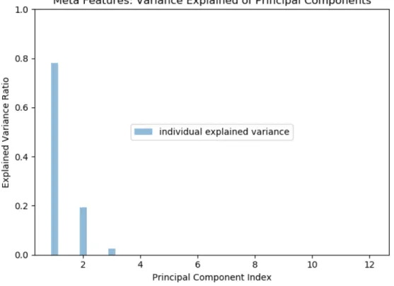
Due to potential redundant information being contained within the meta features and the number of features being greater than the number of datasets, the dimen-sionality of the meta features is reduced using PCA. Figure 4 graphs the variance explained by each principal component. Four principal components explain 100% of the variability in the meta features. However, three principal components are chosen for the dimension reduction to graph the meta features in 3-dimensional space. These three principal components explain 99.7% of the variability in the data. The loading vectors for these principal components are shown in Table 6.

(46)

T able 6. Principal Comp onen t Loading V ector Principal Comp onen t Loading V ector Ro ws Columns Ro ws-Cols Ratio Num b er Discrete Max n um factors Min n um factors Avg n um factors Num b er Con tin uous Gradien t Avg Gradien t Min Gradien t Max Gradien t Std 1 0.3257 0.3265 -0.0030 0.3265 0.3249 -0.0677 0.2807 0.2555 0.3266 -0.3266 0.3266 0.3263 2 0.0332 -0.0118 0.6458 -0.0076 0.0662 0.5997 0.3314 -0.3281 0.0026 -0.0071 0.0059 0.0069 3 0.1126 0.0555 0.2998 0.0650 0.0556 -0.6280 -0.1408 -0.6765 0.0459 -0.0503 0.0470 0.0915

(47)

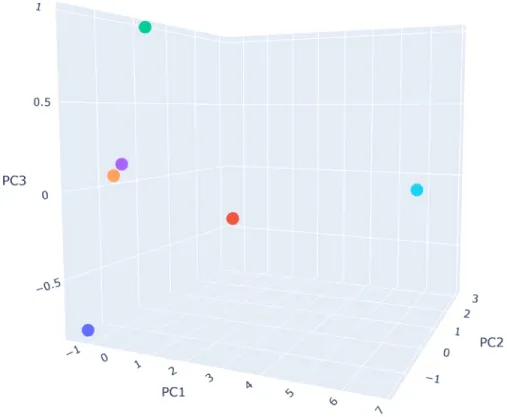
The projection of the meta features into the principal components space is shown in Figure 5. Additionally, Table 7 gives the coordinates for each dataset shown in Figure 5.

Figure 5. Meta Features Projected in Principal Component Space

Table 7. Meta Features in Principal Component Space

Dataset PC1 PC2 PC3

Heart -1.2211 -1.7051 -0.7891

Spam -1.3708 3.1317 -0.4216

Bank Personal Loan -1.4891 0.1232 0.9887

Framingham -1.3349 -0.7152 0.1298

Math Placement -1.4249 -0.8649 0.0637

Credit Card Fraud 6.8408 0.0303 0.0285

All datasets except Credit Card Fraud are nearly coplanar in the Principal Compo-nent 1 plane. The euclidean distance between the Framingham and Math Placement

(48)

datasets is 0.1868. Therefore, the algorithms are expected to perform similarly on these two datasets if the distribution of the response is similar between the two.

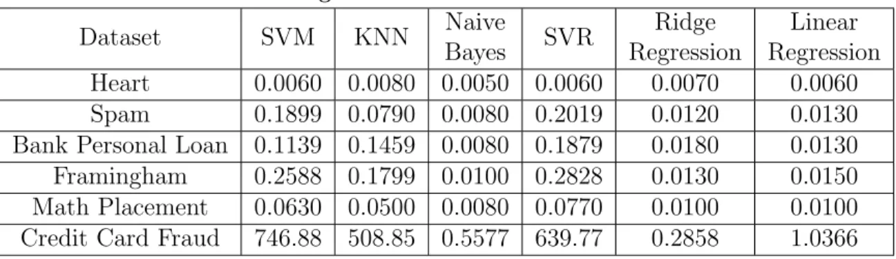
Table 8 gives the time to execute each a ∈ A for each p∈ P. Since KNN, SVM and SVR scale poorly with the size of the dataset, Credit Card fraud dataset has the worst time performance.

Table 8. Algorithm Execution Time in Seconds

Dataset SVM KNN Naive Bayes SVR Ridge Regression Linear Regression Heart 0.0060 0.0080 0.0050 0.0060 0.0070 0.0060 Spam 0.1899 0.0790 0.0080 0.2019 0.0120 0.0130

Framingham 0.2588 0.1799 0.0100 0.2828 0.0130 0.0150

Math Placement 0.0630 0.0500 0.0080 0.0770 0.0100 0.0100

NRMSE

In this section, the six datasets in the problem space P, have their algorithm performance predicted using the metric NMRSE. The true algorithm performance is ranked for each dataset using this metric and the algorithm ranking returned by the meta learner recommendation system are evaluated.

Table 9 shows each algorithms’ performance using the metric NRMSE. Note that this metric is not normally to evaluate classifiers. The rankings of each algorithm

a ∈ A is given in Table 10. Using NRMSE, SVR is the true best performing algo-rithm in 50% of the datasets, while its classification counterpart SVM is the worst performing algorithm in 33.33% of the datasets. Overall, SVR is always in the top third performing algorithms, while SVM is in the bottom two, in 66.7% of the datasets.

(49)

Table 9. Dataset Actual NRMSE

Dataset SVM KNN Naive Bayes SVR Ridge Regression Linear Regression

Heart 0.4149 0.4527 0.3841 0.4049 0.4049 0.4049

Spam 0.3787 0.3670 0.4950 0.3801 0.4736 0.4736

Framingham 0.5638 0.4076 0.4167 0.3904 0.3904 0.3904

Math Placement 0.5493 0.5364 0.5403 0.4930 0.5138 0.5138

Table 10. Dataset Actual NRMSE Ranking

Heart 5 6 1 3 3 3

Spam 2 1 6 3 4.5 4.5

Bank Personal Loan 2 3 6 1 4.5 4.5

Framingham 6 4 5 2 2 2

Math Placement 6 4 5 1 2.5 2.5

Credit Card Fraud 5 2 6 1 3 4

To predict the performance metric NRMSE, SVR is the meta learner with the meta features as the input and each algorithms’ NRMSE as the target variable. Leave one out validation gives the final predicted NRMSE of each dataset.

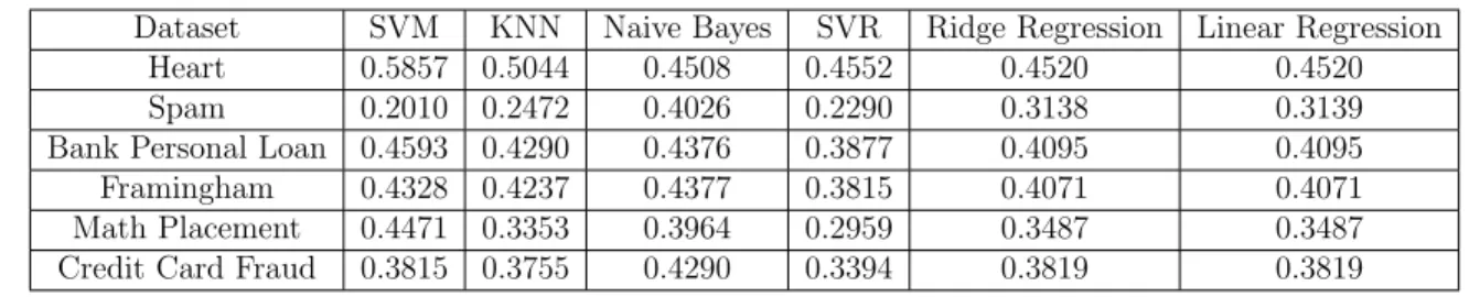
The final predicted NRMSE of the meta models is given in Table 11 and the predicted algorithm ranking is given in Table 12. The meta learner ranks SVR as the top performing algorithm for 66.7% of the datasets, which could be due to the true performance of that algorithm ranking in the top three for all datasets.

Table 11. Dataset Predicted NRMSE

Heart 0.5857 0.5044 0.4508 0.4552 0.4520 0.4520

Spam 0.2010 0.2472 0.4026 0.2290 0.3138 0.3139

Framingham 0.4328 0.4237 0.4377 0.3815 0.4071 0.4071

Math Placement 0.4471 0.3353 0.3964 0.2959 0.3487 0.3487

(50)

Table 12. Dataset Predicted NRMSE Rankings

Heart 6 5 1 4 2 3

Spam 1 3 6 2 4 5

Bank Personal Loan 6 4 5 1 2 3

Math Placement 6 2 5 1 3 4

Credit Card Fraud 3 2 6 1 4.5 4.5

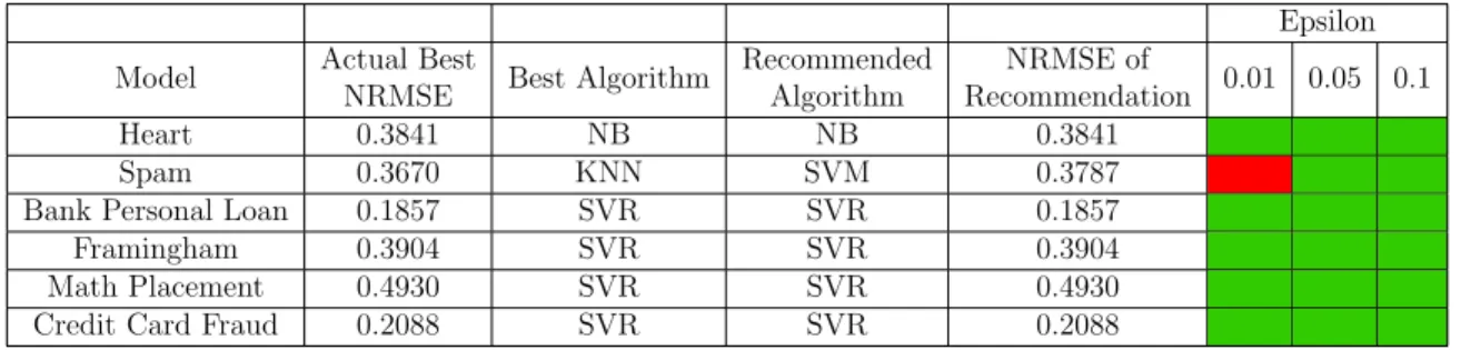
The evaluation of the meta learner using NRMSE as a performance metric for classification problems is given by Table 13. Using NRMSE as the performance metric with classification problems, causes the system to recommend the usage of the actual best performing algorithm in two out of the six datasets. A priori knowledge of each

a ∈ A performance for all p ∈ P, allows the NRMSE of the recommendation to be compared with the known best algorithm. In Table 13, relaxing the tolerance of a hit to be within 10% of the actual best NRMSE, improves the hit rate to 50%.

Table 13. NRMSE Recommendation Rating

Epsilon Model Actual Best

NRMSE Best Algorithm

Recommended Algorithm NRMSE of Recommendation 0.01 0.05 0.1 Heart 0.3841 NB NB 0.3841 Spam 0.3670 KNN SVM 0.3787 Bank Personal Loan 0.1857 SVR SVR 0.1857 Framingham 0.3904 SVR SVR 0.3904 Math Placement 0.4930 SVR SVR 0.4930 Credit Card Fraud 0.2088 SVR SVR 0.2088

(51)

NRMSE using Class Probabilities

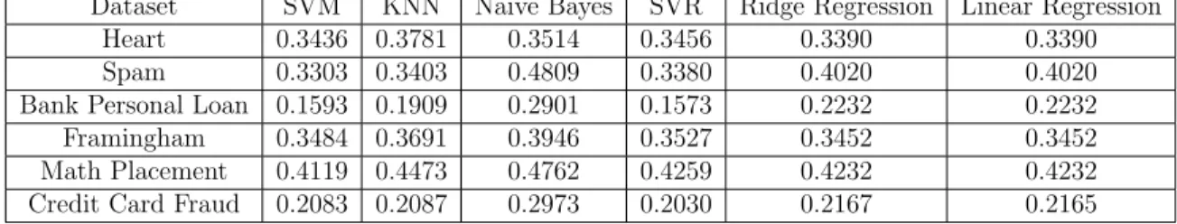
In this section, the six datasets in the problem space P, have their algorithm performance predicted using the metric NMRSE calculated using class probabilities. In this case, the predicted values ˆy∈[0,1]. The true algorithm performance is ranked for each dataset using this metric and the algorithm ranking returned by the meta learner recommendation system are evaluated.

Table??shows each algorithms performance using the metric different calculation of NRMSE. Like the previous section, note that this metric is not normally to evaluate classifiers. The rankings of each algorithm a∈A is given in Table ??.

Table 14. Dataset Actual NRMSE using Class Probabilities

Heart 0.3436 0.3781 0.3514 0.3456 0.3390 0.3390

Spam 0.3303 0.3403 0.4809 0.3380 0.4020 0.4020

Framingham 0.3484 0.3691 0.3946 0.3527 0.3452 0.3452

Math Placement 0.4119 0.4473 0.4762 0.4259 0.4232 0.4232

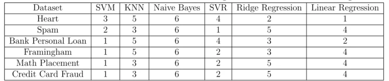
Table 15. Dataset Actual NRMSE using Class Probabilities Ranking

Heart 3 6 5 4 1 2

Spam 1 3 6 2 5 4

To predict the performance metric, NRMSE calculated using the class probabili-ties, SVR is the meta learner with the meta features as the input and each algorithms’ NRMSE as the target variable. Leave one out validation gives the final predicted NRMSE of each dataset.

The final predicted NRMSE using class probabilities of the meta models is given in Table ?? and the predicted algorithm ranking is given in Table ??. SVM ranks

(52)

in the top three for all datasets and Naive Bayes ranked last in 5_⁄₆ _{datasets. Due to}

SVM’s performance on the datasets, the recommendation system predicted it as top performing algorithm in 66.67% cases.

Table 16. Dataset Predicted NRMSE using Class Probabilities

Heart 0.3436 0.3794 0.3855 0.3674 0.3229 0.3229

Spam 0.2335 0.2625 0.3832 0.2236 0.3217 0.3216

Framingham 0.3063 0.3410 0.3855 0.3187 0.3232 0.3232

Math Placement 0.2538 0.2845 0.3855 0.2550 0.3094 0.3093

Table 17. Dataset Predicted NRMSE using Class Probabilities Ranking Dataset SVM KNN Naive Bayes SVR Ridge Regression Linear Regression

Heart 3 5 6 4 2 1

Spam 2 3 6 1 5 4

The evaluation of the meta learner using this different NRMSE as a performance metric for classification problems is given by Table??. Using NRMSE as the perfor-mance metric with classification problems causes the system to recommend the usage of the actual best performing algorithm in only one out of the six datasets. However, despite this low hit ratio, the actual NRMSE of the recommendation is within 5% of the true best. Thus, once the hit ratio is relaxed to the recommendation being 5% of the true best, then it is improved to 100%.

(53)

Table 18. NRMSE using Class Probabilities Recommendation Rating

NRMSE Best Algorithm

Recommended Algorithm NRMSE of Recommendation 0.01 0.05 0.1 Heart 0.3390 RR LR 0.3390 Spam 0.3303 SVM SVR 0.3380 Bank Personal Loan 0.1573 SVR SVR 0.1593 Framingham 0.3452 RR SVM 0.3484 Math Placement 0.4119 SVM SVM 0.4119 Credit Card Fraud 0.2030 SVR SVM 0.2083

F1 Score

In this section, the six datasets in the problem space P, have their algorithm performance predicted using the metric F1 score. F1 score is a single metric that is useful if one value is desired to compare two classifiers. It is the harmonic mean of precision and recall.

Since the algorithms support vector regression, linear regression and ridge regres-sion are not normally used for classification, a threshold is set to assign class labels. Figure 14 shows that a decision threshold of 0.5 is not optimal for the Credit Card Dataset using SVR. Additional, graphs of the F1 score versus the decision threshold for the other dataset algorithm combinations are included in Appendix A.

(54)

Figure 6. SVR Credit Card Fraud F1 vs Threshold

Table 19 shows each algorithms performance using the metric F1 score. The rankings of each algorithm a ∈A is given in Table 20. SVM and KNN are typically the top performing algorithms except for the Heart dataset.

Table 19. Dataset Actual F1 Score

Heart 0.8346 0.8175 0.8636 0.8485 0.8551 0.8551

Spam 0.8101 0.8166 0.5933 0.7966 0.6158 0.6158

Framingham 0.3708 0.1413 0.2743 0.0823 0.0089 0.0089

Math Placement 0.7494 0.7972 0.7649 0.8362 0.8219 0.8219

(55)

Table 20. Actual F1 Score Rankings

Heart 5 6 1 4 2.5 2.5

Spam 2 1 6 3 4.5 4.5

Framingham 1 3 2 4 5.5 5.5

Like the previous performance metrics, to predict F1 score, SVR with a radial ba-sis function kernel is the meta learner with the meta features projected to 3-dimension space as the input and each algorithms’ F1 score as the target variable. Additionally, the default parameters of python’s implementation of SVR are used and the hyper-parameter gamma is set to scale which is given by Equation (46) and the penalty hyperparameter C is set to one. Leave one out validation gives the final predicted F1 score of each dataset. The final predicted F1 score of the meta models is given in Table 21 and algorithm ranking is given in Table 22. Similar to the usage of NRMSE as performance metric, the recommendation gives SVR as the best or second best performing algorithm for all six datasets because its true performance is in the top three in 66.67% of the datasets used to construct the meta learner.

Table 21. Dataset Predicted F1 Score

Heart 0.6143 0.7181 0.5824 0.7520 0.5609 0.5607

Spam 0.7716 0.6392 0.5403 0.6741 0.5699 0.5698

Framingham 0.7324 0.7191 0.7084 0.7487 0.7119 0.7119

Math Placement 0.6952 0.6257 0.5857 0.6877 0.5704 0.5704

(56)

Table 22. Predicted F1 Score Rankings

Heart 3 2 4 1 5 6

Spam 1 3 6 2 4 5

The evaluation of the meta learning recommendation system using F1 score as a performance metric is given by Table 23. Using F1 score as the performance met-ric with classification problems results in a worse hit ratio than using NRMSE. The recommendation system correctly selects the true best performing algorithm in one case. If the criteria for a hit is relaxed to the system’s recommendation being within 5% of the actual best algorithm, then the hit ratio improves to 66.67%. Addition-ally, relaxing the tolerance of a hit to being within 5% of the actual best algorithm, improves the hit rate to 66.67%.

Table 23. F1 Score Recommendation Rating

Precision Best Algorithm

Recommended Algorithm Precision of Recommendation 0.01 0.05 0.1 Heart 0.8636 NB SVR 0.8485 Spam 0.8166 KNN SVM 0.8101 Bank Personal Loan 0.8159 SVM SVR 0.7890 Framingham 0.3708 SVM SVR 0.0823 Math Placement 0.8362 SVR SVM 0.7494 Credit Card Fraud 0.6490 SVR SVR 0.6490

(57)

Precision

In this section, the six datasets in the problem space P, have their algorithm performance predicted using the metric precision. As stated in the literature review, precision is the accuracy of positive predictions and there is a trade off of this metric and recall.

Since the algorithms SVR, LR and RR are not normally used for classification, a threshold is necessary to assign class labels. Figure 7 shows that a decision threshold of 0.5 is not optimal for the Credit Card Dataset using SVR. Additional, graphs of the precision and recall versus the decision threshold for the other dataset algorithm combinations are included in Appendix A.

(58)

Table 24 shows each algorithms performance using the performance metric pre-cision. The rankings of each algorithm a ∈ A is given in Table 25. The regression algorithms used classification true precision ranks in the top three of the algorithms used for 66.67% of the datasets.

Table 24. Dataset Actual Precision

Heart 0.8689 0.7887 0.8636 0.8485 0.8194 0.8194

Spam 0.8466 0.8804 0.8568 0.8937 0.9457 0.9457

Framingham 0.2655 0.3333 0.3780 0.5000 0.5000 0.5000

Math Placement 0.8568 0.7627 0.8416 0.7695 0.7569 0.7569

Table 25. Dataset Actual Precision Rankings

Heart 1 6 2 3 4.5 4.5

Spam 6 4 5 3 1.5 1.5

Like the previous performance metrics, to predict precision, SVR with a radial ba-sis function kernel is the meta learner with the meta features projected to 3-dimension space as the input and each algorithms’ precision as the target variable. Leave one out validation gives the predicted precision of the dataset.

The final predicted precision of the meta models is given in Table 26 and algorithm ranking is given in Table 27.

Table 26. Dataset Predicted Precision

Heart 0.7359 0.5616 0.6238 0.5676 0.5368 0.5359

Spam 0.6480 0.9286 0.5260 0.9406 0.9621 0.9621

Framingham 0.7659 0.8507 0.7256 0.8625 0.8585 0.8585

Math Placement 0.6759 0.7244 0.5783 0.7641 0.7563 0.7563

(59)

Table 27. Dataset Predicted Precision Ranking

Heart 1 4 2 3 5 6

Spam 5 4 6 3 1.5 1.5

Framingham 5 4 6 1 2.5 2.5

The evaluation of the meta learning recommendation system using precision as a performance metric is given in Table 28. Using precision as the performance metric with classification problems causes the system to recommend the usage of the actual best performing algorithm in half of the datasets used for this thesis. Relaxing the criteria for a hit does not improve the hit ratio.

Table 28. Precision Recommendation Rating

Precision Best Algorithm

Recommended Algorithm Precision of Recommendation 0.01 0.05 0.1 Heart 0.8689 SVM SVM 0.8689 Spam 0.9457 RR RR 0.9457

Bank Personal Loan 0.9718 RR SVM 0.7384 Framingham 0.5000 SVR SVR 0.5000 Math Placement 0.8568 SVM SVR 0.7695 Credit Card Fraud 0.9301 SVR RR 0.9301

(60)

Recall

In this section, the six datasets in the problem space P, have their algorithm performance predicted using the metric recall. Recall is the ratio of positive instances that are correctly detected by the classifier. It is also called true positive rate or sensitivity. A classifier with high recall but low precision will have many predicted labels that are incorrect when compared to the training labels. This classifier predicts many positives instances. On the other hand, a classifier with high precision but low recall will have many correct predictions when compared to the training labels but the classifier is predicting many negative instances [24]. Note, there is a precision recall trade off. Increasing recall will reduce precision and vice versa [17].

Table 29 shows each algorithms performance using the metric recall. Since recall is the accuracy of the positive predictions, it will low for algorithms that do not predict many positive instances. This is why the recall for the Framingham and Credit Card data sets are much lower for the algorithms SVR, LR and RR. The rankings of each algorithm a ∈A is given in Table 30. SVM is the true best performing algorithm in 66.67% of the datasets.

Table 29. Dataset Actual Recall

Heart 0.8030 0.8485 0.8636 0.8485 0.8939 0.8939

Spam 0.7766 0.7614 0.4538 0.7186 0.4566 0.4566

Framingham 0.6143 0.0897 0.2152 0.0448 0.0045 0.0045

Math Placement 0.6660 0.8351 0.7010 0.9155 0.8990 0.8990

(61)

Table 30. Dataset Actual Recall Rankings

Heart 6 4.5 3 4.5 1.5 1.5

Spam 1 2 6 3 4.5 4.5

Framingham 1 3 2 4 5.5 5.5

Like the previous performance metrics, to predict recall, SVR with a radial basis function kernel is the meta learner with the meta features projected to 3 - dimensional space as the input and each algorithms’ recall as the target variable. Like the previous sections, the hyperparameters are set to the defaults. The predicted recall of the dataset that is left out during leave one out validation is the predicted precision of the meta modeler.

The final predicted recall of the meta models is given in Table 31 and algorithm ranking is given in Table 32.

Table 31. Dataset Predicted Recall

Heart 0.6417 0.6699 0.5991 0.6494 0.4059 0.4061

Spam 0.8879 0.6133 0.5802 0.6246 0.3693 0.3693

Framingham 0.7708 0.7273 0.7279 0.8113 0.6710 0.6710

Math Placement 0.7208 0.5743 0.6343 0.6368 0.4285 0.4285

Table 32. Dataset Predicted Recall Rankings

Heart 3 1 4 2 6 5

Spam 1 3 4 2 6 5

(62)

Table 33 shows evaluation of the meta learning recommendation system using recall as the performance metric. The meta learning recommendation system recom-mends the actual best performing algorithm 50% of the time. Additionally, relaxing the tolerance of a hit to being within 10% of the actual best algorithm, improves the hit rate to 66.67%.

Table 33. Recall Recommendation Rating

Recall Best Algorithm

Recommended Algorithm Recall of Recommendation 0.01 0.05 0.1 Heart 0.8939 RR KNN 0.8485 Spam 0.7766 SVM SVM 0.7766 Bank Personal Loan 0.9115 SVM SVM 0.9115 Framingham 0.6143 SVM SVR 0.0448 Math Placement 0.9155 SVR SVM 0.6660 Credit Card Fraud 0.6945 SVM SVM 0.6945

Figure 8 shows recalls versus the time to execute each algorithm for the Credit Card dataset. Since the dataset is large SVR, SVM and KNN had a slow execution time. The algorithm Naive Bayes Classifier dominates RR, LR, KNN and SVR. Naive Bayes does not dominate SVM but there is a practical difference in execution time. SVM had that best recall of 0.6945 but it took 12.45 minutes to execute that algorithm versus Naive Bayes which has a recall of 0.5423 but execute instantaneously on this dataset.

(63)

Figure 8. Credit Card Fraud Recall vs Time

Comparison

Table 34 and Table 35 show the actual and predicted algorithm ranking for each

dataset when the regression algorithms are removed. The hit rates improves to

66.67%.

Table 34. Recall Classification Algorithms Actual Ranking

Dataset SVM KNN Naive Bayes

Heart 3 2 1

Spam 1 2 3

Bank Personal Loan 1 3 2

Framingham 1 3 2

Math Placement 3 1 2

(64)

Table 35. Recall Classification Algorithms Predicted Ranking

Dataset SVM KNN Naive Bayes

Heart 2 1 3

Spam 1 2 3

Bank Personal Loan 1 2 3

Framingham 1 3 2

Math Placement 1 3 2

Credit Card Fraud 1 2 3

Table 36. Credit Card Fraud Evaluation Metrics Comparison

NRMSE

NRMSE Probabilitiesbilities

Precision

Recall

F1 Score

SVR

SVM

RR

SVM

SVR

Table 36 shows the comparison of the recommendation r0 of the Credit Card

Fraud dataset for each the member of the performance space z. For this dataset, the recommendation system gives the true best algorithm when NRMSE, Recall and F1 Score are the performance metric used to rank the algorithms. When using NRMSE as the evaluation metric, SVR is the recommended algorithm. This recommendation is correct. However, inspecting the confusion matrix for SVR shown in Table 72 shows that the algorithm is only classifying 49.84% of the fraudulent credit card transactions correctly. The performance metric recall changes the recommendation r0 to SVM. In this case, the confusion matrix shown in Table 37, reveals the amount of fraudulent transactions correctly classified improves to 69.45%. Additional, confusion matrices for every dataset, algorithm combination are in Appendix B.