clustering, visualization, and outlier detection
ACM Transactions on Knowledge Discovery from Data,New York : ACM,v. 10, n. 1, p. 5:1-5:51, Jul.
2015
http://www.producao.usp.br/handle/BDPI/51005
5
and Outlier Detection
RICARDO J. G. B. CAMPELLO, Department of Computer Sciences, University of S ˜ao Paulo, Brazil
DAVOUD MOULAVI, Department of Computing Science, University of Alberta, Canada
ARTHUR ZIMEK, Ludwig-Maximilians-Universit ¨at M ¨unchen, Germany
J ¨ORG SANDER, Department of Computing Science, University of Alberta, Canada
An integrated framework for density-based cluster analysis, outlier detection, and data visualization is introduced in this article. The main module consists of an algorithm to compute hierarchical estimates of the level sets of a density, following Hartigan’s classic model of density-contour clusters and trees. Such an algorithm generalizes and improves existing density-based clustering techniques with respect to different aspects. It provides as a result a complete clustering hierarchy composed of all possible density-based clusters following the nonparametric model adopted, for an infinite range of density thresholds. The resulting hierarchy can be easily processed so as to provide multiple ways for data visualization and exploration. It can also be further postprocessed so that: (i) a normalized score of “outlierness” can be assigned to each data object, which unifies both the global and local perspectives of outliers into a single definition; and (ii) a “flat” (i.e., nonhierarchical) clustering solution composed of clusters extracted from local cuts through the cluster tree (possibly corresponding to different density thresholds) can be obtained, either in an unsupervised or in a semisupervised way. In the unsupervised scenario, the algorithm corresponding to this postprocessing module provides a global, optimal solution to the formal problem of maximizing the overall stability of the extracted clusters. If partially labeled objects or instance-level constraints are provided by the user, the algorithm can solve the problem by considering both constraints violations/satisfactions and cluster stability criteria. An asymptotic complexity analysis, both in terms of running time and memory space, is described. Experiments are reported that involve a variety of synthetic and real datasets, including comparisons with state-of-the-art, density-based clustering and (global and local) outlier detection methods.
Categories and Subject Descriptors: H.2.8 [Database Mamagement]: Database Applications—Data mining; H.3.3 [Information Storage and Retrieval]: Information Search and Retrieval—Clustering; I.5.3 [Pattern Recognition]: Clustering—Algorithms
General Terms: Data Mining, Clustering, Algorithms
Additional Key Words and Phrases: Density-based clustering, hierarchical and nonhierarchical clustering, unsupervised and semisupervised clustering, data visualization, outlier detection, global/local outliers ACM Reference Format:
Ricardo J. G. B. Campello, Davoud Moulavi, Arthur Zimek, and J¨org Sander. 2015. Hierarchical density estimates for data clustering, visualization, and outlier detection. ACM Trans. Knowl. Discov. Data 10, 1, Article 5 (July 2015), 51 pages.
DOI: http://dx.doi.org/10.1145/2733381
This work was partially supported by NSERC (Canada), FAPESP (Brazil, grant #2013/18698-4 and grant #2010/20032-6), and CNPq (Brazil, grant #304137/2013-8 and grant #201239/2012-4).
Authors’ addresses: R. J. G. B. Campello; email: campello@icmc.usp.br; D. Moulavi; email: moulavi@ualberta.ca; A. Zimek; email: zimek@dbs.ifi.lmu.de; J. Sander; email: jsander@ualberta.ca. For part of this project, Ricardo J. G. B. Campello worked in the Department of Computing Science at the University of Alberta, Canada, on a sabbatical leave from the University of S ˜ao Paulo at S ˜ao Carlos, Brazil. Permission to make digital or hard copies of part or all of this work for personal or classroom use is granted without fee provided that copies are not made or distributed for profit or commercial advantage and that copies show this notice on the first page or initial screen of a display along with the full citation. Copyrights for components of this work owned by others than ACM must be honored. Abstracting with credit is permitted. To copy otherwise, to republish, to post on servers, to redistribute to lists, or to use any component of this work in other works requires prior specific permission and/or a fee. Permissions may be requested from Publications Dept., ACM, Inc., 2 Penn Plaza, Suite 701, New York, NY 10121-0701 USA, fax+1 (212) 869-0481, or permissions@acm.org.
c
2015 ACM 1556-4681/2015/07-ART5 $15.00 DOI: http://dx.doi.org/10.1145/2733381
mining the estimate...” [Silverman 1986]. 1.1. Multi-Level Mode Analysis for Clustering
In cluster analysis, there is also a contrast between parametric and nonparametric approaches. For example, from a statistical point of view, popular algorithms such ask -means and EMGM (Expectation Maximization for Gaussian Mixtures) correspond to a
parametricapproach in which an unknown PDF is assumed to be composed of a mixture ofkGaussian distributions, each of which is associated to one of thekclusters supposed to exist in the data (wherektypically must be provided by the analyst) [Bishop 2006]. As a result, these algorithms produce a predetermined number of clusters that tend to be of convex (hyper-spherical or hyper-elliptical) shape. Notice that the limitation to convex-shaped clusters is also present in other traditional clustering algorithms, such as average linkage, Ward’s, and related techniques [Jain and Dubes 1988], which do not make explicit use of parametric models. In common among these methods there is an underlying principle of “minimum variance”, in the sense that all of them directly or indirectly seek to minimize a given measure of variance within clusters. The limi-tations of such methods, including their inability to find clusters of arbitrary shapes, have encouraged the development of alternative clustering paradigms and related al-gorithms that allow for more complex structures to be found in data [Xu and Wunsch II 2005, 2009]. Among those, density-based clustering [Tan et al. 2006; Ester 2009; Sander 2010; Kriegel et al. 2011] stands as a popular paradigm in which algorithms explicitly or implicitly incorporate elements from the theory ofnonparametricdensity estimation [Hwang et al. 1994].
The first attempt at practical data clustering based on nonparametric density esti-mates seems to be theOne Level Mode Analysis method and its hierarchical version (Hierarchical Mode Analysis—HMA) published by Wishart [1969] in the late 1960s. In that seminal article, Wishart listed thirteen clustering algorithms based on the “min-imum variance” principle, which had already become widespread at that time, and elaborated on a number of objections to those algorithms, discussing why they may fail when applied to real world problems. He also elaborated on the limitations of the single-linkage model [Sneath 1957; Johnson 1967] and proposed a novel approach to the clustering problem, thereby establishing the grounds for what is nowadays known as
density-based clustering. Indeed, the methods proposed by Wishart [1969] anticipated a number of conceptual and practical key ideas that have also been used by modern density-based clustering algorithms. Conceptually, for example, when referring to an estimate f of a given (possibly multivariate) PDF and a density thresholdλ, Wishart observed that “...if f has two or more modes at the level of probability λ, then the covering will be partitioned into two or more disjoint connected subsets of points”. This
idea was formalized and extended later by Hartigan [1975], who defined the concepts ofdensity-contour clustersanddensity-contour tree. These concepts play an important role as a formal probabilistic model for density-based clustering and, indeed, they have been explicitly or implicitly used as such by many algorithms belonging to this class.
For the sake of simplicity and without any loss of generality, let us consider that the observations (data objects) are described by a single continuous-valued variable (attribute),x, and that a bounded, continuous density function f(x) is defined for each
xas a value proportional to the number of points per unit volume atx. Then, according to Hartigan’s model [Hartigan 1975], adensity-contour clusterof f(x) at a given density levelλis a subsetC⊂ such that: (i) everyx∈Csatisfies f(x)≥λ; (ii)Cis connected; and (iii)Cis maximal. The density-contour clusters at a given level λ are therefore the collection of maximal connected subsets of thelevel set defined as {x| f(x) ≥ λ}. Thedensity-contour treeis the tree of nested clusters that is conceptually conceived by varying the thresholdλ. Notice that these concepts can be readily extended to more general domains other than continuous-valued densities in the real coordinates space. The power of Hartigan’s model is mainly due to the following reasons: (i) it allows the concept ofnoise to be modeled as those objects lying in nondense regions of the data space, that is, objects for which the density is below a certain threshold. This is of particular importance in cluster analysis as it breaks down the common yet usually unrealistic assumption that observations must belong to clusters and therefore they must all be clustered indistinctly; (ii) it allows clusters of varied shapes to be modeled as the connected components of the density level sets. Such components are not restricted to the domain of a single mode (peak) of the density function, they can possibly represent the union of multiple modes (depending on the density threshold); and (iii) it allows one to model the presence of nested clusters of varied densities in data, through the hierarchical relationships described by the density-contour tree.
For the reasons mentioned earlier, most density-based clustering algorithms are, in essence, strictly or loosely based on Hartigan’s model.1The differences basically rely
on the way the density fand the components of a level set are estimated. For Wishart’s one level mode analysis method (with parametersrandκ), for example, it can be shown that the results correspond to the use of an estimator of connected components given by the union of balls of radiusr/2, a K nearest neighbor (K-NN) density estimate f
with K =κ, and a density thresholdλas a function of r(or, equivalently, f can also be seen as a kernel-based density equipped with square-wave kernels of widthrand
λas a function ofκ). The same holds true for the popular algorithm DBSCAN [Ester et al. 1996] if one denotes its parameters, neighborhood radius and minimum number of objects within the neighborhood, as r and κ, respectively. DBSCAN is, however, computationally more sophisticated and scalable as it makes use of efficient indexing structures. There is also a conceptual difference since, in DBSCAN, those non-dense objects that lie in the neighborhood of dense objects, the so-calledborder objects, are assigned to clusters even though their density is below the established threshold. Notice that such a strategy makes DBSCAN only loosely in conformity with Hartigan’s model.2This is also the case for the well-known algorithm DENCLUE [Hinneburg and
Keim 1998, 2003; Hinneburg and Gabriel 2007], which uses a general kernel-based density estimate as well as a gradient-based approach to decide which objects should
1In contrast, works such as [Fukunaga and Hostetler 1975; Coomans and Massart 1981] make the oversim-plistic assumption that each mode of the density f corresponds to a cluster and, then, they simply seek to assign every data object to one of these modes (according to some hill-climbing-like heuristic).
2Wishart’s one level mode analysis method also does not follow strictly Hartigan’s model if the optional postprocessing stage of that method is performed, in which the non-dense objects are arbitrarily assigned to the “nearest” cluster.
as those in Wishart [1969], Wong and Lane [1983], Ankerst et al. [1999], Sander et al. [2003], Brecheisen et al. [2004], Chehreghani et al. [2008], Stuetzle and Nugent [2010], Sun et al. [2010], Gupta et al. [2010], and Campello et al. [2013a], which are able to provide more elaborated descriptions of a dataset at different degrees of granularity and resolution.
Hierarchical models are indeed able to provide richer descriptions of clustering struc-tures than those provided by flat models. In spite of this, applications in which the user also needs a flat solution are common, either for further manual analysis by a domain expert or in automated KDD processes in which the output of a clustering algorithm is the input of a subsequent data mining procedure—for example, pattern recognition based on image segmentation. In this context, the extraction of a flat clustering from a hierarchy may be advantageous when compared to the extraction directly from data by a partitioning-like (i.e., nonhierarchical) algorithm. The reason is that hierarchical models describe data from multiple levels of specificity/generality, providing a means for exploration of multiple possible solutions from different perspectives while having a global picture of the cluster structure available.
1.2. Global and Local Outlier Detection
Similar as for clustering, parametric, statistical approaches for unsupervised outlier detection (identification, rejection) fit certain distributions to the data by estimating the parameters of these distributions from the given data [Grubbs 1950; Barnett 1978; Beckman and Cook 1983; Hodge and Austin 2004; Agyemang et al. 2006; Hadi et al. 2009]. For example, when assuming a Gaussian distribution, a commonly used rule of thumb, known as the “3·σ-rule”, is that points deviating more than three times the standard deviation from the mean of a normal distribution may be considered outliers [Knorr and Ng 1997b]. Classical textbooks [Hawkins 1980; Barnett and Lewis 1994] discuss numerous tests for different distributions. The tests are optimized for each distribution dependent on the specific parameters of the corresponding distribution, the number of expected outliers, and the space where to expect an outlier.
A problem with parametric approaches is that distribution parameters such as mean, standard deviation, and covariances are rather sensitive to the presence of outliers. Possible effects of outliers on the parameter estimation have been termed“masking”
and“swamping”. Outliers canmask their own presence by influencing the values of the distribution parameters (resulting in false negatives), orswampinliers to appear as outlying due to the influenced parameters (resulting in false positives) [Pearson and Chandra Sekar 1936; Beckman and Cook 1983; Barnett and Lewis 1994; Hadi et al. 2009]. Furthermore, these approaches are deemed to assume a specific type of distribution.
Nonparametric approaches for outlier detection do not assume a specific distribu-tion of the data, but estimate (explicitly or implicitly) certain aspects of the probability density. Nonparametric methods include, for instance, the well-known “distance-based” methods [Knorr and Ng 1997b; Ramaswamy et al. 2000; Angiulli and Pizzuti 2002] and also “density-based” methods such as LOF (local outlier factor) [Breunig et al. 2000] and its many variants. An important categorization of these approaches distinguishes “local” versus “global” approaches. Although this categorization is not strictly dichoto-mous but there are degrees of locality [Schubert et al. 2014b], these categories reflect the nature of outliers that can be found by local or by global methods. Global outliers are outliers that are unusual w.r.t. the complete database. Local outliers are outliers that are unusual w.r.t. a local selection of the database only, such as anε-range query or theK-NNs, but that would not necessarily look suspicious when compared globally to the complete database. Not only are there degrees of locality in the design of methods, but also a local method such as LOF could be used (or rather abused) in a global way by considering the complete database as the NNs (i.e.,K=database size). This would be not in the spirit of the method but even so, one method with one parametrization is either local (with a certain degree) or global, but not both at the same time. It would be rather the spirit of LOF to choose the size of the neighborhood in a way to at least include some objects of the nearest cluster for an outlier while not including objects of another cluster for inliers. Choosing the right Kfor the neighborhood, of course, is a task unsolvable without knowing the data already. Thus, when choosing a method and a parametrization (such as neighborhood size), the users have to decide which kind of outliers, local or global, they are interested in.
The problem of having to select a particular threshold that inherently limits the types of outliers that a local method can detect in a given dataset (which may contain both global and local outliers) has also been recognized by Papadimitriou et al. [2003], who proposed the method LOCI that tries to address this problem. LOCI is probably the first, and so far only, attempt at finding for each point a neighborhood that is specific to the point in determining whether the point is an outlier or not. Depending on the distance that defines the neighborhood, a point can be a local outlier in some sense or even a global outlier. However, LOCI considers circular neighborhoods (just like LOF and related methods, yet at different distances around a point), which may not take the relevant structure of the data properly into account. Circular neighborhoods, at large scales, will typically contain “neighbors” from multiple, distant clusters whose properties can be considered as unrelated to the point at the center of the sphere, yet they are taken into account in the calculation of its outlier score.
In this article, we argue that by basing an outlier model on hierarchical density estimates, one can adapt not only to locally different density-levels (such as LOF and its variants) but also to locally different notions of “local”. Traditionally, each query object’s outlierness is assessed w.r.t. some reference set (such as alocal, circular neighborhood or the global database). In our approach, for each query object, the scope of a reference set of objects is chosen dynamically and based on the closest structurewithin the density-based hierarchy. By doing so, the locally suitable choice could actually be global for some objects while being strictly local for other objects. In any case, the most meaningful reference structure for a point is the “nearest” cluster in the hierarchical cluster hierarchy, as opposed to all points in some sphere around the point. This avoids comparing outliers to other outliers or unrelated clusters, as it could happen for a local method or LOCI; it also enables the user to find both global and local outliers and be able to relate them to the overall clustering structure within one efficient approach. Compared to previous methods, our approach represents somewhat of a paradigm shift in what constitutes meaningful neighborhoods for the determination of outlier scores. However, we argue that the outlier model we propose
we introduce in this article depend on the hierarchy of density estimates and its shape as a whole, rather than on a single “snapshot” taken at a particular, arbitrary level. We advocate that the problems of clustering and outlier detection should be treated simultaneously rather than separately (provided that this can be done properly) for two reasons: (i) when referring to an outlier asan observation that deviates so much from other observations as to arouse suspicions that it was generated by a different mechanism, as in the classical definition by Hawkins [1980], one is obviously assuming the existence of one or more mechanisms responsible for generating the observations deemed nonsuspicious. The modeling of such mechanisms seems to be, therefore, an important (if not fundamental) step towards the detection of suspicious observations as outliers. Intuitively, clusters are natural candidates for this task; and (ii) an out-lier is not always viewed as an observation that deviates too much fromallthe other observations. In fact, in some application domains outliers may actually refer to obser-vations that are similar to each other for they are generated by the same mechanism, although they are typically less frequent than and deviate from other observations (e.g., certain types of frauds or genetic mutations following a common pattern). These outliers can still be modeled and detected as clusters which are typically smaller in size or volume and possibly farther apart from other clusters.
1.3. Contributions
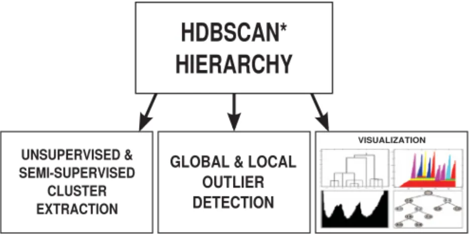
In this article, we introduce a complete framework for density-based clustering, outlier detection, and visualization. The core of the framework is a method based on nonpara-metric density estimates that gives rise to a hierarchical clustering algorithm HDB-SCAN* (Hierarchical DBSCAN*). HDBSCAN* follows Hartigan’s model of density-contour clusters/trees and improves existing density-based clustering algorithms w.r.t. different aspects (to be further elaborated in the related work section). It provides as a result a complete clustering hierarchy composed of all possible density-based clusters following the nonparametric model adopted, for an infinite range of density thresholds, and from which a simplified cluster tree can be easily extracted by using Hartigan’s concept ofrigid clusters[Hartigan 1975].
The proposed framework is illustrated in Figure 1. The hierarchy and the cluster tree produced by the central module (HDBSCAN*) can be postprocessed for multiple tasks. For instance, they are particularly suitable for interactive data exploration, as they can be easily transformed and visualized in different ways, such as an OPTICS reachability plot [Ankerst et al. 1999; Sander et al. 2003], a silhouette-like plot [Gupta et al. 2010], a detailed dendrogram, or a compacted cluster tree. In addition, for ap-plications that expect a nonhierarchical partition of the data, the clustering hierarchy can also be postprocessed so that a flat solution—as the best possible nonhierarchical
Fig. 1. Proposed framework for hierarchical & nonhierarchical density-based clustering, global/local outlier detection, and data visualization.
representation of the data in some sense—can be extracted. The traditional approach to get a flat solution from a hierarchical clustering is to perform a global horizontal cut through one of the levels of the hierarchy, but this approach inherits all the limi-tations we discussed earlier regarding the use of a single density threshold. For this reason, we instead advocate the use of a method by which a flat solution composed of clusters extracted from local cuts through the cluster tree (possibly corresponding to different density thresholds) can be obtained, either in an unsupervised or even in a semisupervised way. For the unsupervised scenario, we describe an algorithm that provides a globally optimal solution to the formal problem of maximizing the overall stability of the extracted clusters, for which a cluster stability measure is formulated. If partially labeled objects or instance-level constraints of the typeshould-link and
should-not-linkare provided by the user (semisupervised scenario), the algorithm can solve the problem by considering both constraint violations/satisfactions and cluster stability criteria. Finally, besides the clustering and visualization tasks, the density-based hierarchy produced by HDBSCAN* can also be used as the basis for a novel, effective, and efficient outlier detection method, as illustrated in Figure 1. The method we propose for the outlier detection module unifies both the global and local flavors of the outlier detection problem into a single definition of an outlier detection measure, called GLOSH (Global-Local Outlier Scores from Hierarchies), which also attempts at reconciling those more statistically inclined and those more database oriented methods for unsupervised outlier detection, by means of a nonparametric approach.
In detail, we make the following contributions within our proposed framework: (1) For the core module of the framework, we present and discuss in details
HDB-SCAN* as a hierarchical clustering method that generates a complete density-based clustering hierarchy from which a simplified cluster tree composed only of the most significant clusters can be easily extracted.
(2) We describe and discuss different ways of visualizing the HDBSCAN* results. (3) We present a measure of cluster stability for the purpose of extracting a flat
clus-tering solution from local cuts (possibly corresponding to different density levels) through the HDBSCAN* hierarchy; we formulate the task of extracting such a flat solution as an optimization problem in which the overall stability of the composing clusters (unsupervised scenario) and/or the fraction of instance-level constraints that are satisfied (semisupervised scenario) are maximized; and we describe an algorithm that finds the globally optimal solution to this problem.
(4) We propose GLOSH as a new, effective, and efficient outlier detection measure, which is possibly unique in that it can simultaneously detect both global and local
to be specialized and instantiated for use with each different type of hierarchy. The current article introduces and experimentally evaluates a new specialization for the HDBSCAN* hierarchy. Finally, the work described here on outlier detection presents completely new ideas and original material that has not been introduced elsewhere. 1.4. Outline of the Article
The remainder of this article is organized as follows. In Section 2, we redefine DBSCAN in a way that makes it more consistent with Hartigan’s model. Then, in Section 3, we present and provide an extensive description and discussion of the algorithm HDB-SCAN*. In Section 4, we discuss some different alternatives for the visualization of the HDBSCAN* results. In Section 5, we pose the problem of extracting a nonoverlapping collection of clusters from the HDBSCAN* hierarchy as an optimization problem, and describe an algorithm to solve this problem in an unsupervised or semisupervised way. In Section 6, we propose GLOSH, a novel outlier detection method, and describe a simple procedure to compute the corresponding outlier scores from the HDBSCAN* hierarchy. We discuss related work in Section 7. In Section 8, we present an extensive experimental evaluation involving real and synthetic data as well as comparisons with state-of-the-art algorithms for density-based clustering and for global and local outlier detection. Section 9 concludes the article.
2. DBSCAN REVISITED—THE ALGORITHM DBSCAN*
LetX= {x1, . . . ,xn}be a dataset containingndata objects, each of which is described by an attribute vector,x(·). In addition, letDbe (conceptuallyonly) ann×nsymmetric
matrix containing the distances d(xp,xq) between pairs of objects of X in a metric space3. In the following, we define the density-based clustering algorithm DBSCAN*
as in our preliminary work [Campello et al. 2013a], which differs from DBSCAN [Ester et al. 1996] in that the clusters are defined based oncore objectsalone.
Definition2.1 (Core and Noise Objects). An objectxpis called acore objectw.r.t.εand
mptsif itsε-neighborhood contains at leastmptsmany objects, that is, if|Nε(xp)| ≥mpts,
where Nε(xp) = {x ∈ X|d(x,xp) ≤ ε}and | · |denotes cardinality. An object is called
noiseif it is not a core object.
Definition2.2 (ε-Reachable). Twocoreobjectsxpandxqareε-reachablew.r.t.εand
mptsifxp∈Nε(xq) andxq∈Nε(xp).
Definition2.3 (Density-Connected). Twocoreobjectsxpandxqaredensity-connected w.r.t.εandmptsif they are directly or transitivelyε-reachable.
Definition2.4 (Cluster). AclusterCw.r.t.εandmptsis a non-empty maximal subset ofXsuch that every pair of objects inCis density-connected.
Based on these definitions, we can devise an algorithm DBSCAN* (similar to DB-SCAN) that conceptually finds clusters as the connected components of a graph in which the objects ofXare vertices and every pair of vertices is adjacent if and only if the corresponding objects areε-reachable w.r.t. user-defined parametersεandmpts. Noncore objects are labeled as noise.
Note that the original definitions of DBSCAN also include the concept of border
objects, that is, noncore objects that are within the ε-neighborhood of one or more core objects. Border objects are in DBSCAN assigned to a cluster corresponding to one of these core objects. When using DBSCAN*, one could also include the border objects in a simple, linear time postprocessing step (tracking and assigning each bor-der object to, e.g., its closest core). However, our new definitions are more consistent with a statistical interpretation of clusters as connected components of a level set of a density [Hartigan 1975], since border objects do not technically belong to the level set (their estimated density is below the threshold). The new definitions also imply that clusters are formed based on a symmetric notion of reachability that allows a precise relationship between DBSCAN* and its hierarchical version, to be discussed in the next section. This was only approximately possible between DBSCAN and OP-TICS [Ankerst et al. 1999]4; and including border objects also complicated the
for-mulation of the OPTICS algorithm, preventing at the same time a precise statistical interpretation.
3. HIERARCHICAL DBSCAN*—HDBSCAN*
In this section, we provide an extended description and discussion of our hierarchi-cal clustering method, HDBSCAN* [Campello et al. 2013a], which can be seen as a conceptual and algorithmic improvement over OPTICS [Ankerst et al. 1999].
3.1. Conceptual HDBSCAN*
Our method has as its single input parameter a value formpts. This is a classic smooth-ing factor in density estimates whose behavior is well understood, and methods that have an analogous parameter (e.g., Ankerst et al. [1999], Gupta et al. [2010], Pei et al. [2009], and Stuetzle and Nugent [2010]) are typically robust to it.
For a proper formulation of the density-based hierarchy w.r.t. a value of mpts, we
employ notions related to thecoreandreachability distancesintroduced for OPTICS. While the notion of core distance is the same as for OPTICS, we use, however, a sym-metric definition of reachability distance (“mutual reachability distance”), following the definition of Lelis and Sander [2009].
Definition 3.1 (Core Distance). The core distance of an object xp ∈ X w.r.t. mpts, dcore(xp), is the distance fromxpto itsmpts-nearest neighbor (includingxp).
Notice that the core distance is the minimum radiusεsuch thatxpsatisfies the core condition w.r.t.mpts, that is,|Nε(xp)| ≥mpts(Definition 2.1).
4Ankerst et al. [1999] notice that flat clusterings extracted from an OPTICS reachability plot are “nearly indistinguishable from a clustering created by DBSCAN”.
weights greater than some value ofε. From Definitions 2.4 and 3.3, it is straightforward to infer that clusters according to DBSCAN* w.r.t.mpts andεare then the connected components of core objects inGmpts,ε; and the remaining objects are noise. Consequently,
all DBSCAN* clusterings for anyε∈[0,∞) can be produced in a nested,hierarchical
way by removing edges in decreasing order of weight fromGmpts.
At this point, it is important to notice that removing edges with weights greater than a decreasing threshold from a complete proximity graph, and then checking for the remaining connected subcomponents of the graph, is essentially the graph-based definition of the hierarchical Single-Linkage algorithm [Johnson 1967] (e.g., refer to Jain and Dubes [1988] for details). The following proposition then holds, which formal-izes the conceptual relationship between the algorithms DBSCAN* and Single-Linkage in the transformed space of mutual reachability distances.
PROPOSITION 3.4. Let X be a set of n objects described in a metric space by n×n pairwise distances. The clustering of this data obtained by DBSCAN* w.r.t mpts and some value ε is identical to the one obtained by first running Single-Linkage over the transformed space of mutual reachability distances (w.r.t mpts), then, cutting the resulting dendrogram at levelεof its scale, and treating all resulting singletons with dcore(xp)> εas a single class representing “Noise”.
PROOF. Proof sketch as per discussion earlier, after Definition 3.3.
COROLLARY 3.5. For mpts =1or mpts =2, DBSCAN* w.r.t.ε, mpts is equivalent to a horizontal cut through levelεof the Single-Linkage dendrogram in the original space of distances d(·,·), provided that all resulting singletons are labeled as noise if mpts=2 or as unitary clusters if mpts=1.
PROOF. From Definition 3.1, the core distance of an objectxpis equal to zero when mpts=1 and is equal to the distance to its NN (excluding the object itself) whenmpts=2.
Accordingly: (i) formpts=1, any “isolated” (i.e., nonconnected) object at any levelεis
necessarily a core object and, therefore, a unitary cluster at that level. In other words, no noise will exist in this case, no matter the value ofε; (ii) formpts=2, it follows from Definitions 3.1 and 3.2 thatdcore(xp) is equal to the minimumdmreach(xp,xq) between
xp and any other object xq. This means that, for a given cut level ε, any isolated object will necessarily be a noise object at that level; and (iii) for bothmpts =1 and mpts = 2, it follows from Definition 3.2 that dmreach(xp,xq) = d(xp,xq), that is, the original and transformed data spaces are the same for these particular values ofmpts.
As a consequence, the equivalence between DBSCAN* and Single-Linkage described in Proposition 3.4 is valid even for the original space whenmpts =1 ormpts = 2 (the
of Single-Linkage by stretching the distances between objects lying in sparser regions of the data space).
Proposition 3.4 suggests that we could implement a hierarchical version of DBSCAN* by applying an algorithm that computes a Single-Linkage hierarchy on thetransformed
space of mutual reachability distances. The simple application of Single-Linkage to the transformed distance space, however, would not directly encode whether an isolated object is a core or a noise object at a given level of the hierarchy. As previously discussed, a density-based cluster hierarchy has to represent the fact that an object o is noise below the levellthat corresponds to o’s core distance. Instead of a postprocessing of the resulting hierarchy to include this information, we adopt a more efficient and more elegant solution.
3.2. Algorithm HDBSCAN*
The fastest way to compute a Single-Linkage hierarchy is possibly by using a divi-sive algorithm based on the Minimum Spanning Tree (MST) [Jain and Dubes 1988], which works by removing edges from an MST in decreasing order of weights (here, corresponding to mutual reachability distances). To directly represent the level in the hierarchy below which an isolated object o is a noise object, we need to include an additional node at that level, representing the cluster containing the single objecto
at that level and higher. This can be achieved by extending the MST with self-loops (edges connecting each vertex to itself), in which the edge weight for each vertexo is set to the core distance ofo; these “self-edges” will then be considered when removing edges. Notice from Definition 3.2 that the weight of a self-loop cannot be greater than those of the other edges incident to the corresponding vertex. In case of ties, edges are removed simultaneously.
Algorithm 1 shows the pseudocode for HDBSCAN*. It has as inputs the value formpts
and eitherXor the corresponding distance matrix D. For a givenmpts, the algorithm
produces a clustering tree that contains all clusterings obtainable by DBSCAN* in a hierarchical, nested way, including nodes that indicate when an isolated object changes from core (i.e., dense) to noise. The result is called the “HDBSCAN* hierarchy”. The set of all unique clusterings that can be obtained by DBSCAN*, for a value ofmptsand all possible values of the radiusε, corresponds one-to-one to the set of unique scale values (MSText edge weights) of the hierarchy levels. When combining consecutive levels of
the hierarchy with the same scale value (ties of the MSText edge weights), as usual
in classic Single-Linkage dendrograms, the levels themselves correspond one-to-one to the unique clusterings obtainable by DBSCAN*.
3.3. Hierarchy Simplification
A dendrogram is an important exploratory data analysis tool, but in its raw form it may be difficult to interpret or process it for large and “noisy” datasets. In this context, it is an important task to extract from a dendrogram a summarized tree of only “significant” clusters. We propose a simplification of the HDBSCAN* hierarchy based on a fundamental observation about estimates of the level sets of continuous-valued PDF, which refers back to Hartigan’s concept ofrigid clustersHartigan [1975], and which has also been employed similarly by Gupta et al. [2010]. For a given PDF, there are only three possibilities for the evolution of the connected components of a continuous density level set when increasing the density level (decreasing ε in our context) [Herbin et al. 2001]: (i) the component shrinks but remains connected, up to a density threshold at which either (ii) the component is divided into smaller ones, or (iii) it disappears.
Fig. 2. Data objects (filled circles) and edges of an MSTextcomputed over the transformed space of mutual reachability distances withmpts=3 and Euclidean metric (solid lines). “Self edges” and edge weights are omitted for the sake of clarity.
ALGORITHM 1:HDBSCAN* main steps
1. Compute the core distance w.r.t.mptsfor all data objects inX.
2. Compute an MST ofGmpts, the Mutual Reachability Graph.
3. Extend the MST to obtain MSText, by adding for each vertex a “self edge” with the core
distance of the corresponding object as weight.
4. Extract the HDBSCAN* hierarchy as a dendrogram from MSText:
4.1 For the root of the tree assign all objects the same label (single “cluster”). 4.2 Iteratively remove all edges from MSTextin decreasing order of weights
(in case of ties, edges must be removed simultaneously):
4.2.1 Before each removal, set the dendrogram scale value of the current hierarchical level as the weight of the edge(s) to be removed.
4.2.2 After each removal, assign labels to the connected component(s) that contain(s) the end vertex(-ices) of the removed edge(s), to obtain the next hierarchical level: assign a new cluster label to a component if it still has at least one edge, else assign it a null label (“noise”).
The idea given earlier can be applied to substantially simplify the HDBSCAN* hi-erarchy by focusing only on those hierarchical levels in which new clusters arise by a “true” split of an existing cluster, or in which clusters completely disappear, represent-ing the levels in which the most significant changes in the clusterrepresent-ing structure occur. To establish what constitutes a “true” split of a cluster we make use of the fact that noise objects are not considered to be clusters in HDBSCAN*, so their removal from a given cluster should not be considered as a split of that cluster, but just the removal of objects that are no longer connected to it at the corresponding density threshold. In other words, when decreasingε, the ordinary removal of noise objects from a cluster means that the cluster has shrunk only, so the remaining objects should keep the same label.
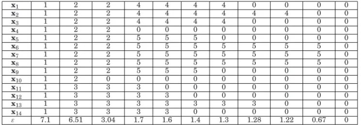
Let us consider a simple illustrative example involving the toy dataset in Figure 2. The application of HDBSCAN* to those data withmpts = 3 and Euclidean distance
results in the hierarchy shown in Table I. The relevant hierarchical levels in this case are those corresponding toε = 7.1, below which cluster C1 is split into C2 and C3,
ε=3.04, below which clusterC2is split intoC4andC5, andε=1.28, 1.22, and 0.67,
below which clustersC3,C4, andC5 disappear, respectively. In the remaining levels,
Table I. HDBSCAN* Hierarchy for the dataset in Figure 2, withmpts=3. Higher (lower) Hierarchical Levels are on the left (right). Values ofεin the Bottom row are those Assigned in Step 4.2.1 of Algorithm 1. The Remaining
Values are the labels Assigned in Steps 4.1 and 4.2.2: a non-null Valueiin thejth row Means that Objectxj
Belongs to ClusterCiat the Corresponding Level, Whereas a null Value Denotes Noise
x1 1 2 2 4 4 4 4 0 0 0 0 x2 1 2 2 4 4 4 4 4 4 0 0 x3 1 2 2 4 4 4 4 0 0 0 0 x4 1 2 2 0 0 0 0 0 0 0 0 x5 1 2 2 5 5 5 0 0 0 0 0 x6 1 2 2 5 5 5 5 5 5 5 0 x7 1 2 2 5 5 5 5 5 5 5 0 x8 1 2 2 5 5 5 5 5 5 5 0 x9 1 2 2 5 5 5 0 0 0 0 0 x10 1 2 0 0 0 0 0 0 0 0 0 x11 1 3 3 3 0 0 0 0 0 0 0 x12 1 3 3 3 3 0 0 0 0 0 0 x13 1 3 3 3 3 3 3 3 0 0 0 x14 1 3 3 3 3 0 0 0 0 0 0 ε 7.1 6.51 3.04 1.7 1.6 1.4 1.3 1.28 1.22 0.67 0
and C4, note that they are reduced to single objects in the intervals ε = [1.28 1.6)
andε=[1.22 1.3), respectively, before they completely disappear. This information is captured by the self-loops introduced in the extended MST, which describe the fact that
x13andx2become isolated, yet dense objects in the corresponding intervals.
ALGORITHM 2:HDBSCAN* Step 4.2.2 with (optional) parametermclSize≥1
4.2.2 After each removal (to obtain the next hierarchical level), process one at a time each cluster that contained the edge(s) just removed, by relabeling its resulting connected subcomponent(s):
Labelspurioussubcomponents as noise by assigning them the null label. If all subcomponents of a cluster arespurious, then thecluster has disappeared.
Else, if a single subcomponent of a cluster isnot spurious, keep its original cluster label (cluster has just shrunk).
Else, if two or more subcomponents of a cluster arenot spurious, assign new cluster labels to each of them (“true” cluster split).
The extended dendrogram that represents the density-based hierarchy in Table I is illustrated in Figure 3. Noise is indicated by thinner, red lines. The corresponding simplified cluster tree is displayed in Figure 4 (the values between parentheses in the nodes of the tree will be explained later). It is worth noticing that there are only five significant clusters in the tree, in contrast to 27 clusters that would exist in traditional hierarchical clusterings.
The idea for hierarchy simplification can be generalized by setting a minimum cluster size, a commonly used practice in real cluster analysis. In fact, in many practical applications of clustering (not just density-based clustering) a minimum cluster size is used as a user-specified parameter in order to prevent algorithms from finding very small clusters of objects that may be highly similar to each other just by chance, that is, as a consequence of the natural randomness associated with the use of a finite data sample (see, e.g., the notion of a particle in the work of Gupta et al. [2010]). Requiring a minimum cluster size,mclSize ≥1, allows only clusters with at leastmclSize
objects to be reported, and the case in which a component with fewer than mclSize
objects is disconnected from a cluster should not be considered as a “true” split. We can adapt HDBSCAN* accordingly by changing Step 4.2.2 of Algorithm 1, as shown
Fig. 3. Dendrogram corresponding to the HDBSCAN* hierarchy for the dataset in Figure 2, with mpts = 3 (hierarchy in Table I). Thinner, red lines denote noise.
Fig. 4. Cluster tree corresponding to the hierarchy in Table I. Numerical values within parentheses stand for the stability of the clusters according to their relative excess of mass.
in Algorithm 2: a connected component is deemedspuriousif it has fewer thanmclSize
objects or, formclSize =1, if it is an isolated, non-dense object (a vertex with no edges).
Any spurious component is labeled as noise. Cardinality check and labeling of the components can be trivially performed by a graph traversal procedure starting from the end vertices of the removed edge(s). In practice, this simplification procedure can reduce dramatically the number of clusters in the hierarchy.
Note that the optional use of the parametermclSize represents an additional,
inde-pendent control of the smoothing of the resulting cluster tree as a density estimate, in addition to the parametermpts. Note also that in the original definition of a
density-based cluster for DBSCAN Ester et al. [1996], mpts simultaneously acts as a direct
control of the minimum cluster size, sinceborderobjects (which we do not consider in HDBSCAN*) belong to the same clusters as their corresponding core objects; conse-quently, the resulting clusters have no fewer thanmptsobjects.5
To make HDBSCAN* more similar to previous density-based approaches like DB-SCAN in this respect, and also to simplify its use, we can setmclSize =mpts, which turns
mpts into a single parameter that acts at the same time as a smoothing factor of the
density estimates and an explicit threshold for the minimum size of clusters. 3.4. Computational Complexity
The asymptotic complexity of HDBSCAN* in Algorithms 1 and 2 is discussed in this section w.r.t. running time and memory space, considering two different scenarios. In the first scenario, the datasetXis available as an input to the algorithm. In the second (relational) scenario, the distance matrix Dis available instead. It is important to remark that one hasmpts n(where n = |X|) in any realistic application, so this
assumption is made here.
Let us first consider the first scenario, in whichXis available. We assume that the distanced(·,·) between any pair of objects can be computed in O(a) time—where a 5The DBSCAN algorithm, however, does not implement the possible multiple labels for border-objects but assigns a border object arbitrarily to just one of the clusters it belongs to.
is the number of attributes describing the objects—as usual for many dissimilarity functions. Then, in the most general case, Step 1 of the algorithm takes O(a n2) time,
as it demandsn K-NN queries (withK =mpts), one per each data object. By using a
simple implementation of Prim’s algorithm based on an ordinary list search (instead of a heap), it is possible to construct the MST in Step 2 of HDBSCAN* inO(n2+m) time,
where mis the number of edges of the mutual reachability graph (with nvertices). In the present context,m = n(n−1)/2 (complete undirected graph), so Step 2 runs in O(n2+m) → O(n2) time. Notice that it isnotnecessary to explicitly construct the
mutual reachability graph, as the mutual reachability distances (edge weights) can be computed on demand. In this case, the MST can be computed inO(a n2) time. The
number of edges in the MST is n−1, plus nadditional “self-edges” in the extended MST (Step 3). These 2n−1 edges need to be sorted so that Step 4 can be performed, which can be done inO(nlogn). After the sorting procedure, Step 4 reduces to a series of relabelings of smaller and smaller subcomponents of the MST. Notice that at most two subcomponents must be relabeled after each edge removal, and that spurious
components are never relabeled after they have become spurious. In the worst case, though, the whole relabeling procedure can still takeO(n2) time. In total, the overall
time complexity of the algorithm is thusO(a n2).
Still considering the first scenario, but now in terms of main memory requirements, it follows that one needs O(a n) space to store the dataset Xand O(n) space to store the core distances in Step 1 of the algorithm. In Steps 2 and 3, recall that the mutual reachability graph does not need to be explicitly computed, and only the edges of the resulting MSText must be stored, which requiresO(n) space. During the execution of
Step 4, only the hierarchical level being currently processed is needed at any point in time, which requires O(n) space. Therefore, the overall space complexity of the algorithm isO(a n).
In the case in which the distance matrixDis giveninsteadof the datasetX, the only change in terms of running time is that, as one can promptly access any distanced(·,·) fromDin constant time, the computations no longer depend on the dimensionaof the data space, and therefore the time complexity reduces toO(n2). On the other hand, this
requires that matrixDbe stored in main memory, which results inO(n2) complexity in
terms of space.
It is worth noticing that the running times discussed earlier can be reduced provided that some particular assumptions hold true, especially if the average case is considered. For instance, Step 1 of the algorithm can be computed in sub-quadratic time by using appropriate indexing structures for K-NN search in data spaces of low or moderate dimensionality. Even the MST in Step 2 might be computed (at least partially, as a forest) in sub-quadratic time, if an appropriate upper bound is imposed on the radius
ε, so that the mutual reachability graph becomes sparse (as in OPTICS [Ankerst et al. 1999]).
In terms of space, if one wants to keep the whole hierarchy in main memory (instead of iteratively saving each hierarchical level on disk as they are computed), the hierarchy does not need to be kept in its complete form illustrated in Table I. All the information one needs to recover the complete hierarchy is, for each data object, a list (set) of all cluster labels associated with that object along the hierarchy and the corresponding hierarchical levels (scales) at which the object first belongs to each of those clusters. Typically, all these lists together will be much smaller than a matrix as illustrated in Table I, specially for larger values ofmptsandmclSize.
Another alternative to optimize space is to store a compacted hierarchy containing only the most important hierarchical levels, namely, those in which the clusters in the cluster tree first appear or completely disappear. This can reduce significantly the size of the output file. A Java implementation of the algorithm that optionally supports this
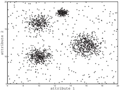
Fig. 5. Illustrative dataset with four clusters and background noise.
compaction strategy is available on request. As an example of this code’s performance, for a dataset with 50,000 objects distributed in 50 clusters in a 50 dimensional Eu-clidean space, the algorithm, running on a domestic laptop6, finished in 5.42 minutes and produced an output file of 14MB (containing the compacted hierarchy and the cluster tree).
4. VISUALIZATION
The HDBSCAN* hierarchy can be visualized in different ways, for example, as a den-drogram or simplified cluster tree, as illustrated in Figures 3 and 4, respectively. How-ever, while these plots can usually give a clear view of the cluster structure for small datasets, they may not be easy to read in more general application scenarios. Therefore, alternative forms of visualization may be needed.
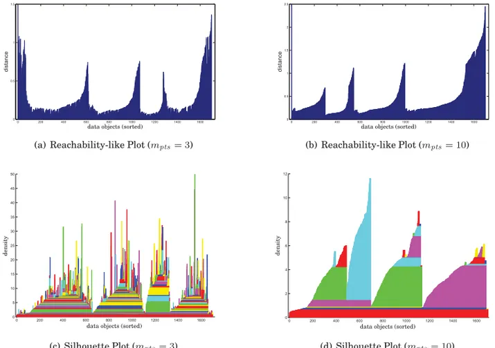
Ankerst et al. [1999] proposed the well-known OPTICS algorithm whose primary output is the so-calledreachability plot, which, roughly speaking, is a bar plot showing clusters as “dents” characterized by valleys and peaks along the bars. Sander et al. [2003] have shown that dendrograms in general (not necessarily density based) can be converted into, and visualized as, reachability-like plots. Provided that the data objects have already been sorted in the way they would be displayed in the dendrogram (i.e., with the objects in each cluster always placed next to each other), the basic idea is to plot a bar for each object whose height is the smallest dendrogram scale value at which the object gets merged into the same cluster as any of the preceding objects in the plot. For the HDBSCAN* hierarchy, an appropriate ordering in which objects in the same cluster necessarily appear next to each other when building the plot can be achieved by recursively sorting the subsets of objects in each cluster top-down the hierarchy, which is equivalent to a top-down level-wise lexicographic sorting according to the cluster labels.
As an illustrative example, let us consider the dataset in Figure 5, in which there are four clusters following 2D normal distributions and uniform background noise. The reachability-like plots corresponding to the HDBSCAN* hierarchies for these data with mpts = 3 and mpts = 10 are displayed in Figures 6(a) and 6(b), respectively. In
both figures, the four natural clusters appear clearly as the most prominent “dents”
6MacBook Pro, 2.5GHz Intel Core i5, 8GB RAM, Mac OS X Lion 10.7.5, running Java 7 with algorithm settings set tompts=mclSize=50.
Fig. 6. Reachability and silhouette plots of the HDBSCAN* hierarchy for the dataset in Figure 5, formpts=3 andmpts=10 (mclsize=mpts). Note that, since the clustering hierarchies are different for differentmpts, the sorting of the objects on the left- and right-hand figures are different.
in the plots, but formpts=10 the plot is smoother and subclusters do not show up as
apparently as formpts=3.
For density-based hierarchies, an alternative yet related form of visualization con-sists in sorting the data objects in the same way as in the reachability plots, but setting the height of each bar in the plot to the highest density such that the corresponding data object is still part of a cluster (not yet noise). This is in essence a type of dimensionless representation of a silhouette plot of densities [Muller and Sawitzki 1991]. Such a sil-houette plot can be made more sophisticated, as proposed by Gupta et al. [2010], by plotting in different colors the different segments of the bars that correspond to the density intervals along which an object belongs to different clusters in the hierarchy (each subcluster is assigned a particular color that is guaranteed to be different from its parent’s color). For the dataset in Figure 5, the silhouette plots of the HDBSCAN* hierarchies are illustrated in Figures 6(c) and 6(d). Formpts = 3 the plot is spikier and, from the changes in colors, it is clear that the hierarchy is more complex (many subclusters in the cluster tree). Formpts=10 the plot is smoother and we can see that the number of subclusters is drastically reduced.
Reachability or silhouette plots display hierarchical clusterings in different ways, but we can see from the example in Figure 6 that they both not only allow a visualization of the structure of clusters found by the algorithm, but also the effects of different settings of the algorithm on the clustering results. As such, these plots can be useful auxiliary tools for exploratory data analysis, particularly in the domain of unsupervised learning by means of the HDBSCAN* framework.
setting.
5.1. Cluster Stability
Without loss of generality, let us initially consider that the data objects are described by a single continuous-valued attributex. Recall from the introduction that, following Hartigan’s model [Hartigan 1975], the density-contour clusters of a given density f(x) onat a given density levelλare the maximal connected subsets of the level set defined as{x| f(x)≥ λ}. From Section 2, it follows that DBSCAN* estimates density-contour clusters using a density thresholdλ=1/εand a non-normalized K-NN estimate (for
K=mpts) of f(x), given by 1/dcore(x).7
HDBSCAN* produces all possible DBSCAN* solutions w.r.t. a given value ofmpts
and all thresholds λ = 1/ε in [0,∞). Intuitively, when increasingλ (i.e., decreasing
ε), clusters get smaller and smaller, until they disappear or break into subclusters. This observation gives rise to the intuition that, roughly speaking, more prominent clusters tend to “survive” longer after they appear, and which is essentially the rationale behind the definition ofcluster lifetimefrom classic hierarchical cluster analysis [Jain and Dubes 1988; Fred and Jain 2005]. The lifetime of a given cluster in a traditional dendrogram is defined as the length of the dendrogram scale along those hierarchical levels in which the cluster exists. In traditional dendrograms, however, the removal of a single object suffices to characterize the dissolution of a cluster and appearance of new ones, which makes the original definition inappropriate in the density-based context. Therefore, a different measure of stability is needed that considers the dissolution of a cluster under the broader perspective discussed in Section 3.3, which accounts for the presence of noise and spurious components along the hierarchy. Such a measure should also take into account the individual density profiles of the objects belonging to a cluster, that is, their possibly differentlifetimes as members of that cluster (before they become noise or members of another cluster).
To formalize the aforementioned idea, we adapt the notion ofexcess of mass[Muller and Sawitzki 1991], first introduced by Hartigan [1987] and more recently used in the context of estimates of level sets for continuous-valued PDF [Stuetzle and Nugent 2010]. Imagine increasing the density levelλand assume that a density-contour cluster
Ciappears at levelλmin(Ci), by definition as a maximal connected subset of the level set
{x| f(x)≥λmin(Ci)}. The excess of mass ofCiis defined in Equation (1), and illustrated in Figure 7, in which the darker shaded areas represent the excesses of mass of three
7From this perspective, the role ofm
ptsas a classic smoothing factor for such an estimate becomes clearer. It is worth remarking, however, that DBSCAN* does not attempt to produce a very accurate estimate of the true PDF of the data. The density estimate is used essentially to discriminate between noise and non-noise data objects, which contributes to makingmptsa particularly noncritical parameter.
Fig. 7. Illustration of a density function, clusters, and excesses of mass.
clusters, C3, C4, and C5. The excess of mass of C2 (not highlighted in the figure)
encompasses those of its childrenC4andC5.
E(Ci)=
x∈Ci
(f(x)−λmin(Ci))dx (1) Since the excess of mass of a cluster necessarily embodies those of all its descendants, this measure exhibits a monotonic behavior along any branch of the cluster tree. As a consequence, it cannot be used to compare nested clusters, such asC2againstC4and C5. To be able to do so, we introduce the notion ofrelative excess of massof a cluster Ci, which appears at levelλmin(Ci), as:
ER(Ci)=
x∈Ci
(λmax(x,Ci)−λmin(Ci))dx, (2) whereλmax(x,Ci)=min{f(x), λmax(Ci)}andλmax(Ci) is the density level at whichCi is split or disappears. For example, for clusterC2in Figure 7 it follows thatλmax(C2)=
λmin(C4)= λmin(C5). The corresponding relative excess of mass is represented by the
lighter shaded area in Figure 7.
For a HDBSCAN* hierarchy, in which we have a finite datasetX, cluster labels, and density thresholds associated with each hierarchical level, we can adapt Equation (2) to define thestabilityof a clusterCi as:
S(Ci)= xj∈Ci λmax(xj,Ci)−λmin(Ci) = xj∈Ci 1 εmin(xj,Ci)− 1 εmax(Ci) (3) where λmin(Ci) is the minimum density level at which Ci exists, λmax(xj,Ci) is the density level beyond which objectxj no longer belongs to clusterCi, andεmax(Ci) and
εmin(xj,Ci) are the corresponding values for the thresholdε.
Recalling the illustrative example described in Section 3.3, it follows that object
x11, for instance, belongs to clusterC3in the radius intervalε =[1.7 7.1), that is, in
the density interval λ = (1/7.1 1/1.7] = (0.14 0.59]. The first value of this density interval is preciselyλmin(C3), which is common to all objects of that cluster, namely, x11, x12, x13, and x14. The second value is λmax(x11,C3) = 0.59, above which x11 no
longer belongs to clusterC3. Analogously, it follows thatλmax(x12,C3)=λmax(x14,C3)=
1/1.6=0.625 andλmax(x13,C3)=1/1.28=0.781. Thence, the relative excess of mass
of clusterC3 according to Equation (3) isS(C3)=2.06. The relative excesses of mass
for the other clusters are displayed in the nodes of the cluster tree in Figure 4. The value for the rootC1is not shown to emphasize thatC1, which represents the whole
5.2. Optimization Algorithm for Unsupervised Cluster Extraction
Let{C2, . . . ,Cκ}be the collection of all clusters in the simplified cluster hierarchy (tree)
generated by HDBSCAN*, except the rootC1, and letS(Ci) denote the stability value of each cluster. The goal is to extract the most “prominent” clusters (plus possibly noise) as a flat, nonoverlapping clustering solution. This task can be formulated as an opti-mization problem with the objective of maximizing the overall aggregated stabilities of the extracted clusters, in the following way:
max δ2, ... ,δκ J= κ i=2 δiS(Ci) subject to δi ∈ {0,1}, i=2, . . . , κ
exactly oneδ(·)=1 in each path from a leaf cluster to the root
(4)
whereδi indicates whether clusterCi is included into the flat solution (δi =1) or not (δi =0). The constraints imposed on the decision variablesδ2, . . . , δκ prevent clusters
on the same branch of the tree to be simultaneously selected; clearly, for inclusion in a flat solution, nested clusters must be mutually exclusive, that is, each object can only be assigned a single label.
To solve Problem (4) both globally and efficiently, we notice that the subselection of clusters in any subtree of the cluster tree represents a subproblem of the very same nature of the original problem (i.e., the one that refers to the complete tree). From this observation, a dynamic programming strategy can be applied that incrementally solves subproblems (subtrees) of increasing sizes, starting from the leaves and aggre-gating the intermediate solutions upwards in the tree. Specifically, we process every node except the root, starting from the leaves (bottom-up), deciding at each nodeCi whetherCi or the best-so-far selection of clusters inCi’s subtrees should be selected. To be able to make this decision locally atCi, we propagate and update the total sta-bility ˆS(Ci) of clusters selected in the subtree rooted atCi in the following, recursive way:
ˆ
S(Ci)=
S(Ci), ifCi is a leaf node max{S(Ci),Sˆ(Cil)+Sˆ(Cir)} ifCi is an internal node
(5) whereCil and Cir are the left and right children ofCi (for the sake of simplicity, we discuss the case of binary trees; the generalization ton-ary trees is trivial).
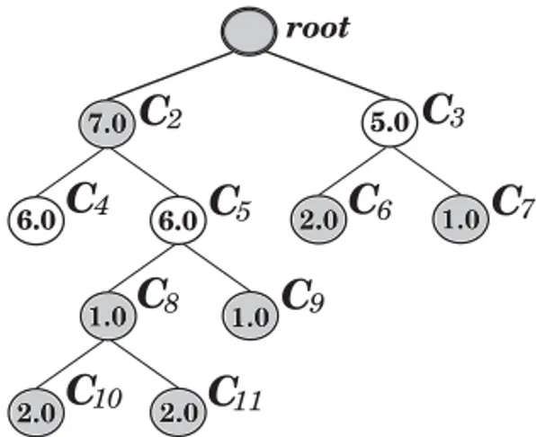
Fig. 8. Illustration of the optimal selection of clusters from a given cluster tree.
Algorithm 3 gives the pseudocode for finding the optimal solution to Problem (4). Figure 8 illustrates the algorithm. ClustersC10andC11 together are better thanC8,
which is then discarded. However, when the set{C10,C11,C9}is compared toC5, they
are discarded as C5 is better. Clusters {C4} and {C5} are better than C2, and C3 is
better than{C6,C7}, so that in the end, only clustersC3,C4, andC5remain, which is
the optimal solution to Problem (4) withJ=17.
ALGORITHM 3:Solution to Problem (4)
1. Initializeδ2= · · · =δκ=1, and, for all leaf nodes, set ˆS(Ch)=S(Ch).
2. Starting from the deepest levels, do bottom-up (except for the root): 2.1 IfS(Ci)<Sˆ(Cil)+Sˆ(Cir), set ˆS(Ci)=Sˆ(Cil)+Sˆ(Cir) and setδi=0.
2.2 Else: set ˆS(Ci)=S(Ci) and setδ(·)=0 for all clusters inCi’s subtrees.
Notice that Step 2.2 of Algorithm 3 can be implemented in a more efficient way by not settingδ(·) values to 0 for discarded clusters down in the subtrees (which could happen
multiple times for the same cluster). Instead, in a simple postprocessing procedure, the tree can be traversed top-down in order to find, for each branch, the shallowest cluster that has not been discarded (δ(·)=1). Thus, Algorithm 3 can be implemented with two
traversals through the tree, one bottom-up and another one top-down. This results in an asymptotic complexity of O(κ), both in terms of running time and memory space, whereκ is the number of clusters in the simplified cluster tree, which is O(n) in the worst case.
5.3. Semisupervised Cluster Extraction
In many different application scenarios, a certain, usually small amount of information about the data may be available that allows one to perform clustering in a semisu-pervised rather than in a completely unsusemisu-pervised way. The most common type of information appears in the form of instance-level constraints, which encourage pairs of objects to be grouped together in the same cluster (should-link constraints) or to be separated apart in different clusters (should-not-link constraints) [Wagstaff 2002; Basu et al. 2008]. These areexternal,explicitconstraints provided by the user or analyst in
additionto theinternal,implicitconstraints that follow from the inductive bias of the clustering model that has been adopted.
instance-level constraints is rather straightforward by noticing that we can replace the values of stability for each cluster,S(Ci), with the fraction of constraints that are satisfied by that cluster,(Ci) = 21nc xj∈Ciγ(xj,Ci), wherenc is the total number of available constraints andγ(xj,Ci) is the number of constraintsinvolving objectxjthat are satisfied (not violated) ifCi is selected as part of the final flat solution. The scaling constant1/
2in(Ci) is due to the fact that a single constraint involves a pair of objects and, as such, it is taken into account twice in the sum. Term(Ci) is zero for clusters whose objects are not involved in any constraints.
Merely replacingS(Ci) with(Ci), however, would not account for the fact that some objects may not belong to any of the selected clusters, that is, they may be labeled as noise in the final flat solution. For example, let us recall the toy problem illustrated in Section 3.3. In particular, let us consider a candidate flat solution given by{C3,C4,C5}.
From the hierarchy in Table I it can be seen that objectx4, for instance, belongs to
none of these clusters. It belongs toC2and becomes noise at the same density level as
this cluster is split intoC4 and C5. Something similar is observed w.r.t.x10. Objects x4andx10 would therefore be labeled as noise in a flat solution composed of clusters C3,C4, andC5. Notice that since a noise object is, by definition, not clustered with any
other object, a should-not-link constraint involving one or both objects labeled as noise must be deemed satisfied, while a should-link constraint must be deemed violated. Noise objects, therefore, also affect the degree of satisfaction/violation of constraints, and thus they cannot be dismissed.
In order to account for the noise, we keep track of objects that are part of a cluster but not part of its subclusters in the hierarchy (if any). This information can be rep-resented by means of“virtual” nodes in the simplified cluster tree. We assume that every internal node of the cluster tree has one such virtual child node, even though only some of them may actually be associated with noise objects. The virtual child node of a clusterClin the cluster tree will be denoted hereafter asC∅l. We then define
(C∅l) = 21n
c xj∈C∅l γ(xj,C ∅
l) as the fraction of constraint satisfactions involving the noise objects associated withC∅l (which is zero if no noise object is associated withCl∅). For example, consider again the hierarchy in Table I and assume that the user has provided three should-link constraints, (x1,x5), (x3,x9), and (x2,x6), and a single
should-not-link constraint, (x7,x10). The internal nodes areC1andC2. Since there is no
noise object in the virtual node of the root,C∅1, it follows that(C∅1)=0. The noise objects inC∅2arex4andx10, but there is no constraint involving objectx4, thenγ(x4,C∅2)=0.
The only constraint involving objectx10is satisfied inC∅2, that is,γ(x10,C∅2)=1 (because x10, as noise, is not grouped with x7). Therefore, (C∅2) =
1
2×4(0+1) = 1