Applications
A THESIS
SUBMITTED TO THE FACULTY OF THE GRADUATE SCHOOL OF THE UNIVERSITY OF MINNESOTA
BY
Han-Tai Shiao
IN PARTIAL FULFILLMENT OF THE REQUIREMENTS FOR THE DEGREE OF
DOCTOR OF PHILOSOPHY
Vladimir S. Cherkassky, Advisor
First of all, I would like to express my deepest thanks to my advisor, Professor Vladimir Cherkassky, who guided me through my graduate study and research work.
He has always skillfully moved between letting me figure things out myself, and pointing me in the right direction. I sincerely appreciate his advice and consistent encouragement.
I would also like to thank my Ph.D. committee members, Professor Jarvis Haupt, Professor Mingyi Hong, and Professor Wei Pan, for reviewing my thesis and giving valuable feedback on my work.
I thank my former and current colleagues in our lab, Dr. Feng Cai, Dr. Sauptik Dhar, Jieun Lee, Thomas Vacek, Adarsh Sivasankaran, Brandon Veber, Hsiang-Han Chen, Zhong Zhuang, and many others for their help and friendship.
Special thanks to Adarsh who generously offered his time for proofreading my draft. Special thanks to Dr. Dan Drake, an alumnus of University of Minnesota. He gave me the style files and skeleton of his thesis so that I can typeset my thesis in LATEX easily.
Finally, I shall express my appreciation to my friends and families, for their assistance and encouragements over the years. Particularly, I appreciate the supports from my parents and parents-in-law.
To my wife Ya-Yin.
There has been a dramatic increase in application of statistical and machine learning methods for predictive data-analytic modeling of biomedical data. Most existing work in this area involves application of standard supervised learning techniques. Typical methods include standard classification or regression techniques, where the goal is to es-timate an indicator function (classification decision rule) or real-valued function of input variables, from finite training sample. However, real-world data often contain additional information besides labeled training samples. Incorporating this additional information into learning (model estimation) leads to nonstandard/advanced learning formalizations that represent extensions of standard supervised learning. Recent examples of such ad-vanced methodologies include semi-supervised learning (or transduction) and learning through contradiction (or Universum learning).
This thesis investigates two new advanced learning methodologies along with their biomedical applications. The first one is motivated by modeling complex survival data which can incorporate future, censored, or unknown data, in addition to (traditional) labeled training data. Here we propose original formalization for predictive modeling of survival data, under the framework of Learning Using Privileged Information (LUPI) proposed by Vapnik [1, 2]. Survival data represents a collection of time observations about events. Our modeling goal is to predict the state (alive/dead) of a subject at a pre-determined future time point. We explore modeling of survival data as binary classification problem that incorporates additional information (such as time of death, censored/uncensored status, etc.) under LUPI framework. Then we propose two ad-vanced constructive Support Vector Machine (SVM)-based formulations: SVM+ and Loss-Order SVM (LO-SVM). Empirical results using simulated and real-life survival data indicate that the proposed LUPI-based methods are very effective (versus classical Cox regression) when the survival time does not follow classical probabilistic assumptions.
Second advanced methodology investigates a new learning paradigm for classification called Group Learning. This approach is motivated by modeling high-dimensional data when the number of input features is much larger than the number of training samples. There are two main approaches to solving such ill-posed problems: (a) selecting a small number of informative features via feature selection; (b) using all features but imposing additional complexity constraints, e.g., ridge regression, SVM, LASSO, etc. The pro-posed Group Learning method takes a different approach, by splitting all features into many (t) groups, and then estimating a classifier in reduced space (of dimensionality d/t). This approach effectively uses all features, but implements training in a lower-dimensional input space. Note that the formation of groups reflects application-domain knowledge. For example, in classifying of two-dimensional images represented as a set of pixels (original high-dimensional input space), appropriate groups can be formed by grouping adjacent pixels or “local patches” because adjacent pixels are known to be highly correlated. We provide empirical validation of this new methodology for two real-life applications: (a) handwritten digit recognition, and (b) predictive classification of univariate signals, e.g., prediction of epileptic seizures from intracranial electroen-cephalogram (iEEG) signal. Prediction of epileptic seizures is particularly challenging, due to highly unbalanced data (just 4–5 observed seizures) and patient-specific modeling. In a joint project with Mayo Clinic, we have incorporated the Group Learning approach into an SVM-based system for seizure prediction. This system performs subject-specific modeling and achieves robust prediction performance.
Acknowledgments i
Dedication ii
Abstract iii
List of Figures vii
List of Tables ix
Chapter 1. General Introduction 1
1.1. Motivations 1
1.2. Technical Contributions 2
1.3. Structure of the Thesis 3
Chapter 2. Background 5
2.1. Objective of Predictive Learning 5
2.2. Classification 6
2.3. SVM for Classification 6
2.4. Nonlinear SVM 11
Part 1. Extensions of LUPI 13
Chapter 3. Learning Using Privileged Information 14
3.1. Introduction 14 3.2. SVM+ 17 3.3. Loss-Order SVM 30 3.4. SVM+ versus Loss-Order SVM 34 3.5. Summary 34 v
Chapter 4. Modeling of Survival Data 36
4.1. Introduction 36
4.2. Survival Analysis 39
4.3. Problem Formalization 47
4.4. Modeling of Survival Data 48
4.5. Empirical Comparisons 54
4.6. Summary 65
Part 2. Group Learning 67
Chapter 5. Overview 68
Chapter 6. Group Learning for Images 73
6.1. Introduction 73
6.2. Problem Formalization 74
6.3. Qualitative Analysis 76
6.4. Empirical Results 78
6.5. Summary 81
Chapter 7. Group Learning for One-Dimensional Signals 83
7.1. Introduction 83
7.2. Problem Formalization 85
7.3. Feature Engineering 88
7.4. SVM System and Experimental Design 91
7.5. Postprocessing 96
7.6. Empirical Evaluation 99
7.7. Summary 103
2.1 Binary classification problem. 8
2.2 Nonseparable case for binary classification. 10
3.1 SVM+ maps the training data into different spaces. 18
3.2 An arbitrary linear correcting function would violates ξ(x∗)≥0. 21 3.3 The only two valid linear correcting functions ifx∗ is bounded. 22
3.4 Nonlinear correcting functions. 23
3.5 Estimates of computational time of SVM+ implemented in CVX. 25
3.6 Illustration of the enforcing of ordering in LO-SVM. 33
4.1 Example of survival data in a calendar-time scale. 40
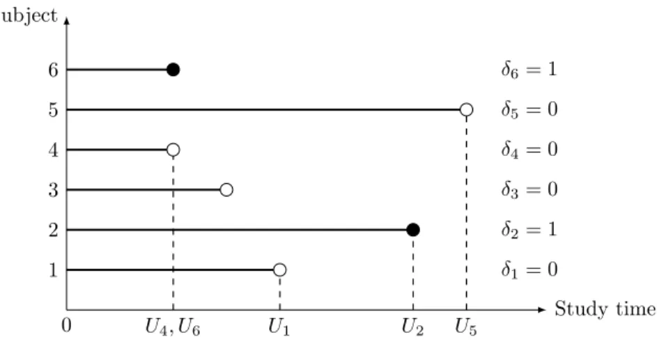
4.2 Example of survival data in a study-time scale. 41
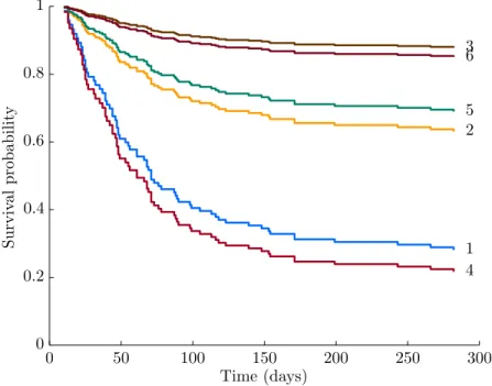
4.3 Estimated survival functions based on Cox model. 46
4.4 Example of survival data under the predictive problem setting. 48
4.5 Using Cox model in the predictive setting 50
4.6 The certainty measures for exact and censored observations. 51
4.7 The univariate privileged informationx∗ for LO-SVM. 52 4.8 Histograms of projections for training data with different noise levels. 56
5.1 MNIST digits 5 and 8 of size 28×28 pixels. 70
5.2 Partition digit 5 into four nonoverlapping patches of size 14×14 pixels. 71
5.3 Partition digit 8 into four nonoverlapping patches of size 14×14 pixels. 71
6.1 Illustration of Standard machine learning approach. 75
6.2 Illustration of Group Learning approach. 75
6.3 Training errors for standard SVM and Group Learning (patches 14-by-14). 79
6.4 Test errors for standard SVM and Group Learning (patches 14-by-14). 80
6.5 MNIST digit 5 and 8 of size 10×10 pixels. 81
6.6 Training errors for standard SVM and Group Learning (patches 10-by-10). 81
6.7 Test errors for standard SVM and Group Learning (patches 10-by-10). 82
7.1 Three feature encodings for iEEG data: BFB, FFT, and XCORR. 90
7.2 Proposed system design for training stage. 91
7.3 Proposed system design for prediction stage. 91
7.4 Predictive modeling in three time scales: 20 s, 1 hr, and 4 hr. 93
7.5 Histograms of Projections of SVM model for Dog-L4 training data. 96
7.6 Histograms of Projections of SVM model for Dog-L4 test data. 98
7.7 Univariate histogram of projections for test samples (a). 99
4.1 Test errors as a function of training sample size 57
4.2 Test errors as a function of censoring rate 58
4.3 Test errors as a function of noise level in survival time 59
4.4 Test errors as a function of training sample size without censored data 60
4.5 Summary of the statistical properties of survival datasets 62
4.6 Experimental results for survival datasets: linear models 63
4.7 Experimental results for survival datasets: nonlinear models 64
7.1 The number of interictal/preictal 1 hr segments for each dog 89
7.2 Experimental design for Dog-L4 under the unbalanced Setting 94
7.3 Predictions for 1 hr and 4 hr segments via different feature encodings 101
7.4 Summary of prediction performances on FP and FN error rates (%) 102
7.5 Summary of prediction performances on SS (%) and FPR per day 102
General Introduction
1.1. Motivations
Learning is the process of estimating an unknown (input, output) dependency from a limited number of observations [3, 4]. Various applications in engineering, statistics, computer science, health sciences, and social sciences are concerned with estimating “good” predictive models from the available historical data (or training data), in order to use this model for predicting future samples (or test data). Predictive learning is of particular interest because it can objectively define the “usefulness” of the estimated model by predictive (generalization) capabilities.
Most existing work on predictive data analytics involves development and applica-tion of standard supervised learning techniques. Typical methods include standard clas-sification or regression techniques, where the goal is to estimate an indicator function (classification decision rule) or real-valued function of input variables, from finite training sample. However, real-world data often contains additional information (besides labeled training samples). Incorporating this additional information into learning (model estima-tion) leads to non-standard/advanced learning formalizations that represent extensions of standard supervised learning. Recent examples of such advanced methodologies in-clude semi-supervised learning (or transduction) and learning through contradiction (or Universum learning). This thesis investigates two new advanced learning methodologies along with their biomedical applications.
The first contribution is a new mathematical formalization for modeling survival data which can incorporate future, censored, or unknown data, in addition to (tra-ditional) labeled training data. Here we propose original formalization for predictive
modeling of survival data, under the framework of Learning Using Privileged Informa-tion (LUPI) proposed by Vapnik [1, 2]. Survival data represents a collection of time observations about events. Our modeling goal is to predict the state (alive/dead) of a subject at a pre-determined future time point. We explore modeling of survival data as binary classification problem that incorporates additional information (such as time of death, censored/uncensored status, etc.) under LUPI framework. Then we propose two advanced constructive Support Vector Machine (SVM)-based formulations: SVM+ and Loss-Order SVM (LO-SVM). Empirical results using simulated and real-life survival data indicate that the proposed LUPI-based methods are very effective (versus classical Cox regression) when the survival time does not follow classical probabilistic assumptions.
Our second technical contribution is a new learning method for classification called Group Learning. This method is motivated by modeling high-dimensional data when the number of input features is much larger than the number of training samples. There are two main approaches to solving such ill-posed problems: (a) selecting a small number of informative features via feature selection; (b) using all features but imposing additional complexity constraints, e.g., ridge regression, SVM, LASSO, etc. The proposed Group Learning method takes a different approach, by splitting all features into several (t) groups, and then estimating a classifier in reduced space (of dimensionality d/t). This approach effectively incorporates all input features, but implements training in a lower-dimensional input space. Note that the formation of groups reflects application-domain knowledge. For example, for classification of two-dimensional (2-D) images represented as a set of pixels (original high-dimensional input space), appropriate groups can be formed by grouping adjacent pixels or “local patches” because adjacent pixels are known to be highly correlated. We provide empirical validation of this new methodology for two real-life applications (a) handwritten digit recognition, and (b) predictive classification of univariate signals, e.g., prediction of epileptic seizures from intracranial electroen-cephalogram (iEEG) signal.
1.2. Technical Contributions
• For modeling survival data:
(1) We demonstrated application of SVM+, a LUPI-based learning method, for modeling survival data under binary classification setting. This approach incorporates the survival time information into learning and can also handle censored observations.
(2) We proposed LO-SVM algorithm under LUPI framework. This LO-SVM can encode the survival time information effectively via a new ordering mechanism. We provided empirical comparisons between SVM+, LO-SVM, standard LO-SVM, and statistical model for survival data.
• For Group Learning method:
(1) We developed a Group Learning framework for modeling high-dimensional data under classification setting. The proposed learning methodology has been shown empirically its effectiveness in application of 2-D image recog-nition problems.
(2) We provided an application of Group Learning to seizure prediction prob-lems formalized as classification of univariate signals (i.e., iEEG recordings of brain activity). Empirical results show that the proposed seizure pre-diction system achieves high sensitivity and low false-positive error rate.
1.3. Structure of the Thesis
This thesis includes three major parts:
(1) Background description of predictive learning and SVM (in Chapter 2). (2) Extensions of LUPI for modeling survival data (Chapters3 and 4).
(3) Group Learning with application to prediction of epileptic seizures (Chapters5,
6, and7).
Part I on modeling survival data is based on the following publications and manu-script:
• H.-T. Shiao and V. Cherkassky, “Learning Using Privileged Information (LUPI) for modeling survival data,” in Neural Networks (IJCNN), 2014 International Joint Con-ference on, Jul. 2014.
• H.-T. Shiao, T. Vacek, and V. Cherkassky, “LUPI-based approaches for modeling survival data,” in Proceedings of the International Workshop on Human is More Than a Labeler (BeyondLabeler), co-located with the 25th International Joint Conference on Artificial Intelligence (IJCAI 2016), Jul. 2016.
• H.-T. Shiao, T. Vacek, and V. Cherkassky, “Predictive modeling of survival data,” submitted to IEEE Trans. Neural Netw. Learn. Syst., under review.
Part IIon Group Learning is based on the following publications and manuscript:
• V. Cherkassky, B. Veber, J. Lee, H.-T. Shiao, E. Patterson, G. A. Worrell, and B. H. Brinkmann, “Reliable seizure prediction from EEG data,” in Neural Networks (IJCNN), 2015 International Joint Conference on, Jul. 2015.
• H.-T. Shiao, V. Cherkassky, J. Lee, B. Veber, E. Patterson, B. H. Brinkmann, and G. A. Worrell, “SVM-based system for prediction of epileptic seizures from iEEG sig-nal,”IEEE Trans. Biomed. Eng., vol. 64, pp. 1011–1022, May 2017.
• H.-T.Shiao, V. Cherkassky, “Group Learning: shallow deep learning,” in preparation.
• H.-H. Chen, H.-T. Shiao, V. Cherkassky, “Online prediction system for epileptic seizures using iEEG signal,” in preparation.
Background
This chapter reviews the basic concepts of predictive learning and Support Vector Machine (SVM). The content of this chapter mainly follows [3, 4, 5].
2.1. Objective of Predictive Learning
The process of learning is about estimating an unknown dependency or structure between the input and output of a system, based on a limited number of observations. The finite training set is denoted as independent identically distributed pairs
(x1, y1), . . . ,(xn, yn), (2.1)
generated from a fixed but unknown probability measureP(x, y). Supposef(x, ω) denote the set of functions estimated by the learning machine and indexed byω. The quality of an approximation produced by the learning machine is measured by the lossL(f(x, ω), y), or the discrepancy between the outputyproduced by the original system and the output f(x, ω) produced by learning machine for a given input x.
The goal of learning is to estimate the functionf(x, ω0) that guarantees the smallest loss. That is, the goal is to find the function which minimizes therisk functional
R(ω) =
Z Z
L(f(x, ω), y)P(x, y) dxdy (2.2)
over the set of functions supported by the learning machine using only training data (2.1). With finite data we cannot expect to find f(x, ω0) exactly. Instead, we can obtain
f(x, ω∗) which represents the estimate of the optimal solution obtained with finite
train-ing data ustrain-ing one learntrain-ing procedure. The estimated function f(x, ω∗) is expected
to have good prediction accuracy for future (test) data. High prediction accuracy is normally called goodgeneralization in the field of machine learning.
In practice, in order to evaluate a machine learning algorithm or compare different algorithms, we use the so called test error as the criteria. Suppose we are given a test set (xj, yj), j= 1, . . . , m, the test error is defined as
Etest= m X j=1 L(f(xj, ω∗), yj). (2.3) 2.2. Classification
For the generic learning problems, classification and regression are two common learning tasks. The differences between classification and regression are the outputs and loss functions. We will mainly deal with binary classification in this thesis.
The output of a binary classification system takes on only two valuesy ∈ {+1,−1}
corresponding to two classes. Hence, in learning machine, f(x, ω), ω ∈ Ω, are a set of indicator functions. The most commonly used loss function for binary classification problem is the misclassification error defined as
L(f(x, ω), y) = 0, ify=f(x, ω), 1, ify6=f(x, ω).
For completeness, we also give a brief description about regression here. The output of the system in a regression problem takes on real values: y∈R. In a learning machine, f(x, ω), ω ∈ Ω, are a set of functions with real values. A common loss function for regression problem is the squared error defined as
L(f(x, ω), y) = (y−f(x, ω))2.
2.3. SVM for Classification
This section describes a family of learning algorithms known as Support Vector Ma-chine and provides the fundamental mathematical formulation of SVM. SVM method-ology was developed in Statistical Learning Theory [6], and later was adopted by re-searchers in machine learning, statistics, and signal processing.
According to Vapnik-Chervonenkis (VC) theory, the generalization bound for learn-ing with finite samples is as follows,
R(ω)≤Remp(ω) + Φ h n, logη n . (2.4)
Detailed analysis suggests that the second term Φ, called theconfidence interval, depends mainly on the VC-dimension (or the ratio h/n), whereas the first term (empirical risk) depends on parameter ω. SVM provides a special way to achieve small empirical risk (first term) using low complexity (second term) parameterizations. Therefore, SVM provides good generalization for future (test) data.
Consider a binary classification setting where we are given finite training data (xi, yi),
i = 1, . . . , n, with x ∈ Rd and y ∈ {+1,−1}. The goal of SVM is to find the optimal decision function
f(x) = sgn(w,x) +b
with good generalization performance.
Assuming that training data is linearly separable, there are many separating hyper-planes (w,x) +bsatisfying the constraints
yi((w,xi) +b)≥1,
for i = 1, . . . , n. SVM method considers an optimal separating hyperplane, for which the margin (i.e., the distance between the closest data points to the hyperplane) is maximized [6, 7]. The VC dimension (model complexity) of an optimal separating hyperplane is h≤min r2 ∆2, d + 1, (2.5)
where r is the radius of the smallest sphere that contains the training input vectors (x1, . . . ,xn), and ∆ is the margin. SVM implements structural risk minimization (SRM)
inductive principle by keeping the value of empirical risk fixed (zero for the linearly separable case) and minimizing the confidence interval (by maximizing margin). The concept of margin is illustrated in Figure 2.1.
f(x) = 0 +1 −1 1/kwk y= +1 y =−1
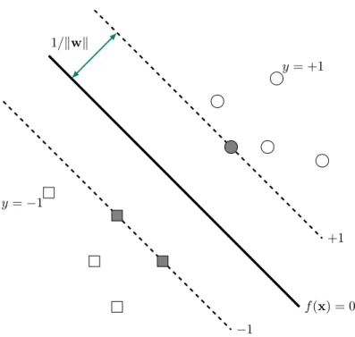
Figure 2.1. Binary classification problem, where circles denote samples
from positive class and squares denote samples from negative class. The margin 1/kwk is the distance between the closest data points to the hy-perplane. The shaded circle(s) and square(s) represent the support vec-tors.
Maximization of margin is equivalent to minimization of kwk. To this end, SVM solves the following optimization problem:
minimize 1 2kwk
2
subject to yi((w,xi) +b)≥1, i= 1, . . . , n,
(2.6)
with w ∈ Rd and b ∈ R as the variables. That is, the problem of finding an optimal large-margin separating hyperplane for linearly separable data is reduced to a quadratic programming (QP) problem (2.6). It is common to solve (2.6) (the primal problem) in its dual form. According to convex optimization, an optimization problem has a dual form if the objective function and constraints are strictly convex [8]. In this case, solving
the dual problem is equivalent to solving the original. The dual form of (2.6) is maximize n X i=1 αi− 1 2 n X i=1 n X j=1 αiαjyiyj(xi,xj) subject to n X i=1 αiyi= 0, α0, (2.7)
withα∈Rn+ as the variables. The optimal hyperplane decision function has the follow-ing form f(x) = n X i=1 α∗iyi(x,xi) + ˆb, (2.8) whereα∗
i,i= 1, . . . , n, are the solutions of (2.7), and ˆbis called the bias term.
The parameters αi are generally known as Lagrange multipliers. Note that αi ≥0
correspond to the constraints yi((w,xi) +b) ≥ 1 in (2.6). That is, data points that
satisfy the constraints with inequality have their multipliers in (2.8) equal zero. The data points that satisfy the constraints withequality are support vectors, and they have nonzero values of α∗
i. Therefore, the solution (2.8) depends only on a subset of data
points, i.e., support vectors. The support vectors are illustrated in Figure 2.1 with shaded circle(s) and square(s). Once the Lagrange multipliers have been estimated, the bias term ˆbcan be calculated using any of the support vectors (xs, ys):
ˆb=ys−
n
X
i=1
α∗iyi(xs,xi). (2.9)
When training data are not linearly separable, the empirical risk Remp(w) is no longer zero. That is, a few training samples are allowed to fall inside the margin (so called soft margin). One can introduce the nonnegative slack variables
ξi = max(1−yif(xi,w),0), (2.10)
for i= 1, . . . , n, to represent the deviations from margin borders, as illustrated in Fig-ure2.2. The empirical risk is then defined as
Remp(w) =
n
X
i=1
In this case, SVM attempts to strike a balance between the goal of empirical risk mini-mization and margin maximini-mization by solving the following optimini-mization problem:
minimize 1 2kwk 2+C n X i=1 ξi subject to yi((w,xi) +b)≥1−ξi, i= 1, . . . , n, ξ 0, (2.11)
withw∈Rd,b∈R, andξ ∈Rn+ as the variables.
f(x) = 0 +1 −1 1/kwk ξ1 ξ2 ξ3 x1 x2 x3 y= +1 y =−1
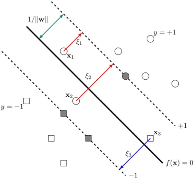
Figure 2.2. Nonseparable case for binary classification. Slack variables ξi = 1−yif(xi) correspond to the deviation from the margin borders.
Three data pointsx1,x2, andx3 are nonseparable, since they are within the margin. Data points x2 and x3 are misclassified, since they are on the wrong side of the decision boundary. Data pointx1 is nonseparable, but classified correctly.
Thekwk term in the objective function of (2.11) controls the size of margin. Theξi
(xi, yi). The parameter C, selected by users, controls the trade-off between the
com-plexity and proportion of nonseparable samples. The selection of C is known as model selection, and it is usually done via cross validation.
Problem (2.11) is also solvable in its dual form:
maximize n X i=1 αi− 1 2 n X i=1 n X j=1 αiαjyiyj(xi,xj) subject to n X i=1 αiyi= 0, 0αC, (2.12)
with α ∈ Rn+ as the variables. This optimization problem differs from that for the separable case (2.7) only with the inclusion of a maximum limitCin constraints. So (2.7), for linearly separable data, can be regarded as a special case of (2.12) with a very large value of parameter C. The optimal hyperplane decision function has the same form as for the separable case (2.8):
f(x) = n X i=1 α∗iyi(x,xi) + ˆb, whereα∗
i,i= 1, . . . , n, are the solutions of (2.12) and the bias ˆbis given in (2.9).
2.4. Nonlinear SVM
This section discuss how to construct large margin nonlinear decision boundary. The general approach is to map the input vectorxinto a high-dimensional feature space, and then construct an optimal hyperplane in this feature space [4,6]. Obviously, hyperplanes in this feature space will correspond to nonlinear decision boundaries in the input space. The conceptual motivation for the nonlinear mapping can be also provided by the VC generalization bound (2.4). Note that the empirical risk term in (2.4) can be always reduced to zero or a small value following the nonlinear mapping Ψ(x) :x7→zto a high-dimensional feature space. So a good generalization may be guaranteed, if the confidence interval Φ is small, which can be achieved by controlling the VC dimension, i.e., using large margin hyperplanes in the feature space.
To extend the linear SVM to a nonlinear one, we do not need to specify the nonlinear basis function Ψ explicitly. It is sufficient to provide a kernel function K(xi,xj) in the
input space and substitute the dot product (xi,xj) in (2.7), (2.8), (2.9), and (2.12) with
K(xi,xj). Hence, the nonlinear version of (2.12) is
maximize n X i=1 αi−1 2 n X i=1 n X j=1 αiαjyiyjK(xi,xj) subject to n X i=1 αiyi = 0, 0αC, (2.13)
and the nonlinear SVM decision function is
f(x) =
n
X
i=1
α∗iyiK(x,xi) + ˆb, (2.14)
with the bias term
ˆ b=ys− n X i=1 α∗iyiK(xs,xi). (2.15)
The kernel function K(xi,xj) effectively defines the (nonlinear) similarity metric
between any two data points xi and xj in the input space. Commonly used kernel
functions include:
(1) Polynomial kernel of degree m (wherem is a positive integer)
K(xi,xj) = ((xi,xj) + 1)m.
(2) Radial basis function (RBF) kernel with width parameterσ
K(xi,xj) = exp −kxi−xjk 2 2σ2 , or in alternative form K(xi,xj) = exp −γkxi−xjk2, with γ >0.
Learning Using Privileged Information
This chapter describes a learning paradigm called Learning Using Privileged Informa-tion (LUPI), a general methodology for utilizing addiInforma-tional informaInforma-tion about training data. Two mathematical formulations under the LUPI framework, namely SVM+ and Loss-Order SVM, are introduced in this chapter as well.3.1. Introduction
In a data-rich world, there often exists additional information about training data, which is not reflected in the labeled training samples (xi, yi),i= 1, . . . , n. This additional
information is not known during prediction, so the goal of learning is to estimate a model ˆ
y=f(x), as in standard inductive learning [4].
We use the following examples to illustrate this possibility.
(1) Handwritten digit recognition, whereas the training data are known to be gen-erated by several persons. In this case, each training sample has an additional person (group) label, and this information can be used to improve generaliza-tion. However, this group label is not available during the test stage, e.g., a classifier uses only pixels of an image for making prediction.
(2) Medical diagnosis, whereas the goal is to estimate a predictive classifier for di-agnosing a disease based on the clinical tests, or input features x, known at the time of initial examination. However, the available data may include addi-tional patient history obtained later, such as pathological reports and advanced tests. This additional information, denoted as feature vector x∗, can be used for training a classifier. However, features x∗ are not known during testing (or
prediction stage of a classifier). Hence, the goal of learning is to estimate a
decision rule ˆy =f(x), a function of input features only known at the time of initial examination.
(3) Time series prediction, whereas the goal is to predict a future event based on past (known) values of a time series. For instance, given historical information about the values of a stock market index up to moment t, we would like to predict if this index at moment t+δtwill be higher or lower (roughly speaking to make a decision to sell or buy). Clearly, the historical data (used for training) also includes the values of the index around t+δt, e.g., two days before and after t+δt. This additional information can be incorporated into training, and it may improve generalization.
All these examples include potentially useful extra information about the training inputs and/or training outputs. Further, this additional information is ubiquitous: it usually exists for almost any machine learning problem. Formally, the training data are provided in the following form
(x1,x∗1, y1), . . . ,(xn,x∗n, yn), (3.1)
where xi ∈ X, x∗i ∈ X∗, and yi ∈ {+1,−1}. These data are generated according to a
fixed but unknown P(x,x∗, y), where the (x, y) is the usual labeled training data and (x∗) denotes the additional information.
Since the additional information is available only for the training set and is not available for the test set, it is calledprivileged information, and the new machine learning paradigm is called Learning Using Privileged Information [1, 2, 9, 10].
In the LUPI paradigm, the goal is to find among a given set of indicator functions f(x, ω),ω ∈Ω, the functionf(x, ω∗) that guarantees the smallest probability of incorrect
classification. Here we have exactly the same goal of minimizing (2.2) as in the classical paradigm described in Section 2.1, i.e., to find the best classification function in the admissible set. However, during the training stage, we have more information, i.e., we have triplets (x,x∗, y) instead of pairs (x, y) as in the classical paradigm. The privileged
that the function representationf(x, ω∗) does not depend onx∗; however,x∗ is involved
in the estimation off(x, ω∗).
The privileged information has two common properties:
(1) it is available only for training samples, and not known for test samples; (2) it should have an informative value for estimating a predictive model ˆy=f(x).
These two properties suggest another useful interpretation of the privileged information: it can be viewed as additional feedback from an expert teacher, provided during learn-ing [1]. We give two examples of privileged information that could be generated by an intelligent teacher.
Example 1. Suppose that our goal is to find a rule ˆy =f(x) that classifies biopsy images x into two categoriesy: cancer (y = +1) and noncancer (y =−1). Here images are in a pixel spaceX, and the classification rule has to be in the same space. However, the standard diagnostic procedure also includes a pathologist’s reportx∗ that describes his/her impression about the image in a high-level holistic language X∗ (for example,
“aggressive proliferation of cells of type A among cells of type B,” etc.). The problem is to use the pathologist’s reportsx∗ as additional information (along with imagesx) in
order to make a better classification rule for imagesxjust in pixel spaceX. Classification by a pathologist is a time-consuming procedure, so fast decisions during surgery should be made without consulting him or her.
Example 2. Let our goal be finding a rule that predicts the outcomeyof a surgery in three weeks after it, based on information x available before the surgery. In order to find the rule in the classical paradigm, we use pairs (x, y) from previous patients. However, for previous patients, there is also additional informationx∗ about procedures
and complications during surgery, development of symptoms in one or two weeks after surgery, and so on. Although this information is not available before surgery, it does exist in historical data and thus can be used as extra information in order to construct a rule that is better than the one obtained without using that information. The issue is how large an improvement can be achieved.
According to VC theory, LUPI is a general methodology for utilizing privileged in-formation about training data, and it constructs a new SRM structure on the training
set (3.1) [4, 1, 2]. This task may appear similar to the development of new structures for nonstandard learning formulations, where the new structures incorporate additional constraints, such as a large margin for test samples for transduction, or a large number of contradictions for Universum SVM [3, 4,1]. The difference is that in earlier nonstan-dard SVM-based formulations the appropriate structures have been defined in the same feature space X. In contrast, under LUPI setting, additional privileged information is specified in a different feature space X∗, but this information is related to errors in the
input spaceX.
This chapter is organized as follows. Section 3.2 describes the SVM+ technique under LUPI framework. Section3.3explains the Loss-Order SVM (LO-SVM) technique under LUPI framework, specializing for univariate privileged information. Section 3.4
provides a comparison between SVM+ and LO-SVM. Finally, a summary is presented in Section3.5.
3.2. SVM+
SVM+ is a method for function estimation extended from SVM, and it allows one to solve machine learning problems under the LUPI paradigm [1, 2]. The SVM+ method performs learning in two different spaces:
(1) decision space Z (via the mapping Ψ(x) :x7→z)
This is the space where the decision function needs to be estimated, and it is the same feature space as used in standard SVM.
(2) correcting space Z∗ (via the mapping Ψ∗(x) :x7→z∗)
This is the space where the correcting function, reflecting the privileged information about the training data, is defined. This privileged information is encoded in the form of additional constraints on the training errors (e.g., slack variables) in the decision space.
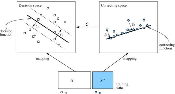
The mappings of inputs x and x∗ in SVM+ are illustrated in Figure 3.1. This figure
shows linear models ψ(x, ω) and ψ∗(x∗, ω∗) in the decision space and correcting space.
However, the mapping Ψ(x) and Ψ∗(x) themselves may be nonlinear, and both the
correcting space are discussed later in Section 3.2.1. It should be noted that the final performance of SVM+ models would depend on the quality of the privileged information.
training ξ
Decision space Correcting space
correcting function decision function X X∗ ξ2 ξ1 mapping mapping ξ2 ξ1 data
Figure 3.1. SVM+ maps the training data simultaneously into the
deci-sion space and the correcting space. Slack variables in the decideci-sion space are represented by the correcting functions in the correcting space.
Mathematically, SVM+ estimates the decision function f(z) = (w,z) +b from the training data (3.1) by solving the following optimization problem:
minimize 1 2kwk 2+γ 2kw ∗k2+C n X i=1 ξi subject to yi((w,zi) +b)≥1−ξi, i= 1, . . . , n, ξi = (w∗,z∗i) +b∗, i= 1, . . . , n, ξ 0, (3.2) with w∈ Rd, b ∈R, w∗ ∈ Rk,b∗ ∈ R, and ξ ∈ Rn + as the variables. In (3.2), C > 0 andγ >0 are two hyperparameters, whereaszandz∗are the feature mappings ofxand x∗. Furthermore, the correcting function ξ
i = (w∗,z∗i) +b∗= (w∗, ψ∗(x∗i)) +b∗ in (3.2)
represents a linear model for the slack. These correcting functions provide additional constraints on the slack variables (errors) in the decision space. The correcting functions are nonnegative because they correspond to slack variables.
The SVM+ replaces the slack variables in standard SVM with a slack function defined in the correcting space. Through the slack function, the additional privileged information is used to model the loss function, which guides the hyperplane learning in the decision space [11]. In contrast, the slack variables in standard SVM are only constrained to nonnegative values, which is often less effective than the slack function in SVM+.
Relative to standard SVM formulation (2.11), this new formulation (3.2) includes: (1) additional termkw∗krestricting the capacity (or VC dimension) of the
correct-ing function;
(2) extra constraints reflecting the influence of the privileged information on train-ing errors.
HyperparametersCandγ control the trade-off between the capacity of decision function (i.e., margin size), the capacity of correcting function, and the number of training errors. Settingγ to zero yields the standard SVM formulation (2.11).
Assuming nonlinear kernels for both decision and correcting spaces, SVM+ has four tuning parameters (two kernel parameters along with C and γ). Model selection with four tuning parameters is quite challenging, and using resampling approaches with finite data often results in very unstable estimated models [4].
Problem (3.2) is commonly solved in its dual form:
maximize n X i=1 αi− 1 2 n X i=1 n X j=1 αiαjyiyj(zi,zj) − 1 2γ n X i=1 n X j=1 (αi+βi−C)(αj+βj −C)(z∗i,z∗j) subject to n X i=1 αiyi= 0, n X i=1 (αi+βi−C) = 0, α0, β0, (3.3)
The solution to SVM+ includes a decision function f(x) = (w,z) + ˆb= (w, ψ(x)) + ˆb = n X i=1 αiyiK(x,xi) + ˆb, (3.4)
and a correcting function
ξ(x∗) = (w∗,z∗) + ˆb∗ = (w∗, ψ∗(x∗)) + ˆb∗ = 1 γ n X i=1 (αi+βi−C)K∗(x∗,x∗i) + ˆb∗, (3.5)
where αi and βi,i= 1, . . . , n, are the solutions of (3.3), and K∗ is a kernel function in
the correcting space. However, only (3.4), the model estimated in the decision space Z, is used for prediction.
Comparing between the solutions of SVM and SVM+, we observe that the SVM solution in (2.8) depends only on the values of pairwise similarities between training vectors defined by the Gram matrix K of elements K(xi,xj) (which defines similarity
between vectors xi and xj). However, the SVM+ solution in (3.4) and (3.5) uses two
expressions of similarities between training vectors: one (K(xi,xj) for xi and xj) that
comes from spaceX, and another one (K∗(x∗
i,x∗j) forx∗i andx∗j) that comes from space
of privileged informationX∗ [10].
Additionally, one can show that w and w∗ can be expressed in terms of training
samples: w= n X i=1 αiyizi, w∗ = 1 γ n X i=1 (αi+βi−C)z∗i,
based on the Karush-Kuhn-Tucker (KKT) conditions.
3.2.1. Kernels in Correcting Space
In this section, we explore several properties of the correcting function, and argue that a (nonlinear) kernel should be used in the correcting space. The correcting function (in the correcting space) represents a unique way that SVM+ handles the additional
privileged information. That is, the SVM+ approach assumes the decision function (3.4) interact differently with training data according to the privileged information via the correcting function (3.5). In SVM+, the correcting function is a real-valued function with its characteristics:
(1) Since the correcting function models the slack variables (in the decision space), as shown in Figure 3.1, the function values have to be nonnegative, ξ(x∗
i)≥0,
for i= 1, . . . , n. Graphically, training samples in the correcting space have to lie on one side of the corresponding correcting function.
(2) According to the definition of slack variables, ξ(xi) = max(1−yif(xi,w),0),
we know ξ(xi) is strictly greater than zero if the data point xi falls within the
margin, such as data points x1,x2, and x3 in Figure 2.2.
(3) A correcting function has to pass through points with zero slack variables. Those points include the support vectors (such as the shaded circle(s) and square(s) in Figure 2.2) and the separable data points.
x∗ ξ(x∗) a b c x∗ ξ(x∗) a b c
Figure 3.2. An arbitrary linear correcting function would violates ξ(x∗)≥0 atx∗=b(left panel) orx∗ =a (right panel).
Now suppose the privileged information is univariate, i.e., x∗ ∈ R or the
dimen-sionality of the privileged information space X∗ is one. It should be obvious that the
correcting function ξ(x∗) cannot be any linear function in the correcting space. As
of a correcting function. First, a few univariate privileged information would violate ξ(x∗) ≥ 0, for instance, ξ(b) < 0 (left panel) andξ(a) <0 (right panel) in Figure 3.2.
Consequently, not all points (privileged information) lie on one side of ξ(x∗). Second,
this linear function only pass through x∗ =c withξ(c) = 0.
Meanwhile, if we assume that the univariate privileged information is bounded,x∗∈
[a, b], the only linear function satisfies the properties is the one that passes through x∗ =b with negative slope or through x∗ =awith positive slope. Both cases are shown
in Figure3.3. However, linear correcting function with eitherξ(b) = 0 orξ(a) = 0 is not ideal and realistic. They both implicitly allow only one support vector. In summary, linear correcting function is not going to be useful, and it might not even work in most situations. x∗ ξ(x∗) a b x∗ ξ(x∗) a b
Figure 3.3. The only two valid linear correcting functions if x∗ ∈[a, b].
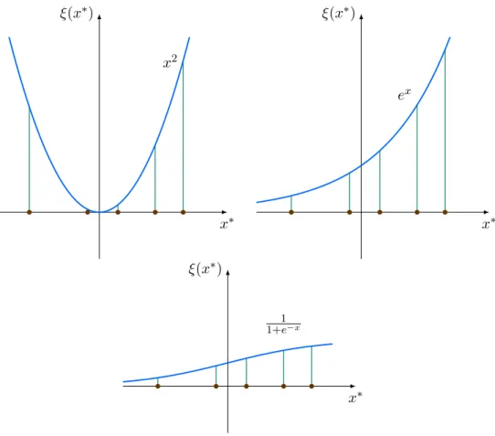
In order to satisfy all three properties of a correcting function, a nonlinear correcting function would be a proper choice. Figure3.4 shows three possible choices of nonlinear correcting functions, namely quadratic, exponential, and sigmoid functions. All three functions have all data points on one side of the function. The quadratic function passes through data points around the vertex withξ(x∗) = 0 or close to zero. The exponential
and sigmoid functions can pass through a wide range of data points. A valid nonlinear correcting function would still need to ensure the kernel matrix K∗ satisfy the Mercer’s
conditions (symmetric and positive semi-definite). In practice, a nonlinear correcting function can be obtained by specifying a nonlinear mapping Ψ∗(x) :x 7→ z∗. Further,
using the “kernel trick” described in Section 2.4, it should suffice to specific a kernel functionK∗(x∗
i,x∗j) for constructing a nonlinear function (hyperplane) in the correcting
space.
To sum up, we use the univariate privileged information and properties of a cor-recting function to argue that a suitable corcor-recting function should be nonlinear, and a kernel should be used in the correcting space. This argument can be extended to high-dimensional privileged information as well.
x∗ ξ(x∗) x2 x∗ ξ(x∗) ex x∗ ξ(x∗) 1 1+e−x
Figure 3.4. Using nonlinear function (quadratic, exponential, sigmoid
3.2.2. Implementation
SVM+ model selection is very difficult due to the fact that the kernelized version of SVM+ binary classifier has four tuning parameters. Hence, the computationally efficient solution of SVM+ optimization becomes critical.
The process of training of standard SVM (or SVM+) involves solving a large Qua-dratic Programming (QP) problem as introduced in Section 2.3 and 3.2. The compu-tational complexity of solving the QP problem (2.12) in SVM training grows as O(n3), where n is the sample size [12]. This is slow when n is large. One of the widely used fast algorithms to train SVM is the Sequential Minimal Optimization (SMO) algorithm proposed by John Platt [13]. This algorithm solves the dual problem of SVM (2.12) in an iterative way. Specifically, SMO breaks a large QP problem into a series of sub-QP problems of the smallest possible size. Each sub-QP problem has only two variables and the analytical solution can be found for this small QP problem, which makes the training much faster. The decision about which pair of variables should be optimized at the current iteration is done by rules of working set selection [13, 14]. This approach was implemented in the LIBSVM package [15] for standard SVM and made this package popular in the machine learning community.
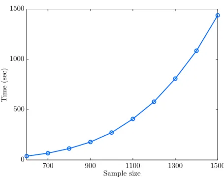
Our initial implementations of SVM+ used a general-purpose convex optimization package CVX [16]. However, the scalability is an issue of using CVX as the solver of the QP problem (3.3). Figure 3.5shows the empirical estimates of computational time for SVM+ implemented in CVX, as a function of training sample size. Clearly, it takes more than 4 minutes to find a solution for the QP problem (3.3) when the training size exceeds 1000 samples. Thus, current model selection strategies become impractical and infeasible, especially the one using exhaustive grid search. Notably, most recent academic papers seem to use general-purpose optimization for their LUPI implementations, as they have shown empirical comparisons only for small training sets (about 200 to 400 samples), and they did not address/describe the challenging issues of model selection. A typical quote from [17]: “On the data set of this size (a few thousand) we found it infeasible to run experiments using SVM+.”
T im e (s ec ) Sample size 700 900 1100 1300 1500 0 500 1000 1500
Figure 3.5. Empirical estimate of computational time of SVM+
imple-mented in CVX as a function of training sample size.
Alternatively, we chose to implement SVM+ using the quadprog package in Matlab Optimization Toolbox. The quadprog package was designed specifically for solving the QP problems, rather than general convex optimization problems. Our implementation involves the selection of the optimization option and also the stopping criterion (tol-erance) optimally tuned for the SVM+ algorithm. Our experiments suggest that the quadprog implementation of SVM+ is capable of handling training data sets of size 1K-5K samples. That is, solving SVM+ optimization problem (for 1K-1K-5K training samples) takes 2-12 seconds on a typical PC.
Next, we describe details of transforming SVM+ dual problem (3.3) into the canonical QP form forquadprog. The objective function of (3.3), reproduced below,
− n X i=1 αi+ 1 2 n X i=1 n X j=1 αiαjyiyj(zi,zj) + 1 2γ n X i=1 n X j=1 (αi+βi−C)(αj+βj −C)(z∗i,z∗j)
can be translated into the following, 1 2 α1 .. . αn α1+β1−C .. . αn+βn−C T H1 H2 α1 .. . αn α1+β1−C .. . αn+βn−C + −1 .. . −1 0 .. . 0 T α1 .. . αn α1+β1−C .. . αn+βn−C , (3.6) where H1= y1y1(z1,z1) · · · y1yn(z1,zn) .. . . .. ... yny1(zn,z1) · · · ynyn(zn,zn) , H2= 1 γ (z∗ 1,z∗1) · · · (z∗1,z∗n) .. . . .. ... (z∗ n,z∗1) · · · (z∗n,z∗n) .
The equality constraints in (3.3),P
αiyi = 0 andP(αi+βi−C) = 0, can be combined
into the matrix form below,
y1 · · · yn 0 · · · 0 0 · · · 0 1 · · · 1 0 · · · 0 α1 .. . αn α1+β1−C .. . αn+βn−C = 0 0 . (3.7)
Further, the inequality constraintsα0 andβ0 in (3.3) are equivalent to 1 −1 . .. . .. 1 −1 α1 .. . αn α1+β1−C .. . αn+βn−C C .. . C , (3.8) and 0 .. . 0 −∞ .. . −∞ α1 .. . αn α1+β1−C .. . αn+βn−C ∞ .. . ∞ ∞ .. . ∞ . (3.9)
Finally, problem (3.3) can be rewritten in a concise QP form,
minimize 1 2x THx+fTx subject to Aeqx=beq, Axb, LB xUB. (3.10)
The objective function 1 2x
THx+fTx is given in (3.6) withx,H, and f defined as
x= α1 .. . αn α1+β1−C .. . αn+βn−C , H = H1 H2 , f = −1 .. . −1 0 .. . 0 ,
respectively. The equality constraintAeqx=beq is described in (3.7) with
Aeq = y1 · · · yn 0 · · · 0 0 · · · 0 1 · · · 1 0 · · · 0 , beq = 0 0 .
The inequality constraints Axb and LBxUB are given in (3.8) and (3.9) with
A= 1 −1 . .. . .. 1 −1 , b= C .. . C , LB= 0 .. . 0 −∞ .. . −∞ , UB= ∞ .. . ∞ ∞ .. . ∞ .
Although SVM+ can be transformed into a canonical QP form (3.10) and solved using any efficient QP solver, it is still not an ideal approach. One reason is that the number of dual variables (Lagrange multipliers) are doubled. Instead of solving ndual
variables in (2.12), we need to solve 2n dual variables in (3.3) or (3.10). This could be an issue when the training sample size is significantly large.
While SVM+ can also be solved by an SMO-style algorithm [18,19], the working set selection method is complicated, and the algorithm is also slow in practice. Moreover, it is unclear how to apply it to linear SVM+ without calculating the kernel matrix, which is becoming more crucial, due to rapidly increasing data in real-world applications [11]. Li et al. proposed two fast algorithms for solving linear and kernel SVM+ in [11]. We summarize both algorithms and comment on their applicabilities below.
(1) Solution for linear SVM+
By absorbing the bias terms into the weight vectors in both decision and correcting spaces, the optimization problem (3.2) (or its dual form (3.3)) can be rewritten as a special form of linear SVM introduced in [20]. Such linear SVM can be solved by using a dual coordinate descent method, and this approach has been implemented in the software package LIBLINEAR [21] which specializes in large linear classification problems. Conveniently, the LIBLINEAR package can be used for solving the linear SVM+ as well. Although using LIBLINEAR to solve the linear SVM+ can significantly enhance the scalability, a nonlinear mapping cannot be used in the correcting space. Utilizing the linear mapping in the correcting space could potentially diminish the advantages of SVM+ based on our arguments in Section 3.2.1.
(2) Solution for kernel SVM+
Instead of solving (3.2), Li et al. considered the l2 loss SVM+ formulation
minimize 1 2kwk 2+γ 2kw ∗k2+C n X i=1 ξi2 subject to yi((w,zi) +b)≥1−ξi, i= 1, . . . , n, ξi = (w∗,z∗i) +b∗, i= 1, . . . , n, ξ 0, (3.11)
by employing thesquared hinge loss. Problem (3.11) is almost identical to (3.2), except theξi2 term in the objective function. Then (3.11) can be rewritten into thel2 lossρ-SVM+ formulation based on thel2 lossρ-SVM introduced in [22]. The dual form of l2 loss ρ-SVM+ shares a similar form with one-class SVM implemented in the software package LIBSVM [15]. Therefore, the LIBSVM package (with one-class option) can be readily used for solving the l2 loss ρ -SVM+ (or equivalently l2 loss SVM+).
The benefits of this strategy are twofold. First, both linear and nonlinear mappings can be applied to the decision and correcting spaces, in contrast to the limitation in linear SVM+. Second, since the SMO algorithm is the core implementation of LIBSVM, this strategy effectively takes advantage of SMO’s efficiency for solving l2 loss SVM+ (either linear or kernel). This strategy is likely to be faster than the SVM+ solver [19] in practice.
3.3. Loss-Order SVM
In this section, we introduce another LUPI-based formulation which utilizes univari-ate privileged information (i.e., the dimensionality of privileged information spaceX∗ is
one orx∗ ∈R).
This univariate information can be an order oracle [2, 23], which gives ordering of the training examples. For example, the posterior probability P(y | x) defines a total ordering. Utilizing the ordering information via a special type of privileged information can result in improved generalization. For survival data described later in Chapter4, the survival time information can be naturally considered as a good indicator for ordering.
Suppose the privileged information is related to (unknown) posterior probability P(y|x), for instance, P(y|x) =g(x∗), (3.12) or x∗=g−1 P(y|x) , (3.13)
whereg is any nonnegative and nondecreasing function. That is, the actual probability values are not important, as long as their correct orderings are preserved. Conceptually,
the privileged information x∗, org(x∗), can be viewed as aconfidence measure, and the
ordering of x∗-values can improve learning (generalization). Further, we consider the
ordering provided by privileged information separately for each class, i.e.,
P(y = +1|x) =g+(x∗) (3.14)
for positive class, and
P(y =−1|x) =g−(x∗) (3.15)
for negative class.
The Loss-Order SVM (LO-SVM) has been proposed as a new formulation under LUPI setting utilizing univariate privileged information [2, 23]. Mathematically, the LO-SVM algorithm solves the optimization problem below:
minimize 1 2kwk 2+C 1 n X i=1 ξi+C2 n X i=1 ζi subject to ξ0, M(ξ+ζ)0, yi((w,xi) +b)≥1−(ξi+ζi), i= 1, . . . , n, (3.16)
with w ∈ Rd, b ∈ R, ξ ∈ Rn+, and ζ ∈ Rn+ as the variables. Here, M is an order-enforcing matrix that requires ξi+ζi ≤ ξj+ζj if g(x∗i) > g(x∗j) for nonzero ξi and ξj.
If C2 ≫ C1, then ζi = 0 for all i, and (3.16) is reduced to standard SVM (2.11). In
practice, the tuning parameters C1 and C2 should be set so that C1 < C2. Otherwise, the solution of (3.16) is dominated by the ordering term.
The corresponding dual form of (3.16) is maximize n X i=1 αi− 1 2 n X i=1 n X j=1 αiαjyiyj(xi,xj) subject to n X i=1 αiyi = 0, n X i=1 (αi+βi−yiκi−yiλi−C1) = 0, n X i=1 (αi+µi−C2) = 0, α0, β0, κ0, λ0, µ0, (3.17) or, equivalently, maximize n X i=1 αi− 1 2 n X i=1 n X j=1 αiαjyiyj(xi,xj) subject to n X i=1 αiyi= 0, n X i=1 (αi−yiκi−yiλi−C1)≤0, n X i=1 (αi−C2)≤0, α0, κ0, λ0, (3.18)
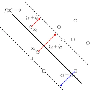
This formulation tries to maintain correct orderings for nonseparable samples from the same class (e.g., training samples with nonzero slack variables) using the privileged information as a confidence measure. Hence, g(x∗
i)> g(x∗j) implies that we have higher
confidence in the class label for training inputxi. For SVM classification, the confidence
ordering provided by the privileged information g(x∗
i) > g(x∗j) is shown in Figure 3.6.
That is, training sample xi should be closer to the margin border (or further away
from the decision boundary), when compared withxj. Thenζi and ζj are the amounts
of “movement” we need for enabling the ordering between xi and xj, as illustrated in
Figure 3.6. f(x) = 0 ξ2+ζ2 ξ1+ζ1 ξ3+ζ3 x1 x2 Figure 3.6. Given g(x∗
1) > g(x∗2), the ζ1 and ζ2 enforce the ordering
ξ1 +ζ1 < ξ2 +ζ2. The ordering should assure that x1 is closer to the margin border, compared withx2.
The LO-SVM algorithm also involves the specification of a nondecreasing function g to ensure g(x∗
i) > g(x∗j) if x∗i > x∗j. In fact, the analytic form of g does not matter,
as long as the ordering holds. In our implementation of LO-SVM, we use the identity function forg.
3.4. SVM+ versus Loss-Order SVM
Although both SVM+ and LO-SVM learning approaches incorporate the privileged information, there are several differences between them. We highlight those differences in this section.
The SVM+ uses the privileged information for modeling (or shaping) the slack vari-ables directly, expecting an improvement in the hyperplane’s separability and leading to better generalization. On the other hand, the LO-SVM considers the privileged informa-tion as a confidence measure (through an appropriate transformainforma-tiong), which provides proper ordering for training samples.
The LO-SVM can be considered as a special case of SVM+ in two aspects:
(1) the privileged information is utilized in an one-dimensional correcting space; (2) the correcting function is a nonlinear one composing with a series of inequalities
which ensures the ordering of samples.
The SVM+ potentially has wider range of applications since there is no limitation in the dimensionality of the privileged information. Still, LO-SVM can be useful for training data with univariate privileged information. The domain of applications and perfor-mances for SVM+ and LO-SVM are discussed later in Chapter 4.
In terms of the computational implementation, the dual form of SVM+ (3.3) contains 2n Lagrange multipliers. In contrast, the dual problem of the LO-SVM (3.18) requires finding 3nLagrange multipliers. Solving (3.18) can become difficult for largen, especially during the process of ordering.
Note that both SVM+ and LO-SVM formulations (3.2) and (3.16) are presented only for linear parameterization; they can be readily extended to nonlinear case using kernels [2].
3.5. Summary
The situation with existence of privileged information is very common. In fact, for almost all machine learning problems there exists some sort of privileged information especially in the era of Big Data. This information cannot be utilized by most standard supervised learning methods developed in statistics and machine learning. Nonetheless,
effectively utilizing this privileged information during training usually results in improved generalization [2].
LUPI is a learning paradigm and a general methodology for utilizing privileged infor-mation about training data. The SVM+ and LO-SVM are two formulations under the LUPI framework. Technically, the SVM+ approach utilizes the privileged information into modeling the training errors (or slack variables) via the correcting function, im-posing additional constraints on slack variables. The LO-SVM considers the privileged information as a confidence measure (through an appropriate transformation g), which provides proper ordering for training samples.
Modeling of Survival Data
Privileged information often appears in modern complex clinical datasets. It could be a patient’s survival time or a patient’s medical history after diagnosis or medical procedure. The most common type of data that include the privileged information is the survival data. In this chapter, we demonstrate the modeling of survival data using LUPI-based learning methods.
4.1. Introduction
A significant proportion of the medical data is a collection of time-to-event observa-tions. Classical examples are the time from birth to cancer diagnosis, from disease onset to death, and from patient’s entry to a study to relapse. All these times are generally known as the survival time, even when the endpoint is something different from death. Methods for survival analysis developed in classical statistics have been used to model such data. Survival analysis focuses on the time elapsed from an initiating event to an event, or endpoint, of interest [24,25]. The models of classical survival analysis describe the occurrence of events by means of survival curves and hazard rates, and analyze their dependence on covariates by means of regression [24]. One classical approach for sur-vival curve estimation is the Cox regression based on the proportional hazards model assumption.
This modeling approach is generally known as the probabilistic (or descriptive) mod-eling. The probabilistic modeling assumes that
(1) the training and future data (x, y) are sampled independently from the same distribution P(x, y);
(2) the distributionP(x, y) is unknown but can be accurately estimated from data.
Classical statistics further makes specific assumptions about the parametric form of a distribution, and uses the training data to estimate its parameters. Clearly, the proba-bilistic approach may produce a poor predictive model if the parametric model is specified incorrectly or if the number of training samples is too small.
On the other hand, machine learning methods focus on estimating (learning) a good predictive model from available data. Specifically, this predictive modeling approach first specifies a wide set of admissible modelsf(x, ω) indexed by abstract set of parametersω, and then estimates the best predictive model from the training data. Further, predictive modeling requires proper specification of the problem setting (formalization) including the loss function used for measuring the quality of prediction, and specification of training and test data [3].
Learning is the process of estimating an unknown dependency between system’s inputs and its output, based on a limited number of observations. When the observations are the survival data, the learning task becomes challenging. The main reason is that there are three types of information in survival data. The first type of information is the input variables, corresponding to ordinary inputs for most machine learning algorithms. Additionally, the survival time and the censoring are two other types of information included in survival data.
The survival time is the duration from the beginning of a study to the occurrence of an event. However, the survival time could be censored and it normally happens when an event is not observed at the end of a study. In such case, the observed survival time is only a lower bound of the true survival time. Both the survival time and censoring information are different from the ordinary input variables as they are only available in the training data.
Therefore, machine learning techniques have not been widely used for survival anal-ysis for two main reasons [26]:
(1) First, the survival time is not necessarily observed in all samples. For instance, subjects might not experience the occurrence of event (death or relapse) during a study, or they dropped out before the end of study. In either case, the survival time is incomplete and only known “up-to-a-point.” This is termed censoring
in biostatistics, which is different from the notion of “missing data” in machine learning.
(2) The second reason is methodological. Machine learning techniques are usually developed and applied under predictive setting, where the main goal is good prediction accuracy for future (or test) samples. In contrast, classical methods in statistics aim at estimating the true probabilistic model underlying available data. So the prediction accuracy is just one of several performance indices. The methodological assumption is that if an estimated model is “correct,” then it should yield good predictions. Therefore, statistical methods often do not clearly differentiate between training (model estimation) and prediction (test) stages.
Several recent studies formalize the problem of survival analysis under the regression setting. For example, the Support Vector Machine (SVM) regression is used to estimate a predictive model for survival time [27, 28, 29]. However, the formalization using regression setting is intrinsically more difficult than classification [4].
Our approach for modeling survival data uses classification setting [26]. We also propose to incorporate the survival time and censoring information into learning by considering them as the privileged information. Learning Using Privileged Information (LUPI) is an advanced learning paradigm, where privileged information about training examples is provided during training stage [2]. This chapter investigates two LUPI-based formulations, SVM+ and LO-SVM, for modeling survival data. The SVM+ formulation considers both the survival time and censoring information. The LO-SVM formulation utilizes only the survival time information.
The chapter is organized as follows. Section 4.2 introduces necessary background on survival data and survival analysis. Section 4.3 defines the formalization for a sur-vival prediction problem. Section 4.4 describes the proposed LUPI-based methods for modeling the survival data. The empirical comparisons for several synthetic and real-life datasets are presented in Section 4.5. Finally, a summary is included in Section4.6.
![Figure 3.3. The only two valid linear correcting functions if x ∗ ∈ [a, b].](https://thumb-us.123doks.com/thumbv2/123dok_us/9911330.2484318/33.918.196.749.488.770/figure-valid-linear-correcting-functions-x-b.webp)