Nonlinear Time Series Analysis in
Financial Applications
RongHui Miao
A thesis submitted for the degree of Doctor of Philosophy
Department of Economics
University of Bath
March 2012
COPYRIGHT
Attention is drawn to the fact that copyright of this thesis rests with its author. A copy of this thesis has been supplied on condition that anyone who consults it is understood to recognise that its copyright rests with the author and they must not copy it or use material from it except
as permitted by law or with the consent of the author.
This thesis may be made available for consultation within the University Library and may be photocopied or lent to other libraries for the purposes of consultation.
Page | 1
Acknowledgements
I would like to take this opportunity to express my gratitude to the people who had been helpful and supportive during my study.
First and foremost, I am enormously grateful to my supervisor, Professor Christos Ioannidis, for his patient guidance, invaluable suggestions, and continuous encouragement. Without him, this thesis would not have been possible, and his feedback contributed greatly to this thesis. I thank him also for his faith in my research ability during these years. I remember our many stimulating and constructive discussions about interesting research topics in finance and other subjects. I have also learnt from him his rigorous approach to academic research.
I am also grateful to Dr Julian Williams, who is now a Lecturer in Finance at the University of Aberdeen Business School. I have learnt from Julian that innovative ideas and critical thinking are essential for becoming a good researcher. I enjoyed very much when I was working with Julian and Christos on a chapter about interest rate models that has been published in "Optimization and Its Applications, in Handbook of Financial Engineering, Series: Springer Optimization and Its Applications Vol. 18, 2008 ".
I would also like to thank Dr Giovanni Calice, who is now a Lecturer in Finance at the University of Southampton Management School, for providing the data that are used in the last chapter of this thesis. I enjoyed working with Giovanni and Christos on our paper based on this chapter. Furthermore, Giovanni was always available for discussing interesting research topics. His research enthusiasm about the effect of credit risks on financial market's stability has also inspired me a lot in this research area.
I would like to thank my fellow doctoral students for their constructive discussions on various issues in research. Special thanks go to Xinyang Li, my former fellow at the School of Management, for her helpful advice, both academically and personally.
Last, but never least, I thank my parents for patience and precious support during my study.
Page | 2
Contribution of Authors
The last chapter of this thesis is a collaboration between Rong Hui Miao, Christos Ioannidis and Giovanni Calice. Christos Ioannidis is a Professor of Finance and Economics at the Department of Economics, University of Bath. Giovanni Calice is a PhD student at the Department of Economics, University of Bath and also a Lecturer in Finance at the School of Management, University of Southampton. Rong Hui Miao performed the data analysis, econometric modelling and empirical results that make up the chapter. Rong Hui Miao, Professor Christos Ioannidis and Dr. Giovanni Calice jointly developed the main research ideas. Rong Hui Miao and Professor Christos Ioannidis discussed revisions of the chapter. Professor Christos Ioannidis has contributed to the empirical results and conclusion sections of this chapter (about 20% in writing). Dr. Giovanni Calice supplied the data and contributed to the literature review of this chapter (about 10% in writing).
Page | 3
Abstract
The purpose of this thesis is to examine the nonlinear relationships between financial (and economic) variables within the field of financial econometrics. The thesis comprises two reviews of literatures, one on nonlinear time series models and the other one on term structure of interest rates, and four empirical essays on financial applications using nonlinear modelling techniques.
The first empirical essay compares different model specifications of a Markov switching CIR model on the term structure of UK interest rates. We find the least restricted model provides the best in-sample estimation results. Although models with restrictive specifications may provide slightly better out-of-sample forecasts in directional movements of the yields, the economic gains seem to be small.
In the second essay, we jointly model the nominal and real term structure of the UK interest rates using a three-factor essentially affine no-arbitrage term structure model. The model-implied expected inflation rates are then used in the subsequent analysis on its nonlinear relationship with the FTSE 100 index return premiums, utilizing a smooth transition vector autoregressive model. We find the model implied expected inflation rates remain below the actual inflation rates after the independence of the Bank of England in 1997, and the recent sharp decline of the expected inflation rates may lend support to the standing ground of the central bank for keeping interest rates low. The nonlinearity test on the relationship between the FTSE 100 index return premiums and the expected inflation rates shows that there exists a nonlinear adjustment on the impact from lagged expected inflation rates to current return premiums.
The third essay provides us additional insight into the nature of the aggregate stock market volatilities and its relationship to the expected returns, in a Markov switching model framework, using centuries-long aggregate stock market data from six countries (Australia, Canada, Sweden, Switzerland, UK and US). We find that the Markov switching model assuming both regime dependent mean and volatility with a 3-regime specification is capable to captures the extreme movements of the stock market which are short-lived. The volatility feedback effect that we studied on each of these six countries shows a positive sign on anticipating a high volatility regime of the
Page | 4
current trading month. The investigation on the coherence in regimes over time for the six countries shows different results for different pairs of countries.
In the last essay, we decompose the term premium of the North American CDX investment grade index into a permanent and a stationary component using a Markov switching unobserved component model. We explain the evolution of the two components in relating them to monetary policy and stock market variables. We establish that the inversion of the CDX index term premium is induced by sudden changes in the unobserved stationary component, which represents the evolution of the fundamentals underpinning the risk neutral probability of default in the economy. We find strong evidence that the unprecedented monetary policy response from the Fed during the crisis period was effective in reducing market uncertainty and helped to steepen the term structure of the CDX index, thereby mitigating systemic risk concerns. The impact of stock market volatility on flattening the term premium was substantially more robust in the crisis period. We also show that equity returns make a significant contribution to the CDX term premium over the entire sample period.
Page | 5
Table of Contents
Chapter I Introduction ... 15
Chapter II A review of nonlinear regime switching models ... 19
II.1 Threshold Models ...20
II.1.1 Basic STR Model ...20
II.1.2 Inference in STR models ...22
II.1.2.1 Test Linearity against STR ...22
II.1.2.2 Specification of STR models ...23
II.1.2.3 Estimation of STR models ...24
II.1.2.4 Model adequacy tests of STR models ...24
II.2 Markov-switching Models ...24
II.2.1 Basic model ...24
II.2.2 Estimating a basic Markov-switching model using Hamilton filter ...26
II.2.3 2.2.5 Specification test of Markov-switching models ...28
Bibliography ... 29
Chapter III A review of the models in the term structure of interest rates ... 32
III.1 Information contained in the term structure of interest rates ...32
III.2 Definitions of term premia ...33
III.3 Regression analysis of term premia ...35
III.3.1 Testing on forward term premia ...35
III.3.2 Testing on long-term premia ...37
III.3.3 The Campbell-Shiller (1991) puzzle ...37
III.3.4 Fama-Bliss (1987) and Cochrane-Piazzesi (2005) regression analysis ...40
III.4 Factor models in estimating term structure of interest rates ...50
III.4.1 Principal components ...53
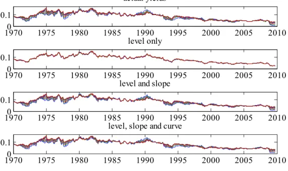
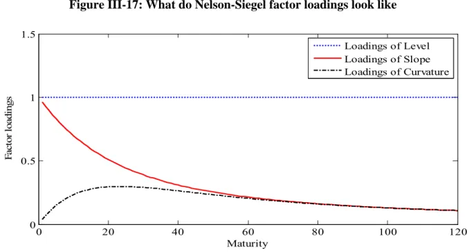
III.4.2 Nelson-Siegel factor model ...57
III.4.2.1 Estimation of the dynamic Nelson-Siegel factor model using Kalman filter ...58
Page | 6
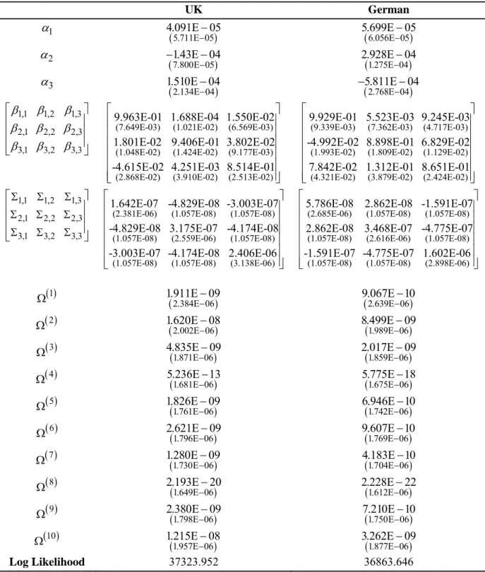
III.4.2.2 Estimation results ...62
III.5 No-arbitrage factor models ...67
III.5.1 No-arbitrage conditions and the stochastic discount factor in term structure model ...68
III.5.2 Short rate model ...72
III.5.3 Multi-factor affine model ...74
III.5.3.1 Discussion on the specification of market price of risk in affine term structure models ...77
Bibliography ... 78
Appendix III ... 81
Chapter IV A Markov switching extension of the short rate model ... 88
IV.1 Introduction ...88
IV.2 Single regime CIR model ...89
IV.3 Markov switching CIR model ...91
IV.3.1 Maximum Likelihood Estimation of Markov switching CIR model ...92
IV.4 Empirical results ...94
IV.5 Ex-ante pricing performance of the models ...103
IV.6 Conclusion ...105
Bibliography ... 106
Appendix IV ... 108
Chapter V Joint Modelling of the Nominal and Real Term Structure of Interest Rates and the relation between expected inflation rates and stock return risk premium ... 114
V.1 Motivation and Literature Review ...115
V.1.1 Empirical behaviour of nominal term premia in no-arbitrage factor models120 V.1.2 Empirical estimates of inflation risk premia ...120
V.2 Inflation index-linked gilts ...123
V.3 Essentially affine term structure of nominal and real interest rates ...125
V.3.1 State equation ...125
Page | 7
V.3.3 Nominal bond pricing ...127
V.3.4 Real bond pricing ...128
V.3.5 Nominal and real term premia ...129
V.3.6 Inflation risk premia and expected inflation ...131
V.4 Data ...131
V.5 Principal component analysis and simple regressions ...141
V.6 Estimation ...145
V.7 Empirical results ...147
V.8 The relation between stock returns and expected inflation ...160
V.8.1 The STVAR model ...162
V.8.2 Specification tests for the STVAR models ...164
V.8.2.1 Linearity test ...164
V.8.2.2 Model adequacy tests ...166
V.8.2.2.1 Test of serially correlated errors ...166
V.8.2.2.2 Tests for parameter constancy ...167
V.8.2.2.3 Test for no remaining nonlinearity ...168
V.8.3 Empirical result ...168
V.9 Conclusion ...174
Bibliography ... 175
Appendix V ... 180
Chapter VI The stock market risk return Trade-off: evidence from six countries using centuries-long data ... 189
VI.1 Introduction ...189
VI.2 Literature review ...190
VI.3 Econometric models ...193
VI.3.1 Single regime mean and variance (Model 1) ...193
VI.3.2 Single regime mean and multi-regime variance (Model 2) ...194
VI.3.3 Multi-regime mean and variance (Model 3) ...195
Page | 8
VI.3.5 Multi-regime mean, variance and autoregressive coefficient with learning
(Model 5) ...196
VI.4 Data ...198
VI.5 Estimation Results ...203
VI.5.1 Australia ...206 VI.5.2 Canada ...213 VI.5.3 Sweden ...218 VI.5.4 Switzerland ...223 VI.5.5 UK ...228 VI.5.6 US ...232
VI.5.7 Volatility feedback effect ...236
VI.5.8 The co-movements (integration) of the stock markets ...238
VI.6 Conclusion ...241
Bibliography ... 242
Appendix VI ... 245
Chapter VII A Markov Switching Unobserved Component Analysis of the CDX Index Term Premium ... 250
VII.1 Introduction ...250
VII.2 Motivation and Methodology...255
VII.2.1 Stationary and Random Walk Components in State Space Representation ...259
VII.2.2 State Space Model with Markov Switching Disturbances ...262
VII.2.3 Estimation procedure ...264
VII.3 Data ...268
VII.4 Empirical Results ...271
VII.4.1 Model selection tests ...272
VII.4.2 Estimates of the Markov-switching unobserved component model ...275
VII.4.3 VAR Analysis ...279
Page | 9
Bibliography ... 286 Appendix VII ... 289 Chapter VIII Summary and conclusion ... 304
Page | 10
List of Tables
Table III-1: UK and German Nelson-Siegel model estimates and standard errors ...63
Table III-2: Descriptive statistics ...81
Table III-3: Fama-Bliss regression and "complementary regression" results ...82
Table III-4: Time series and cross sectional regressions of 1-year excess bond returns on all forward rates ...83
Table III-5: Time series and cross sectional regressions of 2-year excess bond returns on all forward rates ...84
Table IV-1: Estimated models ...94
Table IV-2: Descriptive statistics ...95
Table IV-3: Parameter estimates of various models ...96
Table IV-4: Likelihood ratio tests ...100
Table IV-5: MSE and FDT statistics ...104
Table IV-6: Pesaran-Timmermann test ...105
Table V-1: Descriptive statistics of nominal zero-coupon bond yields ...136
Table V-2: Descriptive statistics of real zero-coupon bond yields ...137
Table V-3: Principal component analysis ...143
Table V-4: Parameter estimation results ...148
Table V-5: Projection of the break-even rates on nominal yields within different sample periods ...159
Table V-6: Linear approximation of LSTVAR and ESTVAR models ...165
Table V-7: Nested model selection hypothesis tests ...165
Table V-8: Descriptive statistics of r and ...169
Table V-9: Results for linearity test and model selection test ...170
Table V-10: Maximum likelihood estimates of the LSTVAR models ...171
Table V-11: Model adequacy tests ...173
Table V-12: Review of recent estimations of inflation risk premia and inflation expectation ...180
Table VI-1: Data sources and time span of the stock return data ...199
Table VI-2: Descriptive statistics of the stock market return series for each country ...199
Table VI-3: Model specification test using Hansen 1992 test procedure ...205
Table VI-4: Estimation results (Australia) ...206
Table VI-5: Ljung-Box Q statistics for autocorrelation effect and Q2 statistics for ARCH effect on the residuals (Australia) ...207
Table VI-6: Correlation between smoothed probability of high (low and high) volatility regime across 2-regime (3-regime) models - Australia ...209
Table VI-7: Estimation result (Canada) ...214
Table VI-8: Ljung-Box Q statistics for autocorrelation effect and Q2 statistics for ARCH effect on the residuals (Canada) ...215
Table VI-9: Correlation between smoothed probability of high (low and high) volatility regime across 2-regime (3-regime) models - Canada ...215
Table VI-10: Estimation result (Sweden) ...218
Table VI-11: Ljung-Box Q statistics for autocorrelation effect and Q2 statistics for ARCH effect in the residuals (Sweden) ...220
Table VI-12: Correlation between smoothed probability of high (low and high) volatility regime across 2-regime (3-regime) models - Sweden ...221
Page | 11
Table VI-13: Estimation result (Switzerland) ...223
Table VI-14: Ljung-Box Q statistics for autocorrelation effect and Q2 statistics for ARCH effect in the residuals (Switzerland) ...224
Table VI-15: Correlation between smoothed probability of high (low and high) volatility regime across 2-regime (3-regime) models - Switzerland ...225
Table VI-16: Estimation result (UK) ...228
Table VI-17: Ljung-Box Q statistics for autocorrelation effect and Q2 statistics for ARCH effect on the residuals (UK) ...229
Table VI-18: Correlation between smoothed probability of high (low and high) volatility regime across 2-regime (3-regime) models - UK ...230
Table VI-19: Estimation result (US) ...232
Table VI-20: Ljung-Box Q statistics for autocorrelation effect and Q2 statistics for ARCH effect on the residuals (US) ...233
Table VI-21: Correlation between smoothed probability of high (low and high) volatility regime across 2-regime (3-regime) models - US ...235
Table VI-22: Coherence in regimes between pairs of countries ...239
Table VI-23: Estimation results of Model 5 for each country ...245
Table VII-1: Mean and standard deviation of the CDX 5-year (CDX5Y), CDX 10-year (CDX10Y) and Term Premium (TP) for different sample periods ...258
Table VII-2: Descriptive statistics of the data series ...270
Table VII-3: Model selection results ...273
Table VII-4: Likelihood ratio tests on constraint 12 21 0 ...274
Table VII-5: Likelihood ratio tests within groups ...274
Table VII-6: Residual diagnostic tests...274
Table VII-7: Estimation results of Model 8 ...276
Table VII-8: Generalized variance decomposition of DIFRW and STAT in the pre-financial crisis period(September 13, 2004 to January 03, 2008) ...282
Table VII-9: Generalized variance decomposition of DIFRW and STAT in the post-financial crisis period (January 04, 2008 to July 23, 2009) ...283
Page | 12
List of Figures
Figure III-1: Unrestricted and restricted coefficients ...44
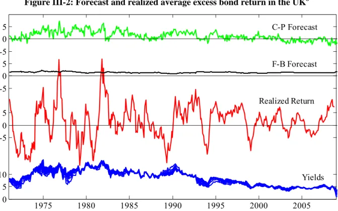
Figure III-2: Forecast and realized average excess bond return in the UK ...45
Figure III-3: Forecast and realized average excess bond return in the US ...45
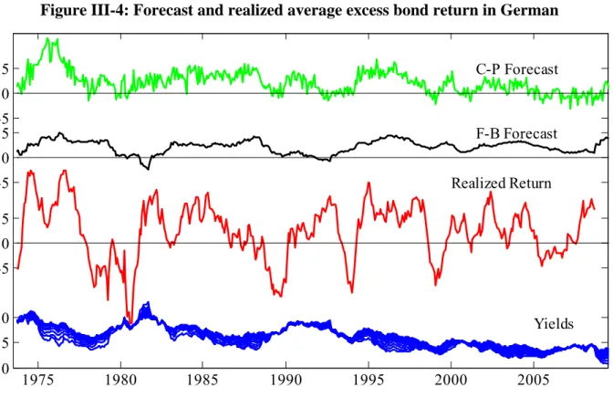
Figure III-4: Forecast and realized average excess bond return in German ...46
Figure III-5: UK 2-year holding period regression coefficients ...48
Figure III-6: US 2-year holding period regression coefficients ...48
Figure III-7: German 2-year holding period regression coefficients ...49
Figure III-8: US 1 to 5 years Zero-Coupon-Yield level and slope (06/1952–12/2008) ...51
Figure III-9: UK 1 to 10 years Zero-Coupon-Yield level and slope (01/1970–09/2009) ...51
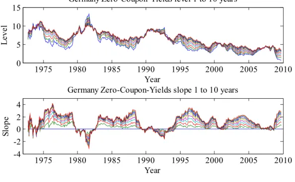
Figure III-10: German 1 to 10 years Zero-Coupon-Yield level and slope (09/1972–09/ 2009) ...52
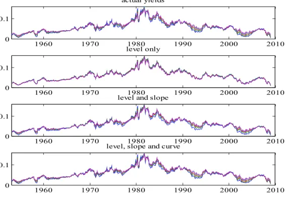
Figure III-11: Replicate the US zero coupon bond yields using principal components ...55
Figure III-12: US replication residuals square ...55
Figure III-13: Replicate the UK zero coupon bond yields using principal components ...56
Figure III-14: UK replication residuals square ...56
Figure III-15: Replicate the German zero coupon bond yields using principal components ...57
Figure III-16: German replication residuals square ...57
Figure III-17: What do Nelson-Siegel factor loadings look like ...58
Figure III-18: UK Nelson-Siegel factors ...64
Figure III-19: German Nelson-Siegel factors ...65
Figure III-20: Residual square of the fitted UK yields ...65
Figure III-21: Residual square of the fitted German yields ...66
Figure III-22: Observed and fitted UK yields ...66
Figure III-23: Observed and fitted German yields ...67
Figure IV-1: UK zero-coupon bond yields (%, January 1970 to September 2010) ...97
Figure IV-2: Smoothed state probabilities of regime 0 for various models ...98
Figure IV-3: Observed 3-month rates and fitted 3-month rates from models ...99
Figure IV-4: Observed 5-year rates and fitted 5-year rates from models ...99
Figure IV-5: Observed 10-year rates and fitted 10-year rates from models ...100
Figure IV-6: Snap shot of the yields between January 2003 and September 2010 ...101
Figure IV-7: Recursive AIC and BIC ...102
Figure V-1: UK nominal zero-coupon yields for various maturities ...133
Figure V-2: UK RPI(Percentage change over 12 months - all items) ...134
Figure V-3: UK zero-coupon real yields for various maturities ...135
Figure V-4: UK average nominal yield curve with +/- 2 S.E. bounds ...138
Figure V-5: UK nominal yield volatility curve with +/- 2 S.E. bounds ...138
Figure V-6: UK average real yield curve with +/- 2 S.E. bounds ...139
Figure V-7: UK real yield volatility curve with +/- 2 S.E. bounds ...139
Figure V-8: UK nominal yield autocorrelation curve with +/- 2 S.E. bounds ...140
Figure V-9: UK real yield autocorrelation curve with +/- 2 S.E. bounds ...141
Figure V-10: Factor loadings of nominal yields on principal components ...143
Figure V-11: Factor loadings of real yields on principal components ...144
Figure V-12: Filtered three unobserved factors ...149
Figure V-13: Observed and fitted nominal yields (3-month, 1-year, 3-year and 5-year) ...149
Page | 13
Figure V-15: Observed and fitted real yields (4-year, 5-year, 6-year and 7-year) ...150
Figure V-16: Observed and fitted real yields (8-year, 9-year and 10-year) ...151
Figure V-17: 5-year nominal yields and term premia ...152
Figure V-18: 10-year nominal yields and term premia ...152
Figure V-19: 5-year real yields and term premia ...153
Figure V-20: 10-year real yields and term premia ...153
Figure V-21: 10-year break-even rate and inflation risk premia ...154
Figure V-22: Term structure of the average nominal and real term premia with +/- 2 S.E. bounds ...155
Figure V-23: Term structure of the volatility of nominal and real term premia with +/- 2 S.E. bounds ...155
Figure V-24: Term structure of the autocorrelation of nominal and real term premia with +/- 2 S.E. bounds ...156
Figure V-25: Term structure of the inflation risk premia (average, volatility and autocorrelation curves) with +/- 2 S.E. bounds ...156
Figure V-26: The observed and expected 1 month inflation rates ...157
Figure V-27: Observed and expected annual inflation rates ...158
Figure V-28: 4-year to 10-year expected inflation rate ...159
Figure V-29: Monthly stock return risk premium (FTSE100) and changes of monthly expected inflation rates ...169
Figure V-30: Logistic transition function from LSTVAR model with st t4 ...172
Figure V-31: Logistic transition function from LSTVAR model with st rt5 ...173
Figure VI-1: Australian stock market index and stock return ...200
Figure VI-2: Canadian stock market index and stock return ...200
Figure VI-3: Swedish stock market index and stock return ...201
Figure VI-4: Switzerland stock market index and stock return ...201
Figure VI-5: The UK stock market index and stock return ...202
Figure VI-6: The UK stock market index and stock return (Sep. 1902 to Sep. 2007) ...202
Figure VI-7: The US stock market index and stock return ...203
Figure VI-8: The US stock market index and stock return (Sep. 1902 to Sep. 2007) ...203
Figure VI-9: Australian stock market return series and Model 2-AR(1)'s smoothed posterior probability of observing a high volatility regime (2-regime) ...209
Figure VI-10: Australian stock market return series and Model 2-AR(1)'s smoothed posterior probability of observing a low volatility regime (3-regime) ...210
Figure VI-11: Australian stock market return series and Model 2-AR(1)'s smoothed posterior probability of observing a high volatility regime (3-regime) ...211
Figure VI-12: Australian stock market return series and Model 2-AR(0)'s smoothed posterior probability of observing a high volatility regime (3-regime) ...212
Figure VI-13: Australian stock market return series and Model 3-AR(0)'s smoothed posterior probability of observing a high volatility regime (3-regime) ...213
Figure VI-14: Canadian stock market return series and Model 3-AR(1)'s smoothed posterior probability of observing a high volatility regime (2-regime) ...215
Figure VI-15: Canadian stock market return series and Model 3-AR(1)'s smoothed posterior probability of observing a low volatility regime (3-regime) ...217
Figure VI-16: Canadian stock market return series and Model 3-AR(1)'s smoothed posterior probability of observing a high volatility regime (3-regime) ...218
Page | 14
Figure VI-17: Sweden stock market return series and Model 3-AR(1)'s smoothed posterior probability of observing a low volatility regime (3-regime) ...222 Figure VI-18: Sweden stock market return series and Model 3-AR(1)'s smoothed posterior probability of observing a high volatility regime (3-regime) ...222 Figure VI-19: Switzerland stock market return series and Model 3-AR(1)'s smoothed
posterior probability of observing a high volatility regime (2-regime) ...225 Figure VI-20: Switzerland stock market return series and Model 4-AR(1)'s smoothed
posterior probability of observing a low volatility regime (3-regime) ...227 Figure VI-21: Switzerland stock market return series and Model 4-AR(1)'s smoothed
posterior probability of observing a high volatility regime (3-regime) ...227 Figure VI-22: The UK stock market return series and Model 4-AR(1)'s smoothed posterior probability of observing a low volatility regime (3-regime) ...231 Figure VI-23: The UK stock market return series and Model 4-AR(1)'s smoothed posterior probability of observing a high volatility regime (3-regime) ...232 Figure VI-24: The US stock market return series and Model 2-AR(1)'s smoothed posterior probability of observing a low volatility regime (3-regime) ...235 Figure VI-25: The US stock market return series and Model 2-AR(1)'s smoothed posterior probability of observing a high volatility regime (3-regime) ...236 Figure VI-26: Time evolution of the coherence in regimes between pairs of countries (1) ...240 Figure VI-27: Time evolution of the coherence in regimes between pairs of countries (2) ...241 Figure VI-28: Time evolution of the coherence in regimes between pairs of countries (3) ...241 Figure VII-1: CDX-5 year, CDX-10 Year and CDX term premium ...270 Figure VII-2: Actual plots of: FFR, SLOPE101, SP500RTN and VIX ...271 Figure VII-3: Snapshot of the stationary component in its low volatility regime ...277 Figure VII-4: Stationary component and filtered state probability of its high volatility regime ...289 Figure VII-5: Random walk component and filtered state probability of its high volatility regime ...290 Figure VII-6: Conditional variance of the term premium and filtered state probability of high volatility regime for each component ...291 Figure VII-7: Accumulative generalized impulse response functions of the VAR model in the pre-financial crisis period (September 13, 2004 to January 03, 2008) ...292 Figure VII-8: Accumulative generalized impulse response functions of the VAR model in the post-financial crisis period (January 04, 2008 to July 23, 2009) ...293
Page | 15
Chapter I
Introduction
In recent years a major class of nonlinear time series models - regime switching model - has become a popular workhorse in many economic and financial studies. For example, studies dedicated to business cycles, equity return forecasting, term structure of interest rates and exchange rates volatility modelling, have been adopting increasingly a regime switching approach to describe the time series properties of economic and financial variables. Why the regime switching models are so attractive to researchers? Arising from practical aspects of modelling dynamic economic and financial time series, researches often observe variables undergo either/both permanent structural changes or/and recurrent temporary changes over a long sample period. The most well-known example of this type is the repeatedly appearance of expansion and recession phrases in business cycles. The apparent time inconsistency patterns make researchers believe that the constant parameter time series models may not be able to incorporate the observed regime changes in practice. One way to solve this problem is to build a stochastic process into the time series model that is capable to describe the regime switches in the mean or/and variance of the variables being studied. Although we do not directly observe these regime switches at any point in time, we may draw inferences on the regimes in operation of a known stochastic process, and hence the possible future switches in forecast.
This dissertation comprises a collection of four empirical essays in nonlinear time series analysis of economic/financial variables. Two of them involve the term structure of interest rates modelling. The term structure of interest rates plays a central role in economy, both theoretically and practically. While policy makers conduct monetary policy by shifting interest rates at the short end of yield curve, longer term yields give markets’ reflection of future economic health. When expectations about future rates change, the yield curve reacts as bonds reprice to reflect these expectation changes. Moreover, longer term yields also compound liquidity risk premium and nonlinear convexity premium. Therefore, the movements in longer end of the term structure reflect not only the revision of expectation but also various risk premiums.
Giving the importance of interest rate modelling, the related econometric estimation and forecasting methods have received tremendous attention in recent years. One popular
Page | 16
approach is to incorporate a regime switching feature into the term structure models, which allows the pricing kernel to be regime dependent. Many studies in interest rate modelling have shown empirical evidence of regime switches in short rates. However, none of them (except Driffill, et al.(2009)) considers the impact of different model specifications on the performance of model's forecasting ability. In Chapter IV, we estimate a nonlinear Markov switching CIR model on the term structure of UK interest rates and evaluate different parameterizations of the model in terms of real-time one-step-ahead bond pricing performance. We conduct a series of model specification tests on a battery of models that employ different parameter restrictions on the short rate equation. By doing so, we provide a comprehensive Markov switching CIR model specification analysis on the UK data that varies from January 1970 to September 2010.
The issue of the term structure modelling is further discussed in Chapter V, where we jointly model the nominal and real term structure of UK interest rates. The expected rate of inflation is an important economic variable to both policy makers and investors. On the one hand, it measures the credibility of central bank’s monetary policy aiming at anchoring the long term inflation rate around its target level. On the other hand, the inflation risk premia demanded by investors, if non-negligible, would contaminate the interpretation of the break-even inflation rate as a measure of the credibility widely used. However, due to the unobserved nature of real rates, expected inflation rates and the inflation risk premia, making correct identification of these quantities in reality is difficult. To overcome this difficulty, we decompose the nominal term structure of interest rates into real interest rates, expected inflation rates and inflation risk premia by employing a three-factor essentially affine no-arbitrage term structure model on the UK data. The model implied expected inflation rate is then used in the subsequent nonlinear analysis of the relation between stock return premiums and inflation rates.
In Chapter VI, we investigate the risk-return trade-off in stock market. In this study, we provide additional insight into the nature of the aggregate stock market volatilities and its relations to expected returns, in a Markov switching model using centuries-long aggregate stock market data from six countries (Australia, Canada, Sweden, Switzerland, the United Kingdom and the United States). We consider a wide range of models in this study. By relaxing restrictions on the multi-regime switching parameters in each step, we estimated a series of models either allowing each of the expected mean and volatility of the stock return
Page | 17
to switch or permitting both moments of the stock return to shift regimes over time. In contrast to most studies in Markov switching modelling of stock returns that assuming two regimes, we also consider three-regime specification for the variation of stock returns. This seemingly subtle complication, as compared to the conventional two regimes assumption, allows a richer inter-temporal relation between the expected mean and volatility of the stock return. We also investigate into the "volatility feedback effect" hypothesis that has been documented extensively in literature. We make different assumptions about the information available to market investors. By allowing investors to learn about the current prevailing volatility regime based on different information set prior to the current trading period, we are able to see the effect on the additional risk premium required by investors in anticipating future volatility changes.
In the final chapter, we estimate a Markov switching unobserved component model to explain the evolution of the term premium for the North American CDX index. The term premium of the CDX index, which is measured as the difference between a longer maturity CDX index series and a shorter maturity one (e.g. the difference between the CDX 10-Year index and the CDX 5-Year index), can be viewed as representing the 5-year forward uncertainty regarding corporate default after the next 5 years. Accordingly, the CDX term premium can be interpreted as an early warning market indicator of improvement or deterioration in macroeconomic conditions 5 years hence. Our interest in this study is to study how the factors themselves (not the factor loadings) drive the dynamics of the term premium. To characterize the observed patterns of volatility jumps on the CDX index term premium, we allow on the innovation terms a regime switching process, following two distinct first-order Markov chain variables. We consider an appropriately specified Markov Switching Unobserved Components model as a reliable measure of volatility dynamics of the CDX index spread curve and investigate the presence and significance of both monetary policy adjustments and stock market returns for the US economy over the sample period September 2004 - July2009.
This dissertation is organized as follows. In Chapter II, we give a short review of the nonlinear models used in this dissertation. Chapter III reviews the models of the term structure of interest rates in a linear modelling fashion. Chapter IV presents the study of the Markov switching extension of the short rate model on the UK data. Chapter V discusses the joint modelling of the UK's nominal and real term structure of interest rate with a subsequent
Page | 18
analysis on the relation between stock return premium and the expected inflation rates based on a nonlinear smooth transition vector autoregressive model. Chapter VI investigates the risk-return trade-off in stock market in a flexible Markov switching modelling framework by using century-long aggregate stock market data from six countries. Chapter VII presents the Markov switching unobserved component modelling of the CDX term premium in the US market. Finally, Chapter VIII concludes.
Page | 19
Chapter II
A review of nonlinear regime switching models
Generally speaking, regime switching models can be classified into two groups: threshold regime switching models, and Markov regime switching models. The main difference between the two groups of models is that they adopt different assumptions on the stochastic process of the regime switching variable. Tong (1983) proposed a threshold regime switching model that assumes the regime switching variable is an unobserved threshold, and regimes are defined as above or below the value of the threshold variable. Later, developments in Chan and Tong (1986) and Tong (1990) augmented the threshold variable to be a lagged endogenous variable, which constitutes the so-called threshold autoregressive (TAR) model. By connecting the TAR model with the “smooth transition” idea in Bacon and Watts (1971), researchers devised a general smooth transition regression (STR) model. The empirical appeal of this STR model is that it allows economic variables to transit gradually from one regime to another rather than suddenly change at a fixed threshold value. Maddala (1977) replaced the smoothing function from cumulative distribution function to logistic function, which became a popular choice for the transition function thereafter. With the combination of the STR model and the assumption that the threshold variable is a lagged endogenous variable, Terasvirta (1994) came up with the popularized smooth autoregressive (STAR) model.
Markov regime switching models, which were initially introduced by Goldfeld and Quandt (1973) and popularized by Neftiçi (1982) and Hamilton (1989b), assume that the switching variable follows a Markov chain process. In his empirical study of the U.S. business cycles, Hamilton (1989b) assumes fundamental macroeconomic variables, such as GNP and real output growth, behave differently depending on which state the economy is in at the time. The shifts of states between expansion and contraction of the economy are governed by an unobservable regime switching variable that follows a Markov chain process. The regime switching variable takes two values, 0 and 1, to represent contraction and expansion states of the economy, respectively. Markov regime switching models were firstly invoked in macroeconomic time series studies, particularly in business cycle literatures. Since then, a number of empirical studies have established its statistical advances over the traditional constant parameter time series models. Recent developments in the Markov
Page | 20
regime switching literature on business cycle modelling are surveyed in Hamilton and Raj (2002) and Raj (2002).
II.1 Threshold Models
Early development of the threshold model is based on the discrete threshold transition model. Bacon and Watts (1971) first suggested the phrase “smooth transition”, and showed how the local linear equations can be modelled as a smooth change from one linear extreme to the other when linked to a continuous transition variable. In econometric literature, Goldfeld and Quandt (1973) is the first to propose the following model
1 2 1 2 1 2 1 1 1 1, . 0, t t t t t t t t t t t t t y D z D z D z D z x D z u D z u z c D z z c (II.1)It says when the transition variable zt c , the regression intercept will be 2 , slope parameter will be 2, and the error term will be u2t, otherwise the regression is run on the set of parameters with subscript of 1. In terms of estimation, they suggest a simplified approximation of D z
t , that is a cumulative distribution function with mean c and variance2 , as depicted by (II.2):
2
2 1 1 exp . 2 2 t z t z c D z dz
(II.2)II.1.1 Basic STR Model
The Basic STR model takes the following specification
' ' , ; , 1, 2,..., , t t t t t y x x G c s u t T (II.3)where xt is a vector of explanatory variables consisting of lagged endogenous and exogenous variables, i.e. xt
1,x1t,...,xpt
'
1,yt1,...,yt m ; ,...,z1t ztn
'; and are two different sets of parameters, i.e.
0, ,...,1 p
' and
0, ,...,1 p
'; ut is a sequence of i.i.d. errors; G is a continuous transition function customarily bounded between 0 and 1.Page | 21
Conventionally, G is a function of three elements, among which is a positive identification restriction that indicates the speed of transition from one regime to the other, c is a location parameter that determines where the transition takes place, and st is the transition variable. There are many ways to specify the transition variable st. Terasvirta (1994) defines the STAR model by specifying the transition variable as a lagged endogenous variable, which is st yt d with d 0. Alternatively, the transition variable can be an exogenous variable, like st zt, or a nonlinear function of the lagged endogenous variable,
like
';
t t
s h x with xt'
yt1,...,yt m
for some nonlinear function h conditioned on the parameter vector . Furthermore, the transition variable can be a function of time trend, i.e.t
s t, as in Lin and Terasvirta (1994) that allows smooth time varying parameters.
From (II.3) we see the STR model nests two linear equations, which represent the two local regimes: '
t t t
y xu when G0, and yt xt'
ut when G1. If 0 G 1, the model describes the continuum of states in between the two local regimes. A practical issue about the STR models is how we define the transition function G. Here we list few specification of this transition function following Terasvirta (1998).LSTR1:
1 1 , ; 1 exp[ ] t t G c s s c (II.4)Equation (II.4) is called the logistic STR (LSTR1) model. This transition function is monotonically increasing with the transition variable st . The speed of transition as represented by is always positive. If , it implies an immediate switch of regimes as in the discrete TAR and SETAR models. If 0, the transition function approaches the constant 0.5, and hence it reduces to a linear model of '
2 t t t y x u . LSTR2: 2
1
2
1 2 1 , ; 1 exp t t t G c s s c s c c c (II.5)Equation (II.5), which we shall call it quadratic logistic function(LSTR2), is an alternative specification of the transition function proposed by Eitrheim and Terasvirta
Page | 22
(1996a). By calling "quadratic", it is easy to see that G2 is symmetric about the location 1 2
2 c c
.
ESTR: G3
, ;c st
1 exp
stc
2 (II.6)Equation (II.6), the exponential STR (ESTR) model, describes another popular specification of the transition function, which allows re-switching but with a more rapid speed. This transition function, which is bounded between lim 3 1
t
sG and 0, is symmetric at the transition point. Comparing ESTR with LSTR2, these two transition functions have similar shapes when is small and c2 c1 is close to zero.
II.1.2 Inference in STR models
II.1.2.1 Test Linearity against STR
We start with redefining the aforementioned transition functions as
* * * * , ; , ; , ; 0.5, for 1, 2 t t t i t t i t i t y x x G c s u G c s G c s i (II.7)The null hypothesis of linearity requires * 0
i
G , which amounts to 0 or * 0.
However, as described in Luukkonen, Saikkonen and Terasvirta (1988), parameters c and are not identified under the null hypothesis which, consequently, leads to inconsistent estimation of these two parameters. Furthermore, the statistics for likelihood ratio test, Lagrange multiplier test and Wald test do not have their correct standard asymptotic distributions under the null. To deal with this problem, we need to write the redefined transition functions in their appropriate Taylor approximations evaluated at 0. Following Terasvirta (1998), we use the LSTR1 model as an illustration and write
1 0 1 1 ' ** ** * * ' * 1 , ; , ' , , ; , t t t t t t t t t t t TA s R c s y x x s u u u x R c s (II.8)Page | 23
where 0 and 1 are the coefficients of the first two terms of the Taylor expansion, and
1 , , t
R c s is the remainder. Now the null hypothesis becomes H0:**0 against the
alternative ** 1: 0
H , which can be tested straight forwardly in a Lagrange multiplier test.
Another point to note is the problem of low power in the LM test, as described in Terasvirta (1998). A general solution to this problem requires the augmentation of a further order from the Taylor expansion series to the reconstructed model, which is
' ** ' ** ' 2 ** ' 3 ** *.
t t t t t t t t t
y x x s x s x s u (II.9)
Consequently, under the null hypothesis of linearity, a joint F-test is performed against the alternative.
II.1.2.2 Specification of STR models
In a way similar in spirit to Box and Jenkins (1970), Granger and Terasvirta (1993)1 suggest a modelling cycle for STR models. This modelling cycle includes finding a suitable transition variable, estimating procedures, and adequacy testing. The procedure is as follows: first, we begin with the conventional linear modelling using Box-Jenkins’s method to see if a linear model is adequate or not; second, if the linear model is not a good approximation of the data, we try the linearity test against STR models with each of the potential transition variables tested; third, if more than one potential transition variables are qualified, we tend to select the most statistically significant one as the transition variable unless the prior information from suggested economic theory is known; fourth, after the work of selecting a suitable transition variable is done, we need to choose the type of the model to estimate, that is defining a sequence of null hypothesis tests based on (II.9) and carrying out the corresponding decision rules as
** 04 ** ** 03 ** ** ** 02 : 0 : 0 | 0 : 0 | 0. H H H (II.10)
All hypotheses are tested under the framework of F-test, if the most significant rejection happens on H03, we choose LSTR2 and carry on with the additional test on whether c1c2
Page | 24
to determine if ESTR is better than LSTR2; if the most significant rejection happens on either
04
H or H02, we choose LSTR12.
II.1.2.3Estimation of STR models
STR models can be estimated using nonlinear least squares or maximum likelihood methods assuming normally distributed errors. Associated with the maximum likelihood method, nonlinear optimization algorithms are used, such as the Newton-Raphson algorithm and the Broyden-Fletcher-Goldfarb-Shanno (BFGS) algorithm. Topics on numerical optimisation for maximum likelihood methods can be found in Hendry (1995), Judge (1985) and Quandt (1984). Additional remark need to be made on the numerical methods is that the speed of transition parameter is not scale free. To eliminate this magnitude dependence, we need to divide the exponent of the transition function by the sample standard deviation of st in LSTR1 mode and sample variance of that in LSTR2 model.
II.1.2.4 Model adequacy tests of STR models
Once the STR models have been estimated, we need to consider the specification tests, which check the validity of the underlying assumptions in models. Specification tests for STR models are in common with the test against linearity that they are both designed against parametric alternatives. Eitrheim and Terasvirta (1996a) and Terasvirta (1998) have considered the specification tests in ST(A)R models. Generalizations of those tests in a LM framework are straight forward, and consist of three types of tests - no-error autocorrelation test, no-additive nonlinearity test, and parameter constancy test. Lutkepohl and Kratzig (2004)3 have given a detailed account of the three tests. The related asymptotic normality and consistency condition from maximum likelihood estimation can be find in Wooldridge (1994) and Escribano and Mira (1995).
II.2 Markov-switching Models II.2.1 Basic model
Let's start with the simplest model of describing an economic variable evolves over time - the first-order autoregressive model yt 1 1yt1t,
2
~ 0,
t
. Let’s assume this is the dynamic under the economic booming condition, whereas when the economic
2 For alternative tests based on choosing-logics, Terasvirta (1998) gives the details. For detailed procedures on the above tests, please refer to Granger and Terasvirta (1993) and Terasvirta (1994). Also one can find the simulation results of the property of using the above choosing-logics in Terasvirta (1998).
Page | 25
recession comes, the previous parameters could not sustain and alternatively we may demand another set of parameters to present the new behaviour of this economic variable as
2 2 1
t t t
y y . If one would like to write the two equations into a compact one, we have
1 ,
t t
t s s t t
y y (II.11)
where st is the regime indicator that takes value 1 when the economy is booming and equals 2 when in recession. A probabilistic view of the regime changes would be obtained by defining the following probabilistic Markov chain
1 2 1 2
1
Pr | , ,..., , ,... Pr | .
ij t t t t t t t
p s j s i s l y y s j s i (II.12)
Equations (II.11) and (II.12) together constitute the simplest version of Markov-switching model. In such a model, we observe yt and make inference about st on observing new yt, that is yt1, and so on.
Equation (II.12) specifies a complete probability distribution for the switching variable. The majority of the work on Markov-switching models has assumed the transition probabilities to be independent from the lagged endogenous variable, and this is why the Markov-switching models are often called “exogenous” switching models compared to “endogenous” threshold models. In general, this Markov chain process allows regimes to be visited randomly, that is in any order and could be visited more than once. However, as Chib (1998) noted, restrictions can be placed on the transition probability in a way that the model becomes a structural break model, so that each regime can be visited only once and each transition becomes a changing point.
To estimate a Markov-switching autoregressive model, one needs to make a further assumption on the structure of the transition probabilities that govern the switching variable. As the transition probabilities have to be constrained between 0 and 1, a logistic function is usually specified forst. For example, in a two-regime model (1 represents boom and 2 represents recession),
Page | 26
0 11 1 0 12 11 0 22 1 0 21 22 exp Pr 1| 1 1 exp 1 exp Pr 2 | 2 1 exp 1 , t t t t p p s s p p p q p s s q p p where p0 and q0 are some unconstrained parameters.
To estimate a Markov-switching model, we must achieve two tasks. First, we estimate the parameters by maximising the likelihood function. Second, we draw inference on st given the maximized parameters. In order to construct the likelihood function, we need to employ the Hamilton filter, which is a recursive algorithm to compute the conditional densities.
II.2.2 Estimating a basic Markov-switching model using Hamilton filter
We first identify the number of parameters we need to estimate in (II.11) and (II.12). If we assume there are two regimes, that is st 1 and st 2 representing regime 1 and regime 2, respectively, we will have a parameter vector
1, ,1 2, 2, , ,1 2
that need to be estimated. Then for a given value of , the conditional log likelihood function is given by
1
1 log | ; . T t t t L f y
(II.13)We capture the conditional densities f y
t|t1;
at each t1, 2,...,T, recursively, by using the Hamilton filter, which begins with the known initial4 value of Pr
st1 i| t1;
5, then we construct
1
2
1 1
1 1
1 Pr t | t ; Pr t | t , t ; Pr t | t ; i s j s j s i s i
(II.14) and 4 Here the initial time is when t-1=0. 5 This is the posterior probability that1
t
Page | 27
1
2
1
1
1 | ; | , ; Pr | ; . t t t t t t t j f y f y s j s j
(II.15)From (II.15), the first term in the summation denotes the conditional density of yt given
t
s j, the second term in the summation is like a weighting function used to determine how much weight should be given to f y
t|t1;
from each regime. By assuming normal distribution for t in each regime, we have
2 1 1 2 1 | , ; exp 2 2 t j j t t t t y y f y s j . (II.16)Substitute (II.16) into (II.15), we have f y
t|t1;
, and the next step is to update (II.14) and (II.15) to calculate f y
t1|t;
. Meanwhile we need to update Pr
st j|t1;
on observing yt in order to get Pr
st j|t;
, this can be done via the Bayes’ rule as
1
1
1 | , ; Pr | Pr | ; | ; t t t t t t t t t f y s j s j s j f y . (II.17)Therefore, the Hamilton filter iteratively calculates (II.14) to (II.17) for t1, 2,...,T and finally gives the log likelihood function of (II.13). Maximum likelihood estimates of ˆMLE then will be found by convenient numerical optimisation procedure.
With the Hamilton filter procedure, the estimation of Markov-switching model becomes relatively easier to implement. The only element left unsolved is the initial values of the transition probabilities needed to start the filter. The usual practice, which is discussed in Hamilton (1989b), is to assume the Markov process of the switching variable is an ergodic Markov chain. Therefore, the exact evaluation of the probability does not need to be involved, but simply to set them equal to the unconditional probabilities, that is
1 1
0 0
0
Pr st j|t ; Pr s j| ; Pr s j . Taking the two-regime case as an example, the unconditional probabilities are
Page | 28
22 0 11 22 11 0 11 22 1 Pr 1 2 1 Pr 2 2 p s p p p s p p . (II.18)Alternatively, as explained in Hamilton (1994a) and Kim and Nelson (1999), the initial values can be treated as additional parameters to be estimated.
According to the Hamilton filter, the conditional probabilities Pr
st j|t;
are the by-products of maximising the likelihood functions, which are often called “filtered probabilities”. Inference of the switching variable can be drawn on those filtered probabilities conditioning on ˆMLE . Furthermore, the inference can be based on the so-called “smoothed probabilities” (Kim (1994) and Kim and Nelson (1999)), which are computed using all available information (the whole sample).II.2.3 Specification test of Markov-switching models
So far, we have assumed the number of regimes is two, mostly due to the practical reasons that we often observe time series variables switch between two distinct states, for example, booms and recessions in business cycle, high and low volatilities in financial securities. However, the real number of regimes is not known in general. To test how many regimes exist in a time series, let’s consider the original basic model of (II.11). We want to test the null hypothesis of only one regime against the alternative hypothesis of two regimes, the likelihood ratio test statistics can be used, that is
2 1 2 4 ˆ ˆ 2 MLE MLE ~ , LR L L where ˆ2 MLE and ˆ1 MLE are the 2-regime’s and 1-regime’s maximum likelihood estimators, respectively. As the number difference of parameters under null and alternative is 4 in this case, the LR statistics will be distributed to 2
4
. However, the problem of unidentified parameters under null hypothesis would invalidate the test statistics. As explained in Davies (1977), the standard conditions, which all parameters need to be identified under null hypothesis, to create asymptotic Chi-square distribution may lead misleading results. To justify the tests asymptotically under null, the Hansen (1992) and Garcia (1998)’s techniques of computing valid LR statistics can be adopted. Recently, Carrasco, Hu and Ploberger (2004)
Page | 29
developed a general parameter constancy test against alternative Markov-switching models. As in the test no requirement of the estimation under alternative hypothesis is needed, which brings simplicity. If we want to use Bayesian approach, the relevant Bayes Factors and posterior odds ratios can be computed to compare different models with different regime specifications. Examples use these comparison metrics are Chib (1995) and Kim and Nelson (2001).
Bibliography
Bacon, David W., and Donald G. Watts, 1971, Estimating the transition between two intersecting straight lines, Biometrika : a journal for the statistical study of biological problems 58, 525-534.
Box, George E. P., and Gwilym Meirion Jenkins, 1970. Time series analysis : Forecasting and control (Holden-Day ; [Maidenhead] : Distributed by McGraw-Hill, San Francisco ; London).
Carrasco, M., L. Hu, and W. Ploberger, 2004, Optimal test for markov switching, Working paper, University of Rochester.
Chan, K. S., and H. Tong, 1986, On estimating thresholds in autoregressive models, Journal of Time Series Analysis 7, 179-190.
Chib, Siddhartha, 1995, Marginal likelihood from the gibbs output, Journal of the American Statistical Association 90, 1313-1321.
Chib, Siddhartha, 1998, Estimation and comparison of multiple change-point models, Journal of Econometrics 86, 221-241.
Davies, R. B., 1977, Hypothesis testing when a nuisance parameter is present only under the alternative, Biometrika 64, 247-254.
Eitrheim, Oyvind, and Timo Terasvirta, 1996a, Testing the adequacy of smooth transition autoregressive models, Journal of Econometrics 74, 59-76.
Escribano, A., and S. Mira, 1995, Nonlinear time series models: Consistency and asymptotic normality of nls under new conditions, Universidad Carlos I11 de Madrid, Statistics and Econometrics Series 14, Working Paper 95-42.
Garcia, R., 1998, Asymptotic null distribution of the likelihood ratio test in markov switching models, International Economic Review 39, 763-788.
Page | 30
Goldfeld, S. M., and R. E. Quandt, 1973, A markov model for switching regressions, Journal of Econometrics 1, 3-15.
Granger, C. W. J., and Timo Terasvirta, 1993. Modelling nonlinear economic relationships (Oxford University Press, Oxford).
Hamilton, J.D., 1994a, State-space models, in R Engle, and D McFadden, eds.: Handbook of econometrics (North Holland, Amsterdam).
Hamilton, James D. , 1989b, A new approach to the economic analysis of nonstationary time series and the business cycle, Econometrica: Journal of the Econometric Society 57, 357-384.
Hamilton, James D., and Baldev Raj, 2002, New directions in business cycle research and financial analysis, Empirical Economics 27, 149-162.
Hansen, B. E., 1992, The likelihood ratio test under nonstandard conditions: Testing the markov switching model of gnp, Journal of Applied Econometrics 7, S61-S82.
Hendry, David F., 1995. Dynamic econometrics (Oxford University Press, Oxford).
Judge, George G., 1985. The theory and practice of econometrics (Wiley, New York ; Chichester).
Kim, C.J., and C.R. Nelson, 1999. State-space models with regime switching (Massachusetts: MIT Press, Cambridge).
Kim, Chang-Jin, 1994, Dynamic linear models with markov-switching, Journal of Econometrics 60, 1-22.
Kim, Chang-Jin, and Charles R. Nelson, 2001, A bayesian approach to testing for markov-switching in univariate and dynamic factor models, International Economic Review 42, 989-1013.
Lin, C. F. J., and T. Terasvirta, 1994, Testing the constancy of regression parameters against continuous structural change, Journal of Econometrics 62, 211-228.
Lutkepohl, H., and M Kratzig, 2004. Applied time series analysis (Cambridge University Press, Cambridge).
Luukkonen, Ritva, Pentti Saikkonen, and Timo Terasvirta, 1988, Testing linearity against smooth transition autoregressive models, Biometrika 75, 491-499.
Maddala, G. S., 1977. Econometrics (McGraw-Hill, New York ; London).
Neftiçi, Salih N., 1982, Optimal prediction of cyclical downturns, Journal of Economic Dynamics and Control 4, 225-241.
Page | 31
Quandt, R. E., 1984, Computational problems and methods, in Z Griliches, and M. D. Intriligator, eds.: Handbook of econometrics (North-Holland, Amsterdam).
Raj, Baldev, 2002, Asymmetries of business cycle: The markov-switching approach, in A Ullah, A Wan, and A Chaturvedi, eds.: Handbook of applied econometrics and statistical inference (Marcel Dekker).
Terasvirta, T, 1994, Specification, estimation, and evaluation of smooth transition autoregressive models, Journal of the American Statistical Association 89, 208-218. Terasvirta, T, 1998, Modeling economic relationships with smooth transition regressions, in
A. Ullah, and D.E. Giles, eds.: Handbook of applied economic statistics (Dekker, New York,).
Tong, Howell, 1983. Threshold models in non-linear time series analysis (Springer Verlag, New York).
Tong, Howell, 1990. Non-linear time series : A dynamical system approach (Clarendon Press, Oxford).
Wooldridge, J. M., 1994, Estimation and inference for dependent processes, in R. F. Engle, and D. L. McFadden, eds.: Handbook of econometrics (North-Holland, Amsterdam).
Page | 32
Chapter III
A review of the models in the term structure of interest rates
The term structure of interest rates plays a central role in economy, both theoretically and practically. While policy makers conduct monetary policy by shifting interest rates at the short end of yield curve, longer term yields give people’s reflection of future economy health. When expectations about future rates change, the yield curve reacts as bonds reprice to reflect these expectation changes. Moreover, longer term yields also compound liquidity risk premium and nonlinear convexity premium. Therefore, the movements in longer end of the term structure reflect not only the variation in expectations but also various risk premiums. Given the importance of interest rates modelling, the related econometric estimation and forecasting methods have received tremendous attention in recent years. In this section, we review various methods used in term structure literature in estimating term premia, from simple regression methods (like Fama and Bliss (1987) and Cochrane and Piazzesi (2005)) to factor models like the Nelson-Siegel factor model and affine term structure models. We stress that the main reason of empirical observation deviating from classical expectations hypothesis is the time-varying term premia. We also utilize the zero-coupon yield data from UK, US and Germany to give examples of different methods in testing and modelling the time-varying term premia.
III.1 Information contained in the term structure of interest rates
Information contained in the term structure of interest rates is valuable to central banks. It is often mentioned that the market expectations implied by the shape of yield curves that provide central banks early warnings of the deterioration of economic conditions. On the reverse side, the short end of the yield curve is under the direct control of central banks, which gives policy makers a powerful tool to achieve their goals in stabilizing economies. From a financial market perspective, the term structure of interest rates is the fundamental building block for many financial instruments. An accurate extraction of information from the yield curve gives market participants advantages in pricing and hedging various financial securities. However, to understand the information contained in the term structure of interest rates, one needs to properly separate the expectations of future movements of the interest rates from the term premia. In other words, a risk-averse investor should distinguish the difference between the actual long rate they required and that implied from a risk-neutral investor.