Scalable algorithms for Bayesian variable selection

(1)

(2)

SCALABLE ALGORITHMS FOR BAYESIAN VARIABLE SELECTION

BY JIN WANG

DISSERTATION

Submitted in partial fulfillment of the requirements for the degree of Doctor of Philosophy in Statistics

in the Graduate College of the

University of Illinois at Urbana-Champaign, 2016

Urbana, Illinois

Doctoral Committee:

Associate Professor Feng Liang, Chair Professor John I. Marden

Associate Professor Yuan Ji, University of Chicago Assistant Professor Dave Zhao

(3)

Abstract

The innovation of modern technologies drives research and development on high-dimensional data analysis in diverse fields, where variable selection plays a pivotal role to ensure credible model estimation. We focus on scalable algorithms for variable selection that can handle large data sets.

Firstly, we propose an EM algorithm that returns the MAP estimate of the set of relevant variables. Due to its particular updating scheme, our algorithm can be implemented efficiently. We also show that the MAP esti-mate returned by our EM algorithm achieves variable selection consistency even when p diverges with n. In practice, EM algorithm tends to get stuck at local peaks. So we propose an ensemble version: repeatedly apply the EM algorithm on a subset of Bootstrap sample data and then aggregate the results. Empirical studies demonstrate the superior performance of this Bayesian Bootstrap EM algorithm.

Secondly, we propose a hybrid computation framework for Bayesian vari-able selection. This new algorithm SAB is a combination of the classical EM algorithm and the variational Bayes algorithm. It is very fast in handling high dimensional data with a large number of covariates. To address a criti-cal biologicriti-cal problem, we apply SAB to a state-of-art cancer genomics data set with a goal to understand the complex regulatory relationship between miRNAs and mRNAs in cancer.

In the third part, we study the asymptotic behavior of the SAB algorithm in detail and prove that SAB achieves the selection consistency, Bayesian consistency and also an oracle property when the number of covariates p

grows with the sample size n exponentially.

Lastly, we extend the hybrid framework of Bayesian variable selection to logistic models, where we adopt the Polya-Gamma specification and show that this specification is equivalent as the local approximation method in the variational Bayes framework.

(4)

List of Tables

2.1 A widely used benchmark. The average number of zero-coefficients (i.e., no selection) out of 100 simulations for each types of vari-able (Signal or Noise) are shown. The results other than EM (Alg 1) are from (Fan and Li, 2001). . . 26 2.2 A widely used benchmark. The min, median, max number of

being selected out of 100 simulations for each types of variable (Signal or Noise) are shown. The results other than EM (Alg 1) are from (Xin and Zhu, 2012). . . 27 2.3 A highly-correlated data. The min, median, max number of

times being selected (i.e., no selection) out of 100 simulations for each type of variables (Signal and Noise) are shown. The results other than EM and BBEM are from (Xin and Zhu, 2012). 28 2.4 A large-psmall-n example. The table shows the average

num-ber of signal and noise variables being selected out of 100 it-erations. In BBEM, v0 is either chosen by BIC or fixed at 0.03. EMVS is the algorithm proposed by Roˇckov´a and George (2014). . . 30 3.1 Study 1. The average number of 0 coefficients (i.e., no

selec-tion) out of 100 simulations for each type of variables (Signal or Noise). The ideal value is 5 for the 1st column and 0 for the 2nd column. The results of SCAD1, SCAD2 and LASSO are taken from Fan and Li (2001). . . 47 3.2 Study 2. The frequencies of being selected (out of 30

simula-tions) for the two types of variables (Signal or Noise), where EMVS is from (Roˇckov´a and George, 2014) and Oracle cor-responds to the ideal case where we know the true relevant variables. The last column records the computation time on a Macbook Air (1.7 GHz Intel Core i5 and 4 GB 1333 MHz DDR3 memory). . . 47 5.1 Dense feature example. The mean and standard error (in

parenthesis) of the 0/1 loss and negative log-likelihood from 50 simulations with different correlation ρ are shown for both LVB in Algorithm 4 and LASSO from the glmnet package. . . 81

(8)

List of Figures

1.1 A graphical display of the penalty function associated with the two-component normal mixture prior (1.3) for various choices of v0 and v1. . . 7 1.2 A graphical display of the truncated posterior mean ˜β in y-axis

versus the OLS estimatorβ0 in x-axis with the two-component normal mixture prior (1.3) for various choices of v0 and v1. . . 8 2.1 Highly-correlated data n = 50. A path-plot of the average

selection frequency when v0 varies in the logarithm scale of base 10. Top 6 lines represent the true variables x1:6 and the bottom 3 lines represent the maximum, median and minimum among the noise variables x7:40. . . 29 2.2 Restaurant data. The path plot of selection frequency when

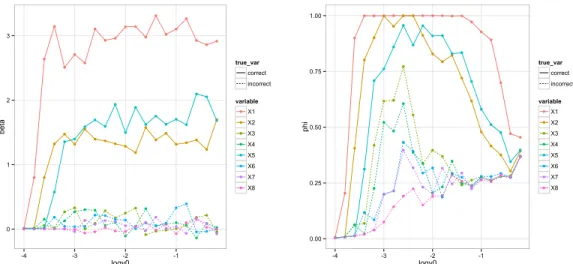
v0 varies in the logarithm scale of base 10. Only a subset of variables with high selection frequencies are displayed. . . 31 3.1 Left: The SAB path (averaged over 20 data sets) for the

posterior mean of βj for data from Simulation Study 1 with

n = 40, p = 8, and σ = 3. Right: The averaged SAB path for the inclusion probability φj. In both plots, the paths of the 3 relevant variables, X1, X2 and X5, are shown as solid lines and the paths for the other variables are shown as dashed lines. The x-coordinate denotes v0 changed in the logarithm scale of base 10. . . 46 3.2 Study 3. The SAB path for the inclusion probability φj on

the Zhao and Yu’s example, where the x-coordinate denotes

v0 changed in the logarithm scale of base 10. In this example, the true variables are X1 and X2. . . 48 3.3 Histogram of the numbers of miRNAs selected for all the

mR-NAs using the SAB algorithm. . . 52 3.4 Application of SAB to mRNA-miRNA regulation using TCGA

data. Top 50 influential miRNAs are shown. The bar lengths represent the number of mRNAs that each miRNA signifi-cantly repressed. . . 53

(9)

Chapter 1 Introduction

The emergence of advance computational technologies drives the research of statistical methodologies to extract information from massive data sets. There are two aspects of interest, learning and inference. The former is referred to model estimation, while the latter is to predict using the model. With the presence of redundant features which is common for high-dimensional data, an important task is to identify a parsimonious model that has better statistical interpretability as well as prediction accuracy. The focus of this thesis is centered around variable selection, which is a special case of model selection, to identify a subset of features that can explain well the variation in the observed response.

Variable selection has been a long-standing problem in scientific studies. The classical idea is to select variables through either sequential searching (forward, backward or step-wise) or exhausting all possible subsets by mini-mizing the combination of residual sum of square (RSS) and a penalty term such as AIC/BIC. Although conceptually straightforward, the drawbacks of such searching algorithms are well recognized: computational too expensive for high-dimensional data and prone to stuck at local optima for step-wise searching. A variety of advanced tools have been developed and investigated recently to address these issues, among which two general frameworks are adopted: penalized likelihood approach and Bayesian method, the latter be-ing the focus of my thesis. We devote the rest of this chapter to a review of these general frameworks of variable selection, leaving more detailed discus-sion of the recent work to the introduction sections of each chapter.

1.1 Penalized Likelihood Approach

Penalized likelihood approach or sometimes called the regularization method has been widely discussed and intensively used in many applications. It

(10)

identifies the relevant variable set and estimates their effects simultaneously by minimizing the combination of an empirical error (negative logarithm of the likelihood) plus a penalty term on the size of the effects.

L(θ) = −logLik(y|θ) +P enλ(θ).

The goal is to find the optimal θ that minimizes L(θ). In certain cases, the first term is also written as the residual sum of square (RSS) which alone leads to least square estimation. The second term is a penalty function indexed by a hyperparameter λ. For ease of exposition, we limit our analysis to the linear regression model with iid Gaussian errors, where the response variable yrelates to a set of potential predictorsX1, . . . , Xp in the form of a linear function. Let Xn×p denote the design matrix and βp×1 the unknown regression coefficient vector. The response y is modeled by

y∼Nn(Xβ, σ2In), where σ2 _{denotes the error variance and} _N

n denotes a n-dimensional multi-variate Normal distribution. For simplicity, set σ2 _{= 1. Then the} optimiza-tion problem of penalized likelihood approaches translates to

L(β) =||y−Xβ||2₊ p

X

j=1

P enλ(|βj|) (1.1)

A popular choice of the penalty function is the Lq penalty: P enλ(|βj|) =

λ|βj|q, whereq = 0 corresponds to the classical criteria like AIC/BIC,q = 1 the popular LASSO penalty (Tibshirani, 1996) and q = 2 resulting in ridge regression (Hoerl and Kennard, 1970). While the L0 penalty being the most essential sparsity measure strongly favors sparse solutions, it is NP-hard for optimization. The L1 penalty which is a convex relaxation of theL0 penalty, however, is more practical for implementation.

Fan and Li (2001) argued that a good penalty function should possess three properties: 1) unbiasedness, where the resulting estimator of the true effects are nearly unbiased, 2) sparsity, where the optimization procedure automatically zeros out unimportant variables and thereby leads to parsi-monious solution, and 3) continuity, that is the estimation is robust towards small perturbation of the data to avoid prediction instability. The

(11)

estima-tor of the Lq penalty is continuous if and only if q ≥ 1, but the sparsity condition is failed when q > 1. The L1 penalty on the other hand, suffers from noticeable large model bias that shifts the estimator by a constant λ. Motivated by this observation, researchers have proposed penalty functions that fulfill these three conditions, among others are the smoothly clipped absolute deviation (SCAD) penalty (Fan and Li, 2001), the minimax convex penalty (MCP) (Zhang, 2010) and the adaptive LASSO (Zou, 2006). Apart from being the guideline of a good penalty function, these appealing prop-erties also provide an insightful angle to evaluate Bayesian variable selection algorithms.

1.2 Bayesian Regularization

There is a natural connection between the penalized likelihood approach and the Bayesian framework: optimizing the penalized likelihood corresponds to the maximize-a-posteriori (MAP) process with certain prior. To be more specific, minimizing Equation (1.1) is equivalent as maximizing the following objective function:

exp{−L(β)}= exp{−||y−Xβ||2}exp{−P enλ(β)},

where the first term is proportional to the likelihood when variance σ2 is fixed, and the second term can be viewed as a prior assigned for coefficients

β. The minus logarithm of the prior distribution can be interpreted as the penalty term,

P enλ(β) =−logπ(β |λ). (1.2) For example, the LASSO penalty corresponds to the double exponential (Laplace) prior for π(β | λ) = exp{−λ|β|}, which is essentially a scale mix-ture of normals with an exponential mixing density. The Bayesian analogue to LASSO was proposed by (Park and Casella, 2008). While the frequen-tist LASSO chooses the shrinkage parameter λ by cross validation, (Park and Casella, 2008) suggested using either empirical Bayes through marginal maximum likelihood or a diffusing hyper-prior (for example Gamma prior on

λ2). Another method adapted from the recent proposed penalized likelihood approach is Bayesian Elastic net (Zou and Hastie, 2005; Li and Lin, 2010)

(12)

which uses a compromise of the Gaussian and Laplacian prior on β that is related to a mixture of the L1 and L2 penalty.

Despite the similarity, the sparsity feature of LASSO and elastic net is not transmitted to their Bayesian analogues. For variable selection, Bayesian regularization approaches need a hard shrinkage to zero out redundant vari-ables, for example the credible interval criterion and the scaled neighborhood criterion suggested in (Li and Lin, 2010).

1.3 Bayesian Hierarchical Formulation

Bayesian hierarchical model is another framework of variable selection which introduces ap-dimensional binary vectorγ = (γ1, . . . , γp)T as a model index:

γj = 1 if thejth variable is included and 0 if not. Letpγ =

P

jγj denote the size of the variable setγ,Xγ denote then×pγ design matrix which includes

only the variables entering the model γ, and βγ be the pγ ×1 vector that

corresponds to the coefficients. Then the linear model becomes:

y∼Nn(Xγβγ, σ2In).

The two key issues in this Bayesian approach are 1) the prior choice, and 2) computation of the posterior (Clyde and George, 2004). A popular choice of the prior on the model index π(γ) is the product of independent Bernoulli distributions. The conjugate Zellner’s “g-prior” (Zellner, 1986) and the “spike-and-slab” prior are widely-used for π(β | γ) the prior of the co-efficient given the model index, which is further elaborated in Section 1.3.1. After specifying the priors on all the unknowns, the Bayesian approaches make inference on the posterior distribution of γ (Zellner, 1971; Mitchell and Beauchamp, 1988; George, 2000; Liang et al., 2008) to select variables. Among a variety of posterior summary measures, two most common strate-gies are the median probability model (MPM) (Barbieri and Berger, 2004) that includes all variables withp(γj |y)>0.5, and the highest posterior den-sity (HPD) model that selects the model with the highest posterior denden-sity

(13)

1.3.1 The prior choices

In the Bayesian hierarchical formulation, a popular prior choice is the inde-pendent Bernoulli distribution for each γj,

π(γj) = Bern(θj),

where θ = (θ1, . . . , θp) is a p×1 hyper-parameter vector that contributes to small fraction of the sparsity and thereby can be used to incorporate the prior knowledge. Choosing small θ leads to a sparse solution. To give more flexibility, one can put another layer of hierarchy on the hyper-parameter θ, where the conjugate Beta prior is often used:

π(θ) =Beta(a, b).

A more general prior of the model space is π(γ) = wpγ/ _pγp

where wpγ is a prior weight put on models of size pγ (Chipman et al., 2001). Given

the model size, all possible models of the same size are equally likely. The weights wpγ reflect user’s preference on sparsity. One can put more weight on smaller size if a parsimonious solution is favored, one example being the truncated Poisson prior (Denison et al., 1998).

The prior of the coefficient β given γ has the following popular choices.

Zellner’s g-prior (Zellner, 1986) is a conjugate prior that attracted a lot attention.

p(βγ |γ, g) =Npγ(0, gσ2(XTγXγ)−1),

where g is a tuning parameter that controls the expected size of the effects. Such prior allows efficient MH algorithms for computing the posterior (George and McCulloch, 1997; Smith and Kohn, 1996), how-ever has the limitation of inconsistency in model comparison (Berger et al., 2001).

Spike-and-slab prior (Mitchell and Beauchamp, 1988) is another widely applied prior for the coefficients:

π(βj|γj) = (1−γj)δ0(βj) +γjπ1(βj),

(14)

com-ponents: the “spike” component that puts probability mass at 0 and shrinks the coefficients of all the irrelevant variables to 0, and the “slab” component that has a continuous prior distribution π1(·) and induces soft shrinkage on the large effects. In the original form, the “slab” com-ponent is a uniform diffusive distribution although other alternatives are more common for example the Gaussian distribution.

Continuous spike-and-slab prior (George and McCulloch, 1993) is a con-tinuous relaxation of the spike-and-slab prior to address the intractabil-ity issue, where the delta function is replaced by a spiky normal distri-bution.

π(βj|γj) = (1−γj)N(βj |0, v0τ2) +γjN(βj |0, v1τ2),

where v0 and v1 are two tuning parameters that control the relative size of signal and noise 0 < v0 < v1. In its original form, τ2 is a fixed hyper-parameter. (Ishwaran and Rao, 2003) suggested to assign an Inverse-Gamma (IG) prior on τ2 _{and set} _v

1 = 1 for standardized X and y in the linear regression model.

1.3.2 Connection to regularization

The Bayesian regularization methods are different from the Bayesian hierar-chical framework because they do not treat the model index as parameters nor assign prior over the model space, but make inference based on the posterior of coefficients. Albeit the difference, we can discuss the Bayesian regularization of the continuous spike-and-slab prior by translating it to a penalty function (1.2). Integrating out γj, we write the spike-and-slab prior (3.4) as a mixture of two normal distributions,

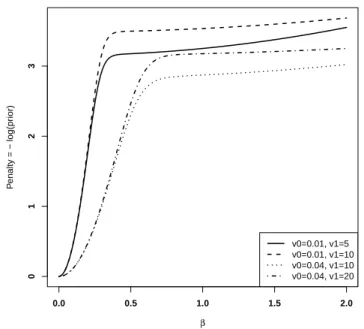
π(βj |θ, σ2) =θφ(βj; 0, v1σ2) + (1−θ)φ(βj; 0, v0σ2), (1.3) where φ(·;µ, τ2_{) denotes the pdf of} _N₍_{µ, τ}2_{). In Figure 1.1, we plot the} neg-ative logarithm of the prior in (1.3) with θ = 1/2 and σ2 = 1 for various choices of v0 and v1; we also shift the curves by logπ(0|θ, σ2) so that the penalty at βj = 0 is zero. Compared with the popular L1 penalty or equiv-alently the Double Exponential prior, the two-component normal mixture

(15)

prior (1.3) has an attractive feature from a regularization point of view: it reaches a plateau whenβ is large therefore less bias for estimation, and gives rise to a continuous approximation of the L0 penalty, although not convex. The Bayesian penalties for g-prior and the spike-and-slab prior are similar to L0 penalty like AIC/BIC.

0.0 0.5 1.0 1.5 2.0 0 1 2 3 β P enalty = − log(pr ior) v0=0.01, v1=5 v0=0.01, v1=10 v0=0.04, v1=10 v0=0.04, v1=20

Figure 1.1: A graphical display of the penalty function associated with the two-component normal mixture prior (1.3) for various choices of v0 and v1. Let β0 be the OLS estimator of the normal mean model with only one observation, β0 =y. Then the posterior mean is

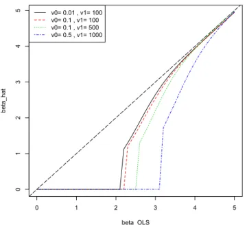
ˆ β = _E(β |β0) = φE(β |γ = 1, β0) + (1−φ)E(β |γ = 0, β0) = φ v1 1 +v1 β0+ (1−φ) v0 1 +v0 β0, s

where φ = π(γ = 1|β0), and log_1−φφ = N(β0; 0,1 +v1)/N(β0; 0,1 +v0). In Figure 1.2, we plot the truncated posterior mean ˜β = ˆβ ·1{φ≥1/2} versus the OLS estimator β0 for various choices of v0 and v1. The advantage of the Bayesian penalty is that it both returns a sparse solution and has diminishing bias, which are the desired properties discussed in (Fan and Li, 2001).

(16)

0 1 2 3 4 5 0 1 2 3 4 5 beta_OLS beta_hat v0= 0.01 , v1= 100 v0= 0.1 , v1= 100 v0= 0.1 , v1= 500 v0= 0.5 , v1= 1000

Figure 1.2: A graphical display of the truncated posterior mean ˜β in y-axis versus the OLS estimator β0 in x-axis with the two-component normal mixture prior (1.3) for various choices of v0 and v1.

1.4 Posterior Computation

1.4.1 Sampling approaches

To find out the most probable model, the exhaustive or step-wise search over the whole model space is impractical as the space size 2p _{grows too rapidly} with the dimension. Early efforts to address the scalability issue include importance sampling and brand-and-bound reduction strategies. Then the invention of MCMC techniques (including Gibbs sampler and Metropolis Hasting) brings about a proliferation of stochastic alternatives for searching the highest probability model, since a sequence of models γ(1),γ(2),γ(3), . . .

could be simulated such that their empirical distribution converges to the posteriorp(γ|y). One of the appealing features of MCMC is that it releases the close-form requirement for the posterior and thereby welcomes a wide variety of priors. However, the Metropolis Hasting using the conjugate priors is more practical, due to the advantage of rapid computation of marginal likelihood p(y|γ) in the following steps.

(17)

from the proposal distribution j(γ∗ |γ(k)_).

2. Let γ(k+1) ₌_γ∗ _{with probability below, otherwise} _γ(k+1) _remains _γ(k)_, min{1,p(y|γ

∗₎_π₍_γ∗₎

p(y|γ)π(γ) ×

j(γ |γ∗)

j(γ∗ _|_γ₎}.

Markov chain Monte Carlo model composition (MC3_{) (Madigan et al.,} 1995) is one Metropolis Hasting algorithm that proposes a new model γ∗

differing from the current γ by one variable and accept it with the rate min{1,p(_p(γ_γ∗_||_yy₎)}, which has the close-form in conjugate prior setup.

Marginalizing out the parametersβand searching over a discrete 2p _model space cause the model space approaches prone to be trapped within local peaks. Recent development to address this issue includes 1) adopting the “tempering” idea from physics that runs a population of tempered chains in parallel with flattened peaks such as Population-based MCMC (Jasra et al., 2007) and Evolutionary MCMC (Liang and Wong, 2000), and 2) combining Oscar’s Razor idea with Metropolis Hasting routine to determine a bigger set of best models such as Shortgun Stochastic Search (Hans et al., 2007).

Some other model space approaches explore the model space and the pa-rameter space simultaneously, which eases the odds of being trapped around local optima, but the difficulty is that the dimension of parameter space changes at every step. Reversible Jump MCMC (Green and Hastie, 2009) can be used to adjust the dimension of βγ dynamically. A Gibbs sampler method was proposed by (Carlin and Chib, 1995) and further extended to Gibbs variable selection (GVS) (Dellaportas et al., 2000), where a continu-ous spike-and-slab prior is used but the “spike” part is “pseudo-prior” mean-ing that the correspondmean-ing coefficients do not contribute to the predictor. Stochastic Search Variable Selection (SSVS) (George and McCulloch, 1993) is another Gibbs sampling approach on Bayesian hierarchical mixture model. Although both adopted the continuous version of spike-and-slab prior, SSVS is different from GVS in the sense that the coefficients βj givenγj = 0 of the former approach actually influence the posterior.

(18)

1.4.2 MAP estimation

Facing the increasing demand on scalability from various applications, the Bayesian approach for variable selection has one limitation, that is MCMC algorithms are computationally heavy and hard to scale with large data. In many real applications, computing the exact posterior distribution is time-consuming and unnecessary, so we turn our focus to the MAP estimation (EM algorithm) or the approximation approaches for fast solutions.

In the regularization framework, the key is to maximize a penalized likeli-hood which can be done based on the local quadratic approximation (LQA) (Fan and Li, 2001). Hunter and Li (2005) noted that LQA has a nat-ural connection with the minorization-maximization (MM) algorithm and furthermore modified LQA algorithm by adding a perturbation to render the objective function differentiable. Griffin and Brown (2005) adopted the Bayesian shrinkage prior and proposed an EM algorithm corresponding to LQA. However, there is a gap in the Bayesian hierarchical framework for the EM-like variable selection algorithm until recently Roˇckov´a and George (2014) proposed an efficient EM algorithm EMVS which adopts the continu-ous “spike-and-slab” prior on β. The continuity of the prior onβ turns out to be crucial for fast algorithms. To obtain the estimation of the model index

γ, EMVS uses a two-stage approach: first use the EM algorithm to obtain the MAP estimator of β, then use a threshold to select the desired subset of variables.

Motivated by (Roˇckov´a and George, 2014), we propose an efficient EM algorithm that can return the MAP estimator of the model indexγ directly, instead of a two-stage approach. Our EM algorithm is very fast and scales easily due to a novel computation trick that avoids inverting a large p×p

matrix in each iteration. We further proposed an ensemble version of the EM algorithm based on Bayesian bootstrap BBEM. The main idea is to repeatedly apply a stochastic version of the EM algorithm on a subset of the data (the Bayesian bootstrap samples), and then aggregate the variable selection results across the bootstrap samples to improve the accuracy. The details are given in Chapter 2.

(19)

1.4.3 Approximation approaches

The MAP procedure is very fast in computation but only provides a point estimation. When the full posterior distribution is preferred, we consider the approximation approaches. Variational Bayes (VB) and Expectation prop-agation (EP) are two closely-related techniques for posterior approximation yet show advantages in different scenario. The approximation approaches introduce a factorized distribution Q and update each component in Q se-quentially to minimize the Kullback-Leibler (KL) divergence between Qand the true posterior P until convergence. The KL divergence (Kullback and Leibler, 1951) is a non-negative, asymmetric metric defined as:

KL(P||Q) =

Z

P(x) logP(x)

Q(x)dx.

A fundamental difference between VB and EP is that the objective func-tion of the former approach is KL(Q||P) whereas the latter working on

KL(P||Q). Other extensions include power EP (Minka, 2004) that based on the α-divergence: Dα(P||Q) = 1 α(1−α) 1− Z P(x)αQ(x)(1−α)dx ,

with α →0 corresponding to VB, α → 1 corresponding to EP and α = 0.5 corresponding to the Hellinger distance.

In the context of linear model, with the variance parameter σ2 and the Bernoulli parameter θ fixed, the full posterior is

π(γ,β |y)∝p(y|β)π(β |γ)π(γ).

The EP approach factorizes Q by:

Q(γ,β) = n Y i=1 qi(yi,β) p Y j=1 qj(βj, γj)q(γ)

where qi(yi,β), qj(βj, γj) and q(γ) correspond to the likelihood term p(yi |

β), the prior π(βj) and π(γ) respectively. Hern´andez-Lobato et al. (2010, 2013) introduced an efficient EP algorithm for multi-task feature selection and group feature selection that use a generalized spike-and-slab prior with

(20)

a point mass component. Recently, Andersen et al. (2014) proposed another EP framework for Bayesian feature selection that uses a structured spike-and-slab prior to incorporate the prior knowledge of the sparsity pattern. Carbonetto et al. (2012) introduced a VB approach for variable selection that adopts the original spike-and-slab prior and factorizesQin the following form, Q(γ,β) = p Y j=1 q(βj, γj).

The use of the point mass component demands the dependency of βj andγj in Q due to the non-conjugate prior.

In Chapter 3, we propose a hybrid framework of VB and EM for scalable Bayesian variable selection called SAB that adopts the continuous spike-and-slab prior. Unlike (Carbonetto et al., 2012), we factorize the approximate function Q in the following way,

Q(γ,β) =q(β) p

Y

j=1

q(γj).

The optimal q(β) and q(γj) are in the multivariate Normal family and the Bernoulli family respectively, which are conjugate to the priors. In this ap-proach, we assume independence between β and γ for the approximate pos-terior, which entails Q cannot be as close as to P but the convergence is guaranteed due to convexity. Instead of reporting just a single model, the SAB algorithm returns the posterior probabilities of γ, which provides more flexibility on model inference such as model ranking, FDR control and model averaging.

As a trade-off between computation cost and accuracy, we do not expect that the VB algorithm obtains the exact posterior distribution like MCMC methods. Instead we are looking for a good approximation of the posterior distribution. Here by “good”, we mean that the result from SAB, albeit an approximation, achieves the desired asymptotic properties, such as the selection consistency and the oracle property. The asymptotic analysis of the SAB algorithm for high dimensional data (p > n) is given in Chapter 4.

(21)

1.5 Extension to Generalized Linear Model

In Chapter 5, we discuss the extension of our Bayesian variable selection framework to the Generalized Linear Model (GLM). Logistic regression is the most commonly used method to model binary response data. But trans-forming the nicely-built algorithms from linear regression to logistic model is not always straightforward. In the Bayesian framework, the difficulty mainly comes from the non-conjugate likelihood. Several solutions have been pro-posed from one of the three basic ideas: the MAP estimation, sampling algorithms or approximation approaches. To be more specific, the MAP pro-cedure provides a point estimator which is fast but surely misses out some information of the whole posterior. The sampling method uses a Metropo-lis Hasting algorithm to sample from the posterior, which is more accurate and informative but notorious for its slow mixing time. The approximation approach, on the other hand, uses different factorization functions (often connect to the exponential family) to approximate the posterior, for example the probit approximation or Laplace approximation.

A recent work by (Polson et al., 2013) introduced an auxiliary variable from Polya-Gamma distribution in the GLM specification. Given that auxiliary variable, the logistic likelihood is valued as Normal densities, which bypasses the non-conjugate issue so that the parameters and latent variables can be updated using an EM algorithm. But in the scenario of variable selection, this method has a drawback, that is for sparse data, if a variable with small coefficient estimation is deleted, it cannot reenter the model.

Based on the Polya-Gamma method, we propose a hybrid framework of VB and EM for logistic variable selection that adopts the continuous spike-and-slab prior in Chapter 5. We also show an equivalence between the Polya-Gamma method and the local approximation method (Bishop, 2006) for VB in logistic model.

(22)

Chapter 2 EM and Ensemble

2.1 Introduction

Consider a simple linear regression model with Gaussian noise:

y=Xβ+e (2.1)

where y = (y1, . . . , yn)T is the n×1 response, e = (e1, . . . , en)T is a vector of iid Gaussian random variables with mean 0 and variance σ2_{, and}_X_{is the}

n×pdesign matrix. The unknown parameters are the regression parameter

β = (β1, . . . , βp)T and the error varianceσ2. In many real applications such as bioinformatics and image analysis, where linear regression models have been routinely used, the number of potential predictors (i.e., p) is large but only a small fraction of them is believed to be relevant. Therefore the linear model (2.1) is often assumed to be “sparse” in the sense that most of the coefficients

βj’s are zero. Estimating the set of relevant variables,S ={j :βj 6= 0}is an important problem in modern statistical analysis.

The Bayesian approach to variable selection is conceptually simple and straightforward. First introduce ap-dimensional binary vectorγ = (γ1, . . . , γp)T to index all the 2p sub-models, where γj = 1 if the jth variable is included in this model and 0 if excluded. Usually γj’s are modeled by independent Bernoulli distributions. Given γ, a popular prior choice for β is the “spike and slab” prior (Mitchell and Beauchamp, 1988):

π(βj |γj) =    δ0(βj), if γj = 0; g(βj), if γj = 1, (2.2)

whereδ0(·) is the Kronecker delta function corresponding to the density func-tion of a point mass at 0 and g is a continuous density function. After

(23)

specifying priors on all the unknowns, one needs to calculate the posterior distribution. Most algorithms for Bayesian variable selection rely on MCMC such as Gibbs or Metropolis Hasting to obtain the posterior distribution; for a review on recent developments in this area, see O’Hara and Sillanp¨a¨a (2009). MCMC algorithms, however, are insufficient to meet the growing de-mand on scalability from real applications. Since the primary goal is variable selection, we focus on efficient algorithms that return the MAP estimate of

γ, as an alternative to these MCMC-based sampling methods that return the whole posterior distribution on all the unknown parameters.

Recently, Roˇckov´a and George (2014) proposed a simple, elegant EM al-gorithm for Bayesian variable selection. They adopted a continuous version of the “spike and slab” prior—the spike component in (2.2) is replaced by a normal distribution with a small variance (George and McCulloch, 1993), and proposed an EM algorithm to obtain the MAP estimate of the regres-sion coefficient β. The MAP estimate ˆβMAP, however, is not sparse, so an additional thresholding step is needed to estimate γ.

In this chapter, we develop an EM algorithm that directly returns the MAP estimate of γ, so no further thresholding is needed. We adopt the same continuous “spike and slab” prior. Different from the algorithm by Roˇckov´a and George (2014) that returns ˆβMAP by treating γ as latent, our algorithm returns the MAP estimate of the model index, ˆγMAP, by treating

β as latent. The special structure of our EM algorithm allows us to use a computational trick to avoid inverting a big matrix at each iteration, which seems unavoidable in the algorithm by Roˇckov´a and George (2014). Further we can show that the ˆγMAP achieves asymptotic consistency even when p diverges to infinity with the sample size n.

Although shown to achieve selection consistency, in practice, our EM al-gorithm could get stuck at a local mode due to the large discrete space in which γ lies. Borrowing the idea of bagging, we propose an ensemble version of our EM algorithm (which we call BBEM): apply the algorithm on multiple Bayesian bootstrap (BB) copies of the data, and then aggregate the variable selection results. Bayesian bootstrap for variable selection was explored be-fore by Clyde and Lee (2001) for the purpose of prediction, where models built on different bootstrap copies are combined to predict the response. But the focus of our approach is to summarize the evidence for variable relevance from multiple BB copies, which is similar in nature to several frequentist

(24)

ensemble methods for variable selection, such as the AIC ensemble (Zhu and Chipman, 2006), stability selection (Meinshausen and B¨uhlmann, 2010), and random Lasso (Wang et al., 2011).

The remaining of the paper is organized as follows. Section 2 describes the EM algorithm in detail, Section 3 presents the asymptotic results, and Section 4 describes the BBEM algorithm. Empirical studies are presented in Section 5 and conclusions and remarks in Section 6.

2.2 Method

2.2.1 Prior specification

We adopt the continuous version of “spike and slab” prior for β, i.e. a mixture of two normal components with mean zero and different variances:

π(βj |σ, γj) =    N(0, σ2_v 0), if γj = 0; N(0, σ2_v 1), if γj = 1, (2.3)

where v1 > v0 >0. Alternatively, we can write the prior on β as

π(βj |σ2, γj) =N(0, σ2dγj),

where

dγj =γjv1+ (1−γj)v0.

The choice of tuning parameters v0 and v1 is discussed in Section 2.5. For the remaining parameters, we specify independent Bernoulli priors on elements of γ, and conjugate priors like Beta and Inverse Gamma on θ and

σ2_{, respectively:}

π(γ |θ) = Bern(θ), π(θ) = Beta(a0, b0),

π(σ2) = IG(ν0/2, ν0λ0/2).

(25)

choices unless prior knowledge is available:

a0 =b0 = 1.1, ν0 =λ0 = 1. (2.4)

2.2.2 The EM algorithm

With the Gaussian model and prior distributions specified above, we can write down the full posterior distribution:

π(γ,β, θ, σ2 |y) ∝ p(y|β, σ2)×π(β |σ,γ)×π(γ |θ)×π(θ)×π(σ2).

Treating β as the latent variable, we derive an EM algorithm that returns the MAP estimation of parameters Θ = (γ, σ2, θ), whereas the roles ofβand

γ are switched in Roˇckov´a and George (2014).

E Step

The objective functionQat the (t+ 1)-th iteration in an EM algorithm is de-fined as the integrated logarithm of the full posterior with respect to βgiven

+ logπ(θ) + logπ(σ2) + Constant is a function of Θ not depending on β.

It is easy to show that β follows a Normal distribution with mean m and covariance matrix σ_(t)2 V, given Θ(t) and y, where

m = V−1XTy, V = XTX+D_γ−1(t) −1 , (2.6) D_γ(t) = diag d_γ(t) j p j=1 = diagγ_j(t)v1+ (1−γ (t) j )v0 p j=1 .

(26)

Then the two expectation terms in (2.5) can be expressed as: Eβ|Θ(t)_,_y y−Xβ 2 = σ_(t)2 tr(XVXT) +y−Xm 2 , (2.7) Eβ|Θ(t)_,_y p X j=1 β2 j dγj = p X j=1 σ_(t)2 Vjj +m2j (1−γ_j(t))v0+γ (t) j v1 . (2.8) M Step

We sequentially update parameters (γ, θ, σ) to maximize the objective func-tion Q.

1. Update γj’s. The terms involving γj in (2.5) are

− 1 2σ2 (t) Eβ|Θ(t)_,_y _β2 j dγj − 1 2logdγj+ logπ(γj |θ (t)₎_. _(2.9)

Plug in γj = 0 andγj = 1 to (2.9) respectively, then we have

γ_j(t+1) = 1, if _E_β|Θ(t)_,_y β_j2 > r(t), (2.10) where r(t) = σ 2 (t) 1/v0−1/v1 logv1 v0 −2 log θ (t) 1−θ(t) .

2. Update (σ2_{, θ}₎_._Given_γ(t+1)_{, the updating equations for the other two} parameters are given by

σ_(t+1)2 = Eβ |Θ(t)_,_y h ky−Xβk2₊Pp j=1β 2 j/d_γ(t+1) j i +v0λ0 n+p+v0 , (2.11) θ(t+1) = Pp j=1γ (t+1) j +a0−1 p+a0+b0−2 . (2.12) Stopping Rule

The EM algorithm alternates between the E-step and M-step until conver-gence. A natural stopping criterion is to check whether the change of the objective functionQ is small. To reduce the computation cost for evaluating the Qfunction, we adopt a different stopping rule as our main focus isγ: we stop our algorithm when the estimate γ(t) _{stays the same for} _k

(27)

In practice, we suggest to set k0 = 3.The pseudo code of this EM algorithm is summarized in Algorithm 1.

Algorithm 1: EM Algorithm

Input: X,y, v0, v1, a0, b0, ν0, λ0 Initialize Θ(0)_;

E-step: Calculate the two expectations in (2.7) and (2.8), denoted as

EE(0)_;

for t = 1 : maxIter do

M-step: Update Θ(t) _{from Eq (2.10, 2.11,teq:the1);} E-step: Update EE(t) _{from Eq (2.7, 2.8);}

if γ(t) _{stays the same for} _k

0 = 3 iterations then break; end end Returnγ, m,V;

2.2.3 Computation cost

At each E-step, updating the posterior of β given other parameters in (2.6) requires inverting a p×p matrix

V(t) = (XTX+D−1_γ(t))

−1

, (2.13)

which is the major computational burden of the algorithm. When p > n, we can use the Sherman-Morrison-Woodbury formula to compute the inverse of an n ×n matrix. So the computation cost at each iteration is of order

O(min(n, p)3_{). It is, however, still time-consuming when both} _n _and _p _are large.

Note that the only thing that changes in (2.13) from iteration to iteration is D_γ(t), a diagonal matrix depending on the binary vector γ(t). From our

experience, only a small fraction of γ_j(t)’s are changed at each iteration after the first a couple of iterations. So the idea is to use the following recursive formula to compute V(t): V(t) = (XTX+D−1_γ(t−1) +D −1 γ(t) −D −1 γ(t−1)) −1 = (V−1_(t−1)+D_γ−1(t) −D −1 γ(t−1)) −1 (2.14)

(28)

whereD−1

γ(t)−D

−1

γ(t−1) is a diagonal matrix with the j-th diagonal entry being

non-zero only if the inclusion/exclusion status, i.e., the value ofγj, is changed from the last iteration. Let ldenote the number of variables whose γj values are changed from iteration (t−1) tot. ThenD−1_γ(t)−D

−1

γ(t−1) is a ranklmatrix.

We can apply the Woodbury formula on (2.14) to reduce the computation complexity from O(min(n, p)3_{) to} _O₍_l3_).

For example, without loss of generality, suppose only the firstl covariates have their γj values changed. Then, we can write

D−1_γ(t) −D −1 γ(t−1) =Up×lAl×lU T_, where A = _v1 0 − 1 v1 diag(2γ_j(t)−1)l

j=1 and U consists of the first l columns from Ip. Applying the Woodbury formula, we have

V(t) =V(t−1)−V(t−1)U(A−1+UTV(t−1)U)−1UTV(t−1).

2.3 Asymptotic Analysis

In this section, we study the asymptotic property of ˆγn, the MAP estimate of model index returned by our EM algorithm. Assume the data yn are generated from a Gaussian regression model:

yn∼Nn Xnβn∗, σ 2_I

n

.

Here we consider a triangular array set up: the dimension p = pn diverges with n and the true coefficient β∗_n also vary withn. Suppose the true model is indexed by γ_n∗, where γ_nj∗ = 1 if β_nj∗ 6= 0 and γ_nj∗ = 0 if β_nj∗ = 0. We show that our EM algorithm has the following selection consistency property:

P(ˆγn =γn∗)→1, asn → ∞.

First we list some regularity conditions needed in our proof. Let λmin(A) denote the smallest eigenvalue of matrix A. We assume

(A1) On collinearity: let λmin(A) denote the smallest eigenvalue of matrix

A,

(29)

In the traditional asymptotic setting where p is fixed, we have η1 = 1. (A2) On sparsity:

kβ_n∗k2 =O(nη2), 0< η2 < η1,

which controls the L2 norm of the true regression coefficient vector. (A3) The beta-min condition:

lim inf n min |β∗ nj|, γ ∗ nj = 1 n(η3−1)/2 ≥M, 0≤η3 <1,

where M is a positive constant. This condition requires that the mini-mal non-zero coefficient cannot go to zero at a rate faster than 1/√n. In the traditional asymptotic setting whereβ∗_nis fixed, we haveη3 = 0. (A4) On hyper-parameters: assume log[ˆθn/(1−θˆn)] and ˆσ2n are bounded.

This condition is purely technical for the simplicity of the proof. To sat-isfy this condition, we could fix ˆθnand ˆσnat constant or set a threshold to avoid them going to extreme. In simulations, we recommend (2.4) as the choice for hyper-parameters unless p is large.

(A5) On tuning parameters: assumev1 is fixed at constant andv0 satisfies 0< v0 =O(n−r0), 1−η3 < r0 <min n η1−α, 2 3(η1−η2) o ,

where 0< α <1 is the rate of the dimension p=O(nα_).

Theorem 2.1. Assume (A1-A5) and p = O(nα) where 0 ≤ α < 1, then the model returned by our EM algorithm, γˆn, achieves the following selection

consistency,

P(ˆγn=γn∗)→1, as n→ ∞. (2.15)

Proof. See Appendix.

2.4 Bayesian Bootstrap

A common issue with EM algorithms is that they could be trapped at a local maximum. There are some standard remedies available for dealing with this issue, for instance, trying a set of different initial values or utilizing some more

(30)

advanced optimization procedures at the M-step. Since our EM algorithm is searching for the optimal γ over a big discrete space, all p-dimensional binary vectors, these remedies are less useful when p is large.

When doing optimization with γ, a discrete vector, the resulting solution is often not stable, i.e., has a large variance. Bagging is an easy but power-ful method (Breiman, 1996) for variance reduction, which applies the same algorithm on multiple bootstrap copies of the data, and then aggregates the final results. We proposed the following ensemble EM algorithm, in which we repeatedly run the EM variable selection algorithm, Algorithm 1 from Section 2.2.2, on Bayesian bootstrap replicates.

The original bootstrap repeatedly samples data from the original data set

{(xi, yi)}ni=1 with replacement, i.e., each observation (xi, yi) is sampled with probability 1/n.In Bayesian bootstrap (Rubin, 1981), instead of sampling a subset of the data, we assign a random weight wi to the i-th observation and then fit a weighted least squares regression model on the whole data set. In particular, following Rubin (1981), we generate the weightsw= (w1, . . . , wn) from a n-category Dirichlet distribution:

wn×1 ∼Dir(1,· · · ,1). (2.16) When applying Algorithm 1 on a weighted linear regression model, all the updating equations stay the same, except the updating equation (2.6) for the posterior of β, which should be changed to:

m=VXTdiag(w)y, V= (XTdiag(w)X+D_γ−1(t))

−1

. (2.17)

Eq (2.7), the expectation of the weighted residual sum of squares, should also be changed accordingly: Eβ|Θ(t)_,_y y−Xβ 2 w =σ 2 (t)tr(diag(w)XVX

T₎₊₍_y−Xm₎T_diag(_w₎₍_y−Xm₎_. (2.18) It is well-known that in order to make the aggregation work, we should control the correlation among estimates from bootstrap replicates. For ex-ample, in random forest (Breiman, 2001), the number of variables used for choosing the optimal split of a tree is restricted to a subset of the variables, instead of using all pvariables. A similar idea was implemented in Random

(31)

Lasso (Wang et al., 2011), an ensemble algorithm for variable selection. In the same spirit, we apply the EM algorithm only on a subset of the variables at each Bayesian bootstrap iteration. A naive way is to randomly pick a subset from thepvariables. This, however, will be inefficient when pis large and the true model is sparse, since it is likely most random subsets will not contain any relevant variables. So we employ a biased sampling procedure: sample the p variables based on a weight vector ˜π that is defined as

˜

πp×1 ∝ |XTy|/diag(XTX), (2.19) that is, variables are sampled based on their marginal effect in a simple linear regression.

The ensemble EM algorithm operates as follows. First we sample a random set of L variables according to the probability vector ˜π, and draw a n ×1 bootstrap weight vector w from (2.16). Let ˜X be the new data matrix with the L columns. Then apply the EM algorithm on the bootstrap replicate

˜

X with weight w. Let γk denote the model returned by the k-th Bayesian bootstrap iteration, where the j-th position of γk is 1 if the j-th variable is selected and zero otherwise; of course, the j-th position is zero if the j-th variable is not included in the initial L variables. Define the final variable selection frequency for the p variables as

φp×1 = 1 K K X k=1 γk. (2.20)

We can report the final variable selection result by thresholdingφj’s at some fixed number, for example, a half. Or we can produce a path-plot of φ as

v0 varies, which could be a useful tool to investigate the importance of each variable. We illustrate this in our simulation study in Section 2.5.

As for the computational cost, the inversion of theL×Lmatrix in (2.17) is a big improvement compared with that of a p×pmatrix. By the same logic as in Section 2.2.3, it can be further simplified to inverting a l-by-l matrix, where l is the number of variables that changes their inclusion status, and l ¡ L. The complete BBEM algorithm is summarized in Algorithm 2.

(32)

Algorithm 2: BBEM Algorithm

Input: X,y, v0, v1, a0, b0, ν0, λ0, K, L

Compute the variable weight ˜π from (2.19);

for k = 1 : K do

Generate a subset ofL variables according to ˜π; Make the replicate ˜Xk with the L variables; Initialize Θ(0)_k ;

Generate bootstrap weightw from (2.16);

E-step: Calculate the two expectations in (2.8), denoted as EE_k(0);

for t = 1 : maxIter do

M-step: Update Θ(t)_k from Eq (2.10, 2.11, 2.12); E-step: Update EE_k(t) from Eq (2.17, 2.18);

if γ_k(t) stays the same for k0 = 3 iterations then break; end end Recordγ_k(t); end Returnφ from Eq (2.20);

2.5 Empirical Results

In this section, we first compare the proposed EM algorithm (Algorithm 1) with other popular methods on a widely used benchmark data set. Then we compare BBEM (Algorithm 2) with other methods on two more challenging data sets of larger dimensions. Finally, we applied BBEM on a restaurant revenue data from a Kaggle competition, and showed that our algorithm outperforms the benchmark from random forest.

For the hyper-parameters v0 and v1, we set v1 = 100 as fixed and tune an appropriate value for v0 either based on 5-fold cross-validation or BIC. For the initial value of θ, we suggest to use 1/2 for ordinary problems, but

√

n/p for large-p problems. Given θ(0)_{, the initial value of the binary vector}

γ(0) _{is randomly generated from Bernoulli distribution with parameter} _θ(0)_. The initial value of σ2 is set as 1. In addition, there are two bootstrap parameters: the total number of replicates K and the number of variables used in each bootstrap L. For efficiency, the number of variables in each bootstrap replicate should not exceed the sample size n. We use K = 100, and L=n/2 if p is large andL=p isp is small.

(33)

2.5.1 A widely used benchmark

First we apply our EM algorithm on a widely used benchmark data set (Tibshirani, 1996), which has p = 8 variables, each from a standard nor-mal distribution with pairwise correlation ρ(xi,xj) = 0.5|i−j|. The response variable is generated from

y= 3x1+ 1.5x2+ 2x5+ where ∼N(0, σ2_).

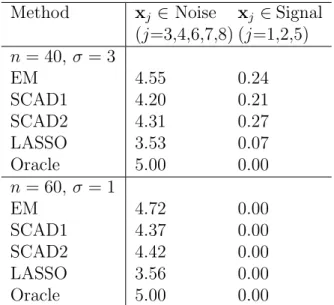
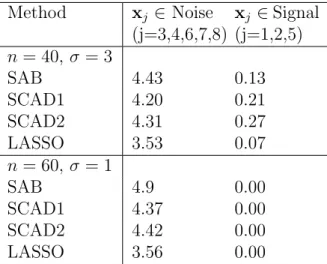
Following Fan and Li (2001), we repeat the experiment 100 times under two scenarios: (1) n = 40, σ = 3 and (2) n = 60, σ = 1. The result is shown in Table 2.1, which reports the average number of zero-coefficients (i.e., no selection) among signal variables (x1,x2,x5) and among noise vari-ables, respectively. The results for SCAD1 (tuning parameter selected by cross-validation), SCAD2 (tuning parameter fixed) and LASSO are taken from (Fan and Li, 2001). In the first “small sample-size high noise” scenario, our EM algorithm has the highest number of zero-coefficients among noise variables, i.e., the lowest type I error. The average number of signal variables missed by EM is slightly higher than SCAD1 (where the tuning parameter is chosen by cross-validation) but less than SCAD2 (where the tuning parame-ter is pre-fixed). But overall, our EM algorithm and the two SCAD methods perform the best. In the second “large sample-size low noise” scenario, no signal variables are missed by any method, but EM has the lowest type I error.

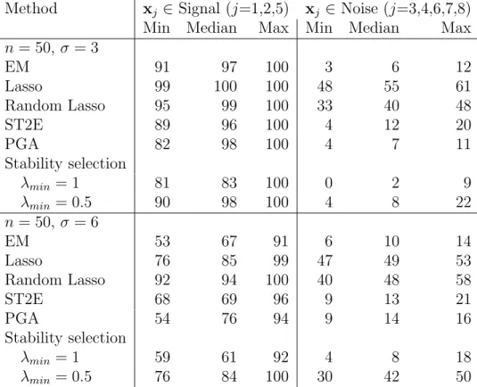
Following (Wang et al., 2011) and (Xin and Zhu, 2012), we repeat the experiment 100 times with the same sample size n = 50 but two different noise levels: low noise level (σ = 3) and high noise level (σ = 6). Table 2.2 reports the minimum, median, maximum of being selected out of 100 simulations for the signal and the noise variables, respectively. Both Lasso and random Lasso have a higher chance of selecting the signal variables, but at the price of mistakenly including many noise variables. Overall, our EM algorithm performs the best, along with PGA and stability selection, two frequentist ensemble methods for variable selection.

(34)

Method xj ∈ Noise (j=3,4,6,7,8) xj ∈Signal (j=1,2,5) n = 40, σ= 3 EM 4.55 0.24 SCAD1 4.20 0.21 SCAD2 4.31 0.27 LASSO 3.53 0.07 Oracle 5.00 0.00 n = 60, σ= 1 EM 4.72 0.00 SCAD1 4.37 0.00 SCAD2 4.42 0.00 LASSO 3.56 0.00 Oracle 5.00 0.00

Table 2.1: A widely used benchmark. The average number of

zero-coefficients (i.e., no selection) out of 100 simulations for each types of variable (Signal or Noise) are shown. The results other than EM (Alg 1) are from (Fan and Li, 2001).

2.5.2 A highly-correlated data

Next we demonstrate our two algorithms on a highly-correlated example from (Wang et al., 2011). The data has p = 40 variables and the response y is generated from

y= 3x1+ 3x2−2x3+ 3x4+ 3x5−2x6+, where ∼ N(0, σ2_{) and} _σ _{= 6. Each} _x

i is generated from a standard nor-mal with the following correlation structure among the first six signal vari-ables: the signal variables are divided into two groups, V1 ={x1,x2,x3} and

V2 ={x4,x5,x6}; the within group correlation is 0.9 and the between-group correlation is 0.

We repeat the simulation 100 times with n = 50 and n = 100, and the results are summarized in Table 2.3. For this example, due to the high correlation among features we expect ensemble methods to perform better. Indeed, BBEM has the best performance in terms of selecting true signal variables while controlling the error of including noise variables. The per-formance of EM algorithm, although not the best, is also comparable with other top ensemble methods like random Lasso from (Wang et al., 2011), and

(35)

Method xj ∈ Signal (j=1,2,5) xj ∈ Noise (j=3,4,6,7,8)

Min Median Max Min Median Max

n= 50, σ = 3 EM 91 97 100 3 6 12 Lasso 99 100 100 48 55 61 Random Lasso 95 99 100 33 40 48 ST2E 89 96 100 4 12 20 PGA 82 98 100 4 7 11 Stability selection λmin = 1 81 83 100 0 2 9 λmin = 0.5 90 98 100 4 8 22 n= 50, σ = 6 EM 53 67 91 6 10 14 Lasso 76 85 99 47 49 53 Random Lasso 92 94 100 40 48 58 ST2E 68 69 96 9 13 21 PGA 54 76 94 9 14 16 Stability selection λmin = 1 59 61 92 4 8 18 λmin = 0.5 76 84 100 30 42 50

Table 2.2: A widely used benchmark. The min, median, max number of being selected out of 100 simulations for each types of variable (Signal or Noise) are shown. The results other than EM (Alg 1) are from (Xin and Zhu, 2012).

T2E and PGA from (Xin and Zhu, 2012).

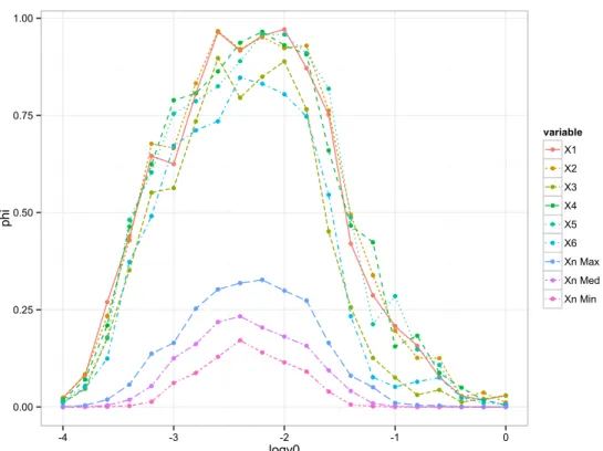
For illustration purpose, we apply BBEM on a data set with n = 50 and

v0 varying from 10−4 to 1. Figure 2.1 shows the path-plot of the selection frequency from BBEM. There is clearly a gap between the signal variables and the noise ones. For a range of v0, from 0.001 to 0.02, BBEM can successfully select the six true variables {x1,x2, . . . ,x6} if we threshold the selection frequency φj at 0.5.

Unlike the trumpet shape in LASSO, Figure 2.1 shows a hat shape for BBEM. Whenv0 is extremely small, the “spike” component is close to point mass at 0. Intuitively, any nonzero coefficient should not be clustered to a point mass component. But in the update equation (2.6), we find that the posterior mean and variance of the coefficient β shrinkage to 0 very quickly for small v0. In the update equation (2.10) for γj, the second moment of βj (left hand side) goes to zero faster than the threshold (right hand side). This

(36)

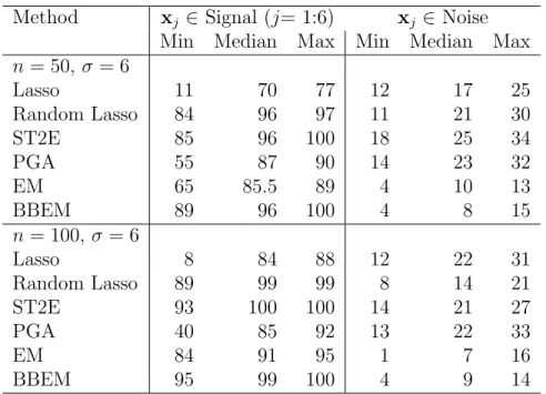
Method xj ∈ Signal (j= 1:6) xj ∈Noise Min Median Max Min Median Max

n = 50, σ= 6 Lasso 11 70 77 12 17 25 Random Lasso 84 96 97 11 21 30 ST2E 85 96 100 18 25 34 PGA 55 87 90 14 23 32 EM 65 85.5 89 4 10 13 BBEM 89 96 100 4 8 15 n = 100,σ = 6 Lasso 8 84 88 12 22 31 Random Lasso 89 99 99 8 14 21 ST2E 93 100 100 14 21 27 PGA 40 85 92 13 22 33 EM 84 91 95 1 7 16 BBEM 95 99 100 4 9 14

Table 2.3: A highly-correlated data. The min, median, max number of times being selected (i.e., no selection) out of 100 simulations for each type of variables (Signal and Noise) are shown. The results other than EM and BBEM are from (Xin and Zhu, 2012).

explains why the BBEM algorithm labels every variable as “not included” when v0 goes too small.

2.5.3 A Large-

p

small-

n

example

Finally we apply BBEM on a large-p small-n example from (Roˇckov´a and George, 2014), where p = 1000 and n = 100. Each of the p features is generated from a standard normal with pairwise correlation to be 0.6|i−j| and the response yis generated from the following linear model:

y=x1+ 2x2+ 3x3+, where ∼N(0,3).

For this large p example, we set the parameters in the BBEM algorithm as follows: the initial value of θ is √n/p, the number of variables used in each bootstrap iteration L = n/2 = 50 and the total number of replicates

K = 100. It is shown that cross-validation based on prediction accuracy tends to include more noise variables (Wang et al., 2007). So, for this example where the true model is known to be sparse, we choose to tunev0 via BIC. For

(37)

0.00 0.25 0.50 0.75 1.00 -4 -3 -2 -1 0 logv0 phi variable X1 X2 X3 X4 X5 X6 Xn Max Xn Med Xn Min

Figure 2.1: Highly-correlated data n = 50. A path-plot of the average selection frequency when v0 varies in the logarithm scale of base 10. Top 6 lines represent the true variables x1:6 and the bottom 3 lines represent the maximum, median and minimum among the noise variables x7:40.

illustration purpose, we also include BBEM with a fixed tuning parameter

v0 = 0.03 in the comparison group. We compare BBEM with the EMVS algorithm from (Roˇckov´a and George, 2014), which is implemented by us using the annealing technique for β’s initialization, and fixed v0 = 0.5, v1 = 1000 as suggested in (Roˇckov´a and George, 2014).

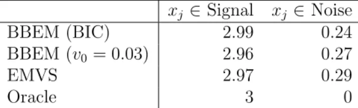
Table 2.4 reports the average number of signal and noise variables being se-lected over 100 iterations for each method. BBEM with BIC tuning performs the best: it selects 2.99 signal variables out of 3 on average (i.e., only miss one variable, the weakest signalx1, once in all 100 iterations) and meanwhile has the smallest type I error. The BBEM algorithm with a fixed tuning pa-rameter has a similar result as EMVS but is much faster. The computation advantage for BBEM comes from two aspects: the computation trick that reduces the computation cost on matrix inversion and the sub-sampling step in Bayesian bootstrap which allows us to deal with just a subset of variables of size smaller than p.

(38)

xj ∈ Signal xj ∈Noise

BBEM (BIC) 2.99 0.24

BBEM (v0 = 0.03) 2.96 0.27

EMVS 2.97 0.29

Oracle 3 0

Table 2.4: A large-psmall-n example. The table shows the average number of signal and noise variables being selected out of 100 iterations. In BBEM,

v0 is either chosen by BIC or fixed at 0.03. EMVS is the algorithm proposed by Roˇckov´a and George (2014).

2.5.4 A real example

For TFI, a company that owns some of the world’s most well-known brands like Burger King and Arby’s, decisions on where to open new restaurants are crucial. It usually takes a big investment of both time and capital at the beginning to set up a new restaurant. If a wrong location is chosen, likely the restaurant will soon be closed and all the initial investment will be lost. TFI hosted a prediction competition on Kaggle1_{, where the goal is} to build a mathematical model to predict the revenue of a restaurant based on a set of demographic, real estate, and commercial information. The data contains 137 restaurants in the training set and 1000 restaurants in the test set. Features include the Open Date, City, City Group, Restaurant Type, and three categories of obfuscated data (P1-P37, numeric): demographic data, real estate data, and commercial data. The response is the transformed restaurant revenue in a given year.

We first transform the “Open Date” to a numeric feature called “Year Since 1900” and merge the “City” column into the “City Group” column which now contains four categories: Istanbul, Izmir, Ankara, and others (small cities). Then we crate dummy variables for the categorical features like “City Group” and “Restaurant Type” and keep all the obfuscated numeric columns P1-P37. The final training set has 43 features and 137 samples.

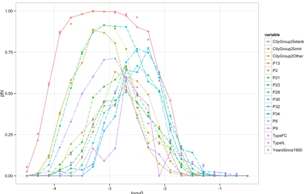
After standardizing the data, we fix v1 at 100 and tune v0 from 10−4.5 to 10−0.5 for the BBEM algorithm, where each bootstrap sample uses L = 15 variables, and the total number of replicates is K = 300. The path-plot of selection frequency for important features is shown in Figure 2.2. It is not surprising that “City Group”, “Years Since 1900” and “Restaurant Type” are

1

(39)

some important predictors for the revenue. Quite a few obfuscated features are also selected as important predictors. Although we do not know their meanings, they should provide valuable information for TFI to choose their next restaurant’s location.

0.00 0.25 0.50 0.75 1.00 -4 -3 -2 -1 logv0 phi variable CityGroup2İstanbul CityGroup2İzmir CityGroup2Other P13 P2 P21 P23 P28 P30 P32 P34 P6 P9 TypeFC TypeIL YearsSince1900

Figure 2.2: Restaurant data. The path plot of selection frequency when v0 varies in the logarithm scale of base 10. Only a subset of variables with high selection frequencies are displayed.

Since the evaluation metric for this specific competition is based on the rooted mean square error (RMSE), we use the same metric in our 5-fold

cross-validation. We tunedv0from the set{0.0001,0.0002,0.0005,0.001,0.002,0.005,0.01}, and found v0 = 0.002 has the smallest RMSE score. Then we fixv0 at 0.002,

and re-run BBEM on the whole training data. Let m denote the averaged posterior mean ofβfromLbootstrap iterations, andγthe averaged selection frequency for p variables. We then usem∗γ (where∗ denotes element-wise product) for prediction in the same spirit as the Bayesian model averaging. Our final Kaggle score is 1989762.52, which outperforms the random forest benchmark (RMSE=1998014.94) provided by Kaggle2. It is remarkable for

2_{At Kaggle, each team can submit their prediction and see the corresponding}

perfor-mance on the test data many times, so one can easily obtain a good score by keep tweaking the model to overfit the test data. For this reason, we did not compare our result with

(40)

BBEM to outperform random forest considering that BBEM does not use any nonlinear features but random forest does.

2.6 Discussion

Variable selection is an important problem in modern statistics. In this chapter, we study the Bayesian approach to variable selection in the context of multiple linear regression. We proposed an EM algorithm that returns the MAP estimate of the set of relevant variables. The algorithm can be operated very efficiently and therefore can scale up with big data. In addition, we have shown that the MAP estimate from our algorithm provides a consistent estimator of the true variable set even when the model dimension diverges with the sample size. Further, we propose an ensemble version of our EM algorithm based on Bayesian bootstrap, which, as demonstrated via real and simulated examples, can substantially increase accuracy while maintaining the computation efficiency.

Although we restrict our discussion for the linear model, the two algorithm we proposed can be easily extended to other generalized linear models by using latent variables (Polson and Scott, 2013), an interesting topic for future research.

(41)

Chapter 3 Variational Bayes

3.1 Introduction

Consider the following canonical setup for a linear regression model: given a dependent variable Y and p independent predictor variables X1, . . . , Xp, we model Y as

Y =X1β1+X2β2+· · ·+Xpβp+ (3.1) where the βj’s are the unknown regression coefficients and the error term is often assumed to follow a normal distribution. A long-standing problem in regression analysis is to identify variables that are truly (if the assumed model is correct) or approximately relevant to the response Y, i.e., variables whose coefficients βj’s are non-zero in equation (3.1).

Many variable selection methods are based on the framework of penalized likelihood. In the context of linear regression, the penalized likelihood usually takes the following form

RSS(β) + p

X

j=1

pλ(βj), (3.2)

where RSS is the residual sum of squares and pλ(·) is a penalty function that depends on a tuning parameter λ. With a proper choice of the penalty function pλ, the resulting estimate ˆβ that minimizes the objective function (3.2) will have some components to be exactly 0. That is, variables are automatically selected through the estimation of their regression coefficients. Examples of such a framework include classical model selection procedures, such as AIC and BIC, and modern procedures, such as Lasso (Tibshirani, 1996) and SCAD (Fan and Li, 2001).

There is a natural Bayesian interpretation of the penalized likelihood ap-proach. The minimizer of the objective function (3.2) is the Maximum a

(42)

Posteriori (MAP) estimator with respect to a prior distribution π(βj) ∝ exp{−pλ(βj)}. For example, Lasso, which uses L1 penalty, corresponds to a Double Exponential prior on each βj.

In this chapter, however, we specify priors not only onβj’s but also on the model index γ = (γ1, . . . , γp), a p-dimensional binary vector, where γj = 1 means thej-th variable is included, and 0, otherwise. It is appealing to obtain a posterior distribution over γ, which will be useful not only for selecting a single model (i.e., a point estimate of γ), but also for a variety of other inferences related to model uncertainty, such as model ranking, false discovery rate (FDR) control, and model averaging when the goal is prediction (Draper, 1995; Raftery et al., 1997).

In our hierarchical prior specification, we start with assigning prior prob-abilities π(γ) to γ and then prior distributions π(β|γ) to the parameters given γ. Popular choices of priors include the Bernoulli families for γj and the spike-and-slab prior (Mitchell and Beauchamp, 1988) for βj, i.e.,

π(βj |γj) =γjg(βj) + (1−γj)δ0(βj) (3.3) where g(·) is usually the density function of a symmetric distribution like normal distributions with mean 0, andδ0(·) denotes the distribution function of a point mass at 0. The likelihood and priors induce a joint distribution over the data, the parameters, and the model space. Then, any inference on variable sets (or models) can be made based on the posterior distribution over γ given the observed data.

The posterior distribution on all the unknown parameters is usually not in closed form except for some special cases, for example, when the design matrix is orthogonal (Clyde et al., 1996). Instead, most Bayesian variable selection algorithms are implemented through Markov chain Monte Carlo (MCMC) algorithms (George and McCulloch, 1997; O’Hara and Sillanp¨a¨a, 2009). The high computation cost of MCMC prohibits explorations over a large number of predictors. In contrast, many fast algorithms are available for variable selection in the penalized likelihood framework, such as the least-angle regression (Efron et al., 2004), Stagewise Lasso (Zhao and Yu, 2007), and the one-step local linear approximation (Zou and Li, 2008).

A breakthrough is made by (Roˇckov´a and George, 2014) recently for Bayesian variable selection. In their work, they adopt the continuous version of

Scalable algorithms for Bayesian variable selection

Abstract

Table of Contents

List of Tables

List of Figures

Chapter 1

Introduction

1.1

Penalized Likelihood Approach

1.2

Bayesian Regularization

1.3

Bayesian Hierarchical Formulation

1.3.1

The prior choices

1.3.2

Connection to regularization

1.4

Posterior Computation

1.4.1

Sampling approaches

1.4.2

MAP estimation

1.4.3

Approximation approaches

1.5

Extension to Generalized Linear Model

Chapter 2

EM and Ensemble

2.1

Introduction

2.2

Method

2.2.1

Prior specification

2.2.2

The EM algorithm

2.2.3

Computation cost

2.3

Asymptotic Analysis

2.4

Bayesian Bootstrap

2.5

Empirical Results

2.5.1

A widely used benchmark

2.5.2

A highly-correlated data

2.5.3

A Large-

p

small-

n

example

2.5.4

A real example

2.6

Discussion

Chapter 3

Variational Bayes

3.1

Introduction