Quantification of subclonal selection in cancer from bulk
1sequencing data
23
Marc J. Williams1,2,3, Benjamin Werner4, Timon Heide4, Christina Curtis5,6,
4
Chris P Barnes2,7,*, Andrea Sottoriva4,*, Trevor A Graham1,* 5
6
1 Evolution and Cancer Laboratory, Barts Cancer Institute, Queen Mary University of London, London, UK.
7
2 Department of Cell and Developmental Biology, University College London, London, UK.
8
3 Centre for Mathematics and Physics in the Life Sciences and Experimental Biology (CoMPLEX), University
9
College London, London, UK.
10
4 Centre for Evolution and Cancer, The Institute of Cancer Research, London, UK.
11
5 Departments of Medicine and Genetics, Stanford University School of Medicine, Stanford, CA 94305, USA
12
6 Stanford Cancer Institute, Stanford University School of Medicine, Stanford, CA 94305, USA
13
7 UCL Genetics Institute, University College London, London, UK
14 15
* Correspondence should be addressed to: 16
[email protected]; +44 208 722 4072 18
[email protected]; +44 207 882 6231 19
20 21 22
Abstract 23
Subclonal architectures are prevalent across cancer types. However, the 24
temporal evolutionary dynamics that produce tumour subclones remain 25
unknown. Here we measure clone dynamics in human cancers using 26
computational modelling of subclonal selection and theoretical population 27
genetics applied to high throughput sequencing data. Our method determines 28
the detectable subclonal architecture of tumour samples, and simultaneously 29
measures the selective advantage and time of appearance of each subclone. 30
We demonstrate the accuracy of our approach and the extent to which 31
evolutionary dynamics are recorded in the genome. Application of our method 32
to high-depth sequencing data from breast, gastric, blood, colon and lung 33
cancers, as well as metastatic deposits, showed that detectable subclones 34
under selection, when present, consistently emerged early during tumour 35
growth and had a large fitness advantage (>20%). Our quantitative framework 36
provides new insight into the evolutionary trajectories of human cancers, 37
facilitating predictive measurements in individual tumours from widely 38
available sequencing data. 39
Introduction 42
Carcinogenesis is the result of Darwinian selection for malignant phenotypes, 43
driven by genetic and epigenetic alterations that allow cells to evade normal 44
homeostatic regulation and prosper in changing microenvironments1. High 45
throughput genomics has shown that tumours across all cancer types are 46
highly heterogeneous2,3 with complex clonal architectures4. However, 47
because longitudinal observation of solid tumour growth unperturbed by 48
treatment remains impractical, the temporal evolutionary dynamics that 49
produce subclones remain undetermined, and consequently, there is no 50
mechanistic basis that can be utilised to predict future tumour evolution and 51
modes of relapse. More specifically, the magnitude of the fitness advantage 52
experienced by a new cancer subclone has remained unknown. 53
54
The subclonal architecture of a cancer – as measured by the pattern of intra-55
tumour genetic heterogeneity (ITH) – is a direct consequence of the 56
unobservable evolutionary dynamics of tumour growth. Therefore, given a 57
realistically constrained model of subclonal expansion, the pattern of ITH in a 58
tumour can be used to infer its most probable evolutionary trajectory. ITH 59
represented within the distribution of variant allele frequencies (VAF), as 60
measured by high coverage sequencing, is particularly amenable to such an 61
approach. 62
63
In this study, we build upon theoretical population genetics models of asexual 64
evolution5 and Bayesian statistical inference on genetic data6 to measure 65
cancer evolution in human tumours. This type of approach is established in 66
the field of molecular evolution, where evolutionary processes are also difficult 67
to measure directly7,8, and examples of applications of these approaches to
68
human cancers date back to the previous century9,10. 69
70
Recently, we have shown that under a neutral “null” evolutionary model (i.e. 71
when all selected driver alterations are truncal and present in all cancer cells), 72
the VAF follows a characteristic power law distribution11. Subsequent 73
simulations that modelled space and subclonal selection demonstrated that 74
genetic divergence in multi-region sequencing data could be used to 75
categorize tumours based on the mode of their evolution12 (effectively-neutral
76
or non-neutral), but the specific evolutionary dynamics that produce subclonal 77
architectures, such as the fitness advantage of subclones, remained 78
unmeasured. Here, using a combination of a stochastic branching process 79
model of subclonal selection in cancer, an explicit sequencing error model, 80
and Bayesian model selection and parameter inference, we identify the 81
characteristic patterns of subclonal selection in the cancer genome and 82
measure fundamental evolutionary parameters in non-neutrally evolving 83
human tumours. 84
Results
87 88
Theoretical framework of subclonal selection 89
We developed a stochastic computational model of tumour growth applicable 90
to cancer genomic data that accounts for subclonal selection (see Methods). 91
The model is based on a classical stochastic branching process approach 92
from population genetics13 that has been often used to model malignant 93
populations5,14 and is here extended to be applicable to cancer sequencing 94
data. Cells divide and die according to defined birth and death rates and 95
daughter cells acquire new mutations at rate µ mutations per cell per division 96
(Figure 1a). The fitness advantage of a mutant subclone is defined by the 97
ratio of net growth rates between the fitter mutant (λm) and the background 98
host population (λb) 99
100
1 + = . [1]
101 102
This definition13 provides an intuitive interpretation for the fitness coefficient s:
103
for example, s=1 implies that the mutant cell population grows twice as fast as 104
the host tumour population, and s=0 implies λm=λb such that the subclone 105
evolves neutrally with respect to the background population. Within the model, 106
neutral evolution (s=0) leads to a VAF distribution characterised by a power-107
law distributed subclonal tail of mutations11,15-17 (Figure 1b), where the 108
cumulative number of mutations at a frequency f is proportional to the inverse 109
of that frequency, 1/f (in the non-cumulative VAF distribution such as Figure 110
1b, this shows as ~1/f2). Alternatively, clonal selection (s>0) produces
111
characteristic ‘subclonal clusters’ within the VAF distribution that have been 112
observed in cancer genomes18 (Figure 1c). Importantly, as neutral mutations
113
continue to accumulate within each subclone, the 1/f tail is also present in 114
tumours with selected subclones (Figure 1c). 115
116
A mathematical analysis of the model indicates how subclonal clusters 117
encode the underlying evolutionary dynamics of a subclone: the mean VAF of 118
the cluster is a measure of the relative size of the subclone within the tumour, 119
and the total number of mutations in the cluster (i.e. the area of the cluster) 120
indicates the subclone’s relative age (as later-arising subclones will have 121
accumulated more mutations). Together, these two measures allow the 122
fitness advantage s to be estimated19. We provide a summary derivation 123
below and refer to the Supplementary Note for full details. 124
125
We define t0=0 to be the time when the first transformed cancer cell begins to
126
grow. At a later time t1, a cell in the tumour acquires a subclonal ‘driver’
127
somatic alteration that confers a fitness advantage, giving rise to a new 128
phenotypically distinct subclone that expands faster than the other tumour 129
cells. We note that to measure selection dynamics it is not important what the 130
actual driver event is: genetic (point mutation or copy number alteration), 131
epigenetic, or even microenvironmental drivers will all cause somatic 132
mutations in the selected lineage to ‘hitchhike’20 to higher frequencies than 133
acquired by the founder cell of the fitter subclone which has experienced 135
Γ successful divisions between and is therefore 136
137
= Γ. [2]
138 139
The relationship between the mean number of divisions of a lineage, Γ and 140
time measured in population doublings is Γ = 2 (2) (see Supplementary 141
Note). The mutation rate per population doubling can be estimated from the 142
1/f-like tail11. For a subclone that emerges at time t1, we would expect to
143
observe mutations at some frequency /2 (for a subclone at a cancer 144
cell fraction in a diploid genome, and assuming a sample with 100% 145
tumour purity), and given the limited accuracy of VAF measurement inherent 146
to next generation sequencing this will appear as a cluster of mutations with a 147
mean /2 in the VAF distribution. Therefore, Equation [2] provides an 148
estimate of t1, the time when the subclone appeared.
149 150
Assuming exponential growth and well mixed populations, and considering 151
that the subclone grows 1+s times faster than the background tumour 152
population as defined by Equation [1], the frequency of the subclone will grow 153
in time according to: 154
155
( ) = ( )(( )( ) ). [3]
156 157
This equation leads to an expression for the fitness advantage s given the 158
frequency and the relative time of the subclones appearance t1,
159 160
= ( ) . [4]
161 162
Given an estimate of the age of the tumour expressed in population doublings 163
tend, equations [2] and [4] provide a means to measure the selective
164
advantage of a subclone directly from the VAF distribution (Figure 1d). tend
165
can be derived from the final tumour size Nend by the relation 2 =
166
(1 − ) × . In the case of multiple subclones, Equation [4] takes a 167
slightly modified form (Supplementary Note). We note that Equations [1-4] are 168
known results in population genetics and have been previously used to 169
describe the dynamics of asexual haploid populations 13. 170
171
Our previously presented frequentist approach to detect subclonal selection 172
from bulk sequencing data involves an R2 test statistic19 to reject the
173
hypothesis of neutral evolution (s=0), the null model in molecular evolution21. 174
Here we extended our previous work to examine different test statistics for 175
assessing deviations from the null neutral model (see Supplementary Figures 176
1-3 & Methods). However, the frequentist approach has limitations: it requires 177
to choose the interval of the VAF distribution to test, and importantly only 178
allows for the rejection of the null hypothesis (which is not necessarily 179
evidence for the null itself). 180
To address these shortcomings, we implemented a Bayesian statistical 182
inference framework (Supplementary Figure 4 & Methods) that fits our 183
computational model incorporating both selection and neutrality to sequencing 184
data, and simultaneously estimates the subclone fitness, time of occurrence, 185
and the mutation rate. This method allowed us to perform Bayesian model 186
selection22 for the number of subclones within the tumour and specifically
187
calculate probabilities that a tumour contained 0 subclones (s=0, neutral 188
evolution), 1 or more subclones (non-neutral evolution). The advantage of the 189
Bayesian approach is that we can directly ask which model (neutral or non-190
neutral) is best supported by the data, using the whole VAF distribution. 191
192
Our framework models mutation, selection and neutral drift using a classical 193
stochastic branching process13, while integrating several confounding factors 194
and sources of noise in bulk sequencing data, principally allele sampling and 195
depth of sequencing (see Methods and Supplementary Note). This approach 196
allows sample-based schemes designed such that the data-generating 197
process can be mimicked to account for complex experimental biases. 198
Despite these confounding factors, we found that the 1/f tail accurately 199
measures the mutation rate even in the presence of subclonal clusters 200
(Supplementary Figure 5), and our inferred value of 1+s is largely insensitive 201
to the final tumour size (Nend) when this value is realistically large (Nend>109)
202
(Supplementary Figure 6 and Supplementary Note). 203
204
We note that the theoretical framework is based upon the assumption of 205
exponential growth, which is a growth pattern well supported by empirical data 206
in many cancer types23-25. The impact of alternate models of growth, such as 207
logistic and Gompertzian growth, is explored in the Supplementary Note. We 208
also implemented a cancer stem cell model where only a subset of cells has 209
unlimited proliferation potential and found that for the purposes of this study 210
this has little impact on the expected VAF distribution, which in this scenario 211
only measure events that occur in the stem cell compartment (Supplementary 212
Figure 7). 213
214
Recovery of evolutionary dynamics in synthetic tumours 215
First, we assessed the degree to which subclonal selection is detectable 216
within VAF distributions by performing a frequentist power analysis to 217
examine the conditions under which we correctly reject the null when the 218
alternative (selection present) is true. We performed simulations to measure 219
the values of t1 (time of subclone formation) and s (magnitude of selective
220
advantage of subclone) that lead to observable deviations from the null 221
neutral model (see Methods) in high depth sequencing data (100X). Only 222
subclones that arise sufficiently early (small t1) or that were very fit (large s)
223
were able to produce detectable deviations in the clonal composition of the 224
tumour (Figure 1e). 225
226
We then applied our Bayesian framework to estimate evolutionary parameters 227
from synthetic data (VAF distributions derived from computational simulations 228
of tumour growth with known parameters). Our framework identified the 229
correct underlying model with high probability for representative examples of a 230
2b) and a tumour with 2 subclones (Figure 2c), and also recovers the 232
evolutionary parameters in each case (Figures 2d-g). Given that we modelled 233
tumour growth as a stochastic process, variability in our estimates was 234
expected (see Supplementary Note). In a cohort of 100 synthetic tumours (20 235
examples selected in Supplementary Figure 8), where the ground truth was 236
known, the mean percentage error on parameter inference was below 10% 237
(Figure 2h). The stochasticity also explains the width of the posterior 238
distributions (Figures 2d-g). In particular, the rate of stochastic cell death has 239
a large effect on the variability of lineage age and consequently can cause a 240
slight over-estimation of the mutation rate and variability in the time taken for 241
a lineage to clonally expand increases with increased cell death (see 242
Supplementary Note). 243
244
Monte Carlo analysis indicated that accurate measurement of subclonal 245
evolutionary dynamics required high depth (>100X) for both whole-exome and 246
whole-genome sequencing (Supplementary Figure 9). This analysis 247
demonstrates how the clonal structure becomes progressively obscured as 248
the sequencing depth decreases. Depths of sequencing of less than 100X 249
preclude a robust quantification of subclonal dynamics, and moreover the 250
neutral model is preferred by our Bayesian model selection framework, even 251
when it is false (Supplementary Figure 9). Importantly, this analysis showed 252
that even in some cases when selection is present (particularly weak 253
selection), neutral evolution is the most parsimonious description of the data. 254
In other words, the observed dynamics are then ‘effectively neutral’. In 255
addition, we note that while the increased mutational information provided by 256
WGS and higher sequencing depths makes quantification of subclonal 257
structure more robust, this can also reveal (neutrally) drifting populations that 258
may be falsely ascribed as a selected clone (Supplementary Figure 10). We 259
also investigated the robustness of the inference method to tumour purity and 260
cancer cell fraction of the subclone finding that at 100X sequencing depth a 261
minimum purity of 50% is needed to confidently identify subclones with cancer 262
cell fraction >30% (15% VAF in a diploid genome), see Supplementary Figure 263
11. 264 265
Detectable subclones have a large selective advantage 266
We first used our approach to quantify evolutionary dynamics in primary 267
human cancers where high depth (>150X) and validated sequencing data 268
were available. We considered whole-genome sequencing (WGS) of a single 269
AML sample26, WGS of a single breast cancer sample18 and multi-region 270
high-depth whole exome sequencing (WXS) of a lung adenocarcinoma27. To 271
avoid the confounding effects of copy number changes, we exploited the 272
hitchhiking principle and restricted our analysis to consider only somatic single 273
nucleotide variants (SNVs) that were located within diploid regions (see 274
Methods). After correction for cellularity the ‘clonal cluster’ at VAF=0.5, and a 275
potentially complex distribution of mutations with VAF<0.5 representing the 276
subclonal architecture were clearly observable. 277
278
The AML and breast cancer cases both showed evidence of 2 subclonal 279
populations, corroborating the initial studies but instead finding the lowest 280
mutations18,26 (Figure 3a,b,h). Measurement of the evolutionary dynamics 282
showed that for both cancers the subclones had considerably large fitness 283
advantages (>20%, Figure 3i) and emerged within the first 15 population 284
doublings (Figure 3j). In the AML sample, subclone 1 (highest frequency 285
subclone) had putative driver mutations in IDH1 and FLT3 and subclone 2 286
had a distinct FLT3 mutation and a FOXP1 mutation. In the breast cancer 287
sample, no putative driver point mutations were found in the subclonal 288
clusters but we note that the original analysis found that subclone 1 (highest 289
frequency subclone) had lost one copy of chromosome 13. Interestingly, the 290
breast cancer sample also exhibited a 100-fold higher mutation rate per 291
tumour doubling compared to the AML sample (Figure 3k). We note that our 292
mutation rate estimate corresponds to the number of mutations per base per 293
population doubling. Due to the high cell death and possibly differentiation in 294
cancers (both leading to lineage extinction), doubling in volume may require 295
several rounds of cell division. To derive the mutation rates per base per 296
division an independent measurement of the probability of a cell division to 297
give rise to two surviving lineages is required (see Methods, Equation [9] and 298
Supplementary Note). Mutational signature analysis28 of subclonal mutations
299
provided support for the assumption of a constant mutation rate during 300
subclone evolution (Methods and Supplementary Figure 12). 301
302
In the lung adenocarcinoma case, multiple tumour regions (n=5) had been 303
sequenced to high depth. Amongst these regions, only one region (region 12) 304
showed strong evidence of a new subclone (Figures 3c,h, BF = 1.49) with a 305
measured selective advantage of 30% (Figure 3j), while for all other regions a 306
neutral evolutionary model was most probable (Figures 3d-g, BF = 6.36-307
29.92). Region 12 had unique copy number alterations on chromosome 3 that 308
could plausibly have caused the subclonal expansion (Supplementary Figure 309
13). Together these data show spatial heterogeneity of the evolutionary 310
dynamics within a single tumour. 311
312
We then applied our analysis to 4 additional large cohorts of variable 313
sequencing depth: WXS colon cancers from TCGA29 (Supplementary Figure 314
14), WGS gastric cancers from Wang et al30 (Supplementary Figure 15), WXS 315
lung cancers from the TRACERx trial31 (Supplementary Figure 16), and WXS 316
metastasis samples (multiple sites) from the MET500 cohort32 317
(Supplementary Figure 17). Based on our previous analysis of minimum data 318
quality needed (see Supplementary Figure 11), we selected samples with 319
purity >40% and number of subclonal mutations ≥25 for further analysis. 320
Differentially selected subclones were detected in 29% (5/17 cases) of the 321
gastric cancers and 21% (15/70 cases) of the colon cancers (Figure 4a). 322
Interestingly the MET500 (51%, 58/113) data had a higher proportion of 323
tumours with selected subclones. The measured selective advantage of these 324
subclones was large (>20%) and emerged during the first few tumour 325
doublings across all cohorts (Figures 4b,c). We note that in the metastases 326
case, time is measured relative to the founding of the metastatic lesion, and 327
differential selection of the subclone is measured relative to the other cells in 328
the metastasis. Eventual founder effects in the metastasis are, by definition, 329
clonal events in the sample, and so do not appear in the subclonal VAF 330
within the TRACERx cohort, where 97% of cases (36 out of the 37 cases 332
suitable for our analysis) were characterised by non-neutral dynamics 333
(Supplementary Figure 16 and 18). 334
335
Forecasting cancer evolution 336
Measuring the evolutionary dynamics of individual human tumours facilitates 337
prediction on the future evolutionary trajectory of these malignancies33. 338
Specifically, we can predict how the clonal architecture of a tumour is 339
expected to change over time (in the absence of new drivers): such 340
predictions could be useful, for instance, to decide how often to sample a 341
tumour when making treatment decisions. We note we can only predict the 342
future subclonal structure of a tumour assuming that environmental conditions 343
stay the same – e.g. that subclone selective advantages are constant and 344
intervention such as treatment is likely to invalidate this assumption. 345
346
Suppose a biopsy is taken and fitness of a subclone measured at some time t, 347
we can then ask how long it will take for the subclone to become dominant 348
(>90% frequency) in the tumour. From our model, the time for a subclone to 349
shift from a frequency f1 to a frequency of f2 given a relative fitness advantage
350
s is: 351
352
ΔT = [5]
353 354
Figure 5 shows an in silico implementation of this method. The fitness 355
advantage of a subclone was measured within a tumour at size N=105 using 356
the Bayesian inference framework (Figure 5a), and the inferred values then 357
use to predict subsequent growth of the subclone. The prediction well 358
represented the ground truth (Figure 5b). 359
360
In the case of the examined AML sample (Figure 3a), the measured fitness 361
advantages predict the future clonal structure of the malignancy (in the 362
absence of treatment). Specifically, the larger of the two subclones present at 363
the point when the tumour was sampled is predicted to take over the tumour, 364
while the smaller clone is projected to become too rare to remain detectable 365
(Figure 5c). Despite the assumption of constant conditions, our framework 366
could be extended in the future to simulate treatment effects when those 367
mechanisms are known. 368
369 370 371 372
Discussion 373
374
Here we have demonstrated how the VAF distribution can be used to directly 375
measure evolutionary dynamics of tumour subclones. We confirmed that 376
subclonal selection causes an overrepresentation of mutations within the 377
expanding clone, manifested as an additional ‘peak’ in the VAF distribution, as 378
suggested by many recent studies18,26,34. However, irrespective of subclonal 379
1/f-like tail) as the natural consequence tumour growth, wherein the number of 381
new mutations is proportional to the population size. 382
383
Our quantitative measurement of the selective advantage (relative fitness) of 384
an expanding subclone revealed that detectable subclones had experienced 385
remarkably large fitness increases, in excess of 20% greater than the 386
background tumour population. Large increases in subclone fitness were also 387
observed in metastatic lesions, indicating that there can still be on-going 388
adaption even in late-stage disease, perhaps as a consequence of treatment. 389
Because selection is inferred using only SNVs that shift in frequency due to 390
hitchhiking, differential fitness can be measured by our analysis regardless of 391
the underlying mechanism. Genetic driver mutations found within a subclone 392
are one possible cause for the fitness increase. 393
394
The values of fitness advantage we infer in human malignancies are similar to 395
reports from experimental systems. Evidence from growing human pluripotent 396
stem cells indicates that TP53 mutants may have a fitness advantage as high 397
as 90% (1+s=1.9)35 and that single chromosomal gains can provide a fitness
398
advantage of up to 50%36 (range 20%-53%). A study of the competitive 399
advantage of mutant stem cells in the mouse intestine during tumour initiation 400
(at constant population size) showed that KRAS and APC mutant stem cells 401
have a ~2-4 fold increased fixation probability in single crypts37 and TP53 402
mutant cells in mouse epidermis exhibited a 10% bias toward self-renewal38. 403
Moreover, our inferred fitness advantages compare to large fitness 404
advantages measured in bacteria39. Nevertheless, we acknowledge that
405
experimental systems may differ significantly from in vivo human tumour 406
growth and that new experimental systems are necessary to test these 407
measurements. We also note that we are only able to measure large changes 408
in fitness, and additional efforts will be needed to measure the complete 409
distribution of fitness effects (DFE) within cancers. Furthermore, the inferred 410
fitness value is sensitive to the underlying stochastic evolutionary model and 411
thus caution is warranted in directly comparing fitness values. 412
413
Our inferred in vivo mutation rates per population doubling are also in line with 414
experimental evidence. Seshadri et al.40 reported somatic mutation rates in
415
normal lymphocytes of 5.5x10⁻⁸-24.6x10⁻⁸ and a 10-100 fold increase in 416
mutation rate in cancer cell lines such as B-cell lymphoma (5.2x10⁻⁷-13.1x10 -417
7) and ALL (66.6x10⁻⁷). A recent analysis of a mouse tumour model indicates
418
somatic mutation rates in neoplastic cells are 11x higher than in normal 419
tissue. 420
421
Our analysis highlights that even if cancer subclones experience pervasive 422
weak selection, it is not sufficient to alter the clonal composition of the tumour 423
and therefore to cause the VAF distribution to deviate detectably from the 424
distribution expected under neutrality. It is important to note that the (initial) 425
growth of tumours makes them peculiar evolutionary systems, as tumour 426
growth dilutes the effects of selection41. Thus, our analysis does not discount 427
the possibility of a multitude of ‘mini-drivers’42 but shows that these must have
428
a corresponding ‘mini’ effect on the subclonal composition of a tumour (and 429
model). We note however, that the ratio of non-synonymous to synonymous 431
variants (dN/dS), a classical test for selection, identified only a small subset of 432
genes (<20 in a pan-cancer analysis) with extreme dN/dS values indicative of 433
strong selection21,43. 434
435
Our previous analysis11 suggested that neutral dynamics were rejected in a 436
higher percentage of colon cancers (approximately 65%) than the 21% 437
reported here. The discrepancy is explained by the stochasticity in the 438
evolutionary process where chance events can lead to deviations from the 439
neutral 1/f distribution. Unlike our previous analytic derivation, the Bayesian 440
model selection framework presented here captures this stochasticity (and 441
hence neutral evolution is preferred in a greater proportion of samples). 442
443
Our measurement of evolutionary trajectories facilitates mechanistic 444
prediction of how a tumour changes over time as demonstrated in our in silico 445
prediction (Figure 5a,b), with implications for anticipating the dynamics of 446
treatment resistant subclones. This may have particular value for novel 447
evolutionary therapeutic approaches such as ‘adaptive therapy’, where the 448
goal is to maintain the existence of competing subclones that mutually 449
supress the growth of another44,45. Our measurements of relative clone fitness
450
could potentially be used to optimize treatment regimes in order to maintain 451
the coexistence of competing populations. 452
453
We acknowledge that features not described in our model, e.g. the spatial 454
structure of the tumour, could affect the estimates of the evolutionary 455
parameters46. Indeed, our analysis shows that there can be heterogeneity in 456
the evolutionary process within a tumour (only 1/5 regions of a single lung 457
tumour showed strong evidence of subclonal selection). Spatial models of 458
tumour evolution can help elucidate other important biological parameters 459
such as the degree of mixing within tumour cell populations, a purely spatial 460
phenomenon which cannot be quantified using non-spatial models such as 461
ours. We have recently shown how multiple samples per tumour increase the 462
power to detect selection, in part because of the increased probability of 463
sampling across a ‘subclone boundary’ where selection is evident12. We also 464
acknowledge that complex, undetectable intermediate dynamics in the 465
evolution of subclones, such as multiple small subclonal expansions before a 466
subclone becomes detectable, are not modelled within our framework. 467
468
In summary, we have developed a quantitative framework to infer timing and 469
strength of subclonal selection in vivo in human malignancies. This is a step 470
towards enabling mechanistic prediction of cancer evolution. 471
472
Contributions 473
MW wrote all simulation code and performed mathematical and bioinformatics 474
analysis. BW performed mathematical analysis. TH performed bioinformatics 475
analysis. MW, BW, TH, CC, CB, AS and TG analysed the data. MW, BW, CB, 476
AS and TG wrote the paper. CB, AS and TG jointly conceived, designed, 477
supervised and funded the study. 478
479
We thank Weini Huang and Kate Chkhaidze for fruitful discussions. We are 481
grateful to Arul Chinnaiyan and Marcin Cieslik for providing us with data from 482
the MET500 cohort, and to Suet Leung from providing access to the gastric 483
cancer cohort. A.S. is supported by The Chris Rokos Fellowship in Evolution 484
and Cancer and by Cancer Research UK (A22909). T.A.G. is supported by 485
Cancer Research UK (A19771). C.P.B. is supported by the Wellcome Trust 486
(097319/Z/11/Z). B.W. is supported by the Geoffrey W. Lewis Post-Doctoral 487
Training fellowship. A.S. and T.A.G. are jointly supported by the Wellcome 488
Trust (202778/B/16/Z and 202778/Z/16/Z respectively). C.C is supported 489
by NIH R01CA182514.M.J.W is supported by a Medical Research Council 490
student scholarship. This work was also supported by Wellcome Trust funding 491
to the Centre for Evolution and Cancer (105104/Z/14/Z). 492
Figure Legends 494
Figure 1. Modelling patterns of subclonal selection in sequencing data. 495
(a) In a stochastic branching process model of tumour growth cells have birth 496
rate b and death rate d, mutations accumulate with rate μ.Cells with fitness 497
advantage (orange) grow at a faster net rate (b-d) than the host population 498
(blue). (b) The variant allele frequency (VAF) distribution contains clonal 499
(truncal) mutations around f=0.5 (in this example of diploid tumour), and 500
subclonal mutations (f<0.5) which encode how a tumour has grown. In the 501
absence of subclonal selection, a neutral 1/f2 tail describes the accumulation 502
of passenger mutations as the tumour expands. (c) A selected subclone 503
produces an additional peak in the distribution while a 1/f2 tail is still present 504
due to passenger mutations accumulating in both the original population and 505
the new subclone. (d) In the presence of subclonal selection, the magnitude 506
and average frequency of the subclonal cluster of mutations (red) encode the 507
age and size of a subclone respectively, which in turn allows measuring the 508
clone’s selective advantage. (e) Frequentist power analysis of detectability of 509
an emerging selected subclone on simulated data. Only early and/or very fit 510
subclones caused significant alterations of the clonal composition of a tumour, 511
resulting in the rejection of the neutral (null) model. Tumours were simulated 512
to 106 cells and scaled to a final population size of 1010 with a mutation rate of 513
20 mutations per genome per division, each pixel represents the average 514
value for the metric (area between curves) over 50 simulations. 515
516
Figure 2. Accurate recovery of evolutionary parameters from simulated 517
data using Approximate Bayesian Computation. Our method recovered 518
the correct clonal structure in simulated tumour data for representative 519
examples of (a) a neutral case, (b) a 1 subclone case and (c) a two subclones 520
case. Grey bars are simulated VAF data, solid red lines indicate the median 521
histograms from the simulations that were selected by the statistical inference 522
framework (500 posterior samples), shaded areas are 95% intervals. The 523
inferred posterior distributions of the evolutionary parameters contained the 524
true values (dashed lines) for (d,f) the time of emergence of the subclones 525
and (e,g) the selection coefficient 1+s. (h) The mean percentage error in 526
inferred parameter values across a virtual tumour cohort (n=100 tumours) was 527
below 10%. Boxplots show the median and inter quantile range (IQR), upper 528
whisker is 3rd quantile + 1.5*IQR and lower whisker is 1st quantile - 1.5*IQR. 529
530
Figure 3. Quantifying selection from high-depth bulk sequencing of 531
human cancers. Both (a) an acute myeloid leukemia (AML) sample and (b) a 532
breast cancer sample sequenced at whole-genome resolution showed 533
evidence of two selected subclones. (c) In the case of a multi-region whole-534
exome sequenced case of lung cancer, one sample showed evidence of a 535
single subclone whereas four other samples (d-g) from the same patient were 536
consistent with the neutral model. Grey bars are the data, solid red lines 537
indicate the median histograms from the simulations that were selected by the 538
statistical inference framework (500 posterior samples), shaded areas are the 539
95% intervals. (h) Bayesian model selection reports the expected clonal 540
structure for each case (Bayes Factors reported above histograms). (i) 541
original population. (j) Inferred times of subclone emergence indicated 543
subclones arose within the first 15 tumour population doublings. (k) Inferred 544
mutation rates were of the order of 10-7 mutations per base per tumour 545
doubling in solid tumours but ~10-9 in AML, reflecting the respective
546
differences in mutational burden between cancer types. All posterior 547
distributions were generated from 500 samples. 548
549
Figure 4. Quantifying selection in large cohorts of primary tumours and 550
metastatic lesions. (a) 21% of colon cancers (N=70) from TCGA (sequenced 551
to sufficient depth and with high enough cellularity for statistical inference), 552
29% of WGS gastric cancers (N=17) (data from ref.30, filtered for cellularity) 553
and 53% of metastases (N=113) from sites had evidence of differentially 554
selected subclones. When present, differentially selected subclones were 555
found to have (b) large fitness advantages with respect to the host population 556
and (c) emerge early during growth. Bayes Factors for subclonal structures 557
for all data are reported in Supplementary Table 4. Posterior distributions 558
were generated from 500 samples. Boxplots show the median and inter 559
quantile range (IQR), upper whisker is 3rd quantile + 1.5*IQR and lower 560
whisker is 1st quantile - 1.5*IQR. 561
562
Figure 5. Predicting the future evolution of subclones. (a) VAF distribution 563
of an in silico tumour sampled at 105 cells was used to measure the fitness 564
and time of emergence of a subclone. Grey bars are the simulated data, solid 565
red lines indicate the median histograms from the simulations that were 566
selected by the statistical inference framework (500 posterior samples), 567
shaded areas are the 95% intervals. Inset shows error from ground truth. 500 568
posterior samples were taken to perform the inference. (b) These values were 569
then used to predict the spread of the subclone as the tumour grew to 107 570
cells, showing the predictions matched the ground truth. Predictions were 571
made by extrapolating the posterior distribution of 1+s using equations in the 572
main text. Solid line shows the median value from the posterior distribution, 573
shaded area shows the 95% interval. (c) Using the same approach in the 574
AML sample, where we measured 1+s, t1 and t2, we would predict that
575
subclone 2 would become dominant within 3-4 further tumour doublings while 576
subclone 1 will become too small to be detected. 577
References 581
1. Greaves, M. & Maley, C. C. Clonal evolution in cancer. Nature481, 306–313 582
(2012). 583
2. Gay, L., Baker, A.-M. & Graham, T. A. Tumour Cell Heterogeneity. F1000Res5,
584
238–14 (2016). 585
3. Wang, Y. et al. Clonal evolution in breast cancer revealed by single nucleus 586
genome sequencing. Nature512, 155–160 (2014). 587
4. Burrell, R. A. & Swanton, C. Re-Evaluating Clonal Dominance in Cancer 588
Evolution. Trends in Cancer (2016). doi:10.1016/j.trecan.2016.04.002 589
5. Durrett, R. Branching Process Models of Cancer. (Springer, 2015). 590
6. Marjoram, P. & Tavaré, S. Modern computational approaches for analysing 591
molecular genetic variation data. Nat Rev Genet7, 759–770 (2006). 592
7. Fu, Y. X. & Li, W. H. Estimating the age of the common ancestor of a sample of 593
DNA sequences. Mol Biol Evol14, 195–199 (1997). 594
8. Tavaré, S., Balding, D. J., Griffiths, R. C. & Donnelly, P. Inferring coalescence 595
times from DNA sequence data. Genetics145, 505–518 (1997). 596
9. Tsao, J. L. et al. Colorectal adenoma and cancer divergence. Evidence of 597
multilineage progression. The American Journal of Pathology154, 1815–1824 598
(1999). 599
10. Tsao, J. L. et al. Genetic reconstruction of individual colorectal tumor histories. 600
PNAS97, 1236–1241 (2000). 601
11. Williams, M. J., Werner, B., Barnes, C. P., Graham, T. A. & Sottoriva, A. 602
Identification of neutral tumor evolution across cancer types. Nature Genetics
603
48, 238–244 (2016). 604
12. Sun, R. et al. Between-region genetic divergence reflects the mode and tempo 605
of tumor evolution. Nature Genetics49, 1015–1024 (2017). 606
13. Hartl, D. L. & Clark, A. G. Principles of population genetics. (Sinauer, 1997). 607
14. Bozic, I. et al. Accumulation of driver and passenger mutations during tumor 608
progression. Proc. Natl. Acad. Sci. U.S.A.107, 18545–18550 (2010). 609
15. Cheek, D. & Antal, T. Mutation frequencies in a birth-death branching process. 610
arXiv
611
16. Kessler, D. A. & Levine, H. Scaling Solution in the Large Population Limit of the 612
General Asymmetric Stochastic Luria–Delbrück Evolution Process. J Stat Phys
613
158, 783–805 (2014). 614
17. Durrett, R. POPULATION GENETICS OF NEUTRAL MUTATIONS IN 615
EXPONENTIALLY GROWING CANCER CELL POPULATIONS. The Annals of
616
Applied Probability23, 230–250 (2013). 617
18. Nik-Zainal, S. et al. The life history of 21 breast cancers. Cell149, 994–1007 618
(2012). 619
19. Levy, S. F. et al. Quantitative evolutionary dynamics using high-resolution 620
lineage tracking. Nature (2015). doi:10.1038/nature14279 621
20. Gillespie, J. H. Genetic Drift in an Infinite Population: The Pseudohitchhiking 622
Model. Genetics155, 909–919 (2000). 623
21. Wu, C.-I., Wang, H.-Y., Ling, S. & Lu, X. The Ecology and Evolution of Cancer: 624
The Ultra-Microevolutionary Process. Annu. Rev. Genet.50, 347–369 (2016). 625
22. Toni, T. & Stumpf, M. P. H. Simulation-based model selection for dynamical 626
(2010). 628
23. Honda, O. et al. Doubling time of lung cancer determined using three-629
dimensional volumetric software: comparison of squamous cell carcinoma and 630
adenocarcinoma. Lung Cancer66, 211–217 (2009). 631
24. Peer, P. G., van Dijck, J. A., Hendriks, J. H., Holland, R. & Verbeek, A. L. Age-632
dependent growth rate of primary breast cancer. Cancer71, 3547–3551 633
(1993). 634
25. Tilanus-Linthorst, M. M. A. et al. BRCA1 mutation and young age predict fast 635
breast cancer growth in the Dutch, United Kingdom, and Canadian magnetic 636
resonance imaging screening trials. Clinical Cancer Research13, 7357–7362 637
(2007). 638
26. Griffith, M. et al. Optimizing Cancer Genome Sequencing and Analysis. Cell
639
Systems1, 210–223 (2015). 640
27. Zhang, J. et al. Intratumor heterogeneity in localized lung adenocarcinomas 641
delineated by multiregion sequencing. Science346, 256–259 (2014). 642
28. Alexandrov, L. B. et al. Signatures of mutational processes in human cancer. 643
Nature500, 415–421 (2013). 644
29. Cancer Genome Atlas Network. Comprehensive molecular characterization of 645
human colon and rectal cancer. Nature487, 330–337 (2012). 646
30. Wang, K. et al. Whole-genome sequencing and comprehensive molecular 647
profiling identify new driver mutations in gastric cancer. Nature Publishing
648
Group46, 573–582 (2014). 649
31. Jamal-Hanjani, M. et al. Tracking the Evolution of Non–Small-Cell Lung Cancer. 650
N Engl J Med NEJMoa1616288–13 (2017). doi:10.1056/NEJMoa1616288 651
32. Robinson, D. R. et al. Integrative clinical genomics of metastatic cancer. 652
Nature Publishing Group548, 297–303 (2017). 653
33. Lässig, M., Mustonen, V. & Walczak, A. M. Predicting evolution. Nat. ecol. evol.
654
1, 77 (2017). 655
34. Shah, S. P. et al. The clonal and mutational evolution spectrum of primary 656
triple-negative breast cancers. Nature486, 395–399 (2012). 657
35. Merkle, F. T. et al. Human pluripotent stem cells recurrently acquire and 658
expand dominant negative P53 mutations. Nature 1–11 (2017). 659
doi:10.1038/nature22312 660
36. Rutledge, S. D. et al. Selective advantage of trisomic human cells cultured in 661
non- standard conditions. Sci. Rep. 1–12 (2016). doi:10.1038/srep22828 662
37. Vermeulen, L. et al. Defining stem cell dynamics in models of intestinal tumor 663
initiation. Science342, 995–998 (2013). 664
38. Klein, A. M., Brash, D. E., Jones, P. H. & Simons, B. D. Stochastic fate of p53-665
mutant epidermal progenitor cells is tilted toward proliferation by UV B during 666
preneoplasia. Proc. Natl. Acad. Sci. U.S.A.107, 270–275 (2010). 667
39. Lenski, R. E. & Travisano, M. Dynamics of adaptation and diversification: a 668
10,000-generation experiment with bacterial populations. PNAS91, 6808– 669
6814 (1994). 670
40. Seshadri, R., Kutlaca, R. J., Trainor, K., Matthews, C. & Morley, A. A. Mutation 671
rate of normal and malignant human lymphocytes. Cancer Res47, 407–409 672
(1987). 673
Nature Genetics47, 209–216 (2015). 675
42. Castro-Giner, F., Ratcliffe, P. & Tomlinson, I. The mini-driver model of 676
polygenic cancer evolution. Nature Reviews Cancer 1–6 (2015). 677
doi:10.1038/nrc3999 678
43. Martincorena, I. et al. Universal Patterns of Selection in Cancer and Somatic 679
Tissues. Cell 1–35 (2017). doi:10.1016/j.cell.2017.09.042 680
44. Enriquez-Navas, P. M. et al. Exploiting evolutionary principles to prolong 681
tumor control in preclinical models of breast cancer. Science Translational
682
Medicine8, 327ra24–327ra24 (2016). 683
45. Zhang, J., Cunningham, J. J., Brown, J. S. & Gatenby, R. A. Integrating 684
evolutionary dynamics into treatment of metastatic castrate-resistant 685
prostate cancer. Nat Commun 1–9 (2017). doi:10.1038/s41467-017-01968-5 686
46. Fusco, D., Gralka, M., Kayser, J., Anderson, A. & Hallatschek, O. Excess of 687
mutational jackpot events in expanding populations revealed by spatial Luria-688
Delbrück experiments. Nat Commun7, 12760 (2016). 689
Methods 695
696
Simulating tumour growth 697
We implement a stochastic birth-death process simulation of tumour growth, 698
followed by a sampling scheme that recapitulates the ‘noise’ of cancer 699
sequencing data. The sampling scheme is required to ensure that the 700
underlying evolutionary dynamics measured from the data are not confounded 701
by such noise. We first introduce the simulation framework for an 702
exponentially expanding population where all cells have equal fitness, and 703
then show how elements of the simulation are modified to include differential 704
fitness effects and non-exponential growth (see Supplementary Note for 705
details). 706
707
Tumour growth is assumed to begin with a single transformed cancer cell that 708
has acquired the full set of alterations necessary for cancer expansion. In our 709
model, this first cell will therefore be carrying a set of mutations (the number 710
of these mutations can be modified) that will be present in all subsequent 711
lineages, and thus appear as clonal (present in all cells and thus will generate 712
the cluster of clonal mutations at frequency ½ for a diploid tumour) within the 713
cancer population. 714
715
To simulate tumour, and subclone evolution, we specify a birth rate b and 716
death rate d (b>d, for a growing population), meaning that the average 717
population size at time t is: 718
719
( ) = ( ) [6]
720 721
We set b=log(2) for all simulations, such that in the absence of cell death the 722
population will double in size at every unit of time. The tumour grows until it 723
has reached a specified size Nend, where the simulation stops. At each 724
division, cells acquire new mutations, where is drawn from a Poisson 725
distribution with mean , the mutation rate per cell division. We assume new 726
mutations are unique (infinite sites approximation). Not all divisions result in 727
new surviving lineages because of cell death and differentiation. The 728
probability of a cell division producing a surviving lineage expressed can be 729
expressed in terms of the birth and death rates: 730
731
= . [7]
732 733
Simulating subclonal selection 734
To include the effects of subclonal selection, a mutant is introduced into the 735
population that has a higher net growth rate (birth minus death) than the host 736
population. We only consider the cases of one or two subclonal populations 737
under selection at any given time. We deem this simplification to be 738
reasonable as the number of large-effect driver mutations in a typical cancer 739
is thought to be small (<10 see ref44). Additionally, we found that sequencing 740
depth >100X is required to resolve more than 1 subclone (Supplementary 741
Figure 9). Fitter mutants can have a higher birth rate, a lower death rate, or a 742
rate than the host population. Given that the host/background population has 744
growth rate bH and death rate dH, and the fitter population has growth rate bF 745
and death rate dF, we define the selective advantage s of the fitter population 746
as: 747 748
1 + = [8]
749 750
Fitter mutants can be introduced into the population with a specified selective 751
advantage s and at a chosen time t1, allowing us to explore the relationship 752
between the strength of selection and the time the mutant enters the 753
population. 754
755
Simulation method and parameters 756
We used a rejection kinetic Monte Carlo algorithm to simulate the model45. 757
Due to the small number of possible reactions (we consider at most 3 758
populations with different birth and death rates) this algorithm is more 759
computationally efficient than a rejection-free kinetic Monte Carlo algorithm 760
such as the Gillespie algorithm. The input parameters of the simulation are 761
given in table 1. 762
763 764
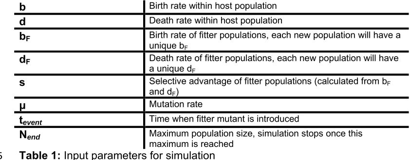
b Birth rate within host population d Death rate within host population
bF Birth rate of fitter populations, each new population will have a
unique bF
dF Death rate of fitter populations, each new population will have
a unique dF
s Selective advantage of fitter populations (calculated from bF and dF)
μ Mutation rate
tevent Time when fitter mutant is introduced
Nend Maximum population size, simulation stops once this maximum is reached
Table 1: Input parameters for simulation 765
766
The simulation algorithm is as follows: 767
768
1. Simulation initialized with 1 cell and set all simulation parameters. 769
2. Choose a random cell, i from the population. 770
3. Draw a random number r~Uniform(0, bmax+dmax), where bmax and dmax
771
are the maximum birth and death rates of all cells in the population. 772
4. Using r, cell i will divide with probability proportional to its birth rate bi
773
and die with probability proportional to its death rate di. If bi+di
774
<bmax+dmax there is a probability that cell i will neither divide nor die. If
775
= 1, ie no cell death then in the above dmax = 0.
776
5. If cell divides, daughter cells acquire new mutations where 777
~Poisson(μ). 778
6. Time is increased by a small increment ( ) , where is an 779
7. Go to step 2 and repeat until population size is Nend. 781
782
The output of the simulation is a list of mutations for each cell in the final 783
population. 784
785
Generating millions of simulations for parameter inference 786
787
A number of simplifications to our simulation scheme were made to improve 788
computationally efficiency when used in our Bayesian inference method, a 789
procedure that requires potentially many millions of individual simulations to 790
be run in order to get accurate inferences. Our ultimate goal was to measure 791
the time subclones emerge and their fitness. These parameters are measured 792
in terms of tumour volume doublings, not in terms of cell division durations (as 793
this is unknown in human tumours). Our approximations allow us to quantify 794
relative fitness of subclones, measured in units of population doubling, from 795
the VAF distribution. The approximations are: 796
797
Approximation 1: We model differential subclone fitness by varying the birth 798
rate only, and setting the deth rate to 0 (e.g. = 1, all lineages survive). This 799
increases simulation speed because a smaller number of time steps are 800
required to reach the same population size and ensures that tumours never 801
die out in our simulations. 802
803
Timing the emergence of subclones depends on the number of mutations that 804
have accumulated in the first cell that gave rise to the subclone. This is the 805
product of the number of divisions and the mutation rate ( × ), or 806
equivalently the number of tumour doublings × the effective mutation rate 807
( × ). Given we measure everything in terms of tumour doublings 808
and the effective mutation rate ( / ) is the only measure available to us from 809
the VAF distribution (from the low frequency 1/f tail), we reduce our search 810
space by fixing = 1 and varying , recognizing that in reality the effective 811
mutation rate is likely to have < 1. 812
813
We do note however that cell death ( < 1) can affect our inferences in two 814
ways. First of all, in the presence of one or more subclones, the low-frequency 815
tail which encodes consists of a combination of two or more 1/f tails. If there 816
are large differences in the value between subclones, then the inference on 817
the effective mutation rate from the gradient of the low-frequency tail may be 818
incorrect. For example, a fitter subclone could arise due to decreased cell 819
death rather than increased proliferation. To quantify this effect, we simulated 820
subclones with differential fitness due to decreased cell death and measured 821
the error on the inferred . Even in cases where the death rate was 822
dramatically different in the subclone compared to the host population 823
( = 1.0 vs = 0.5) the mean error on the estimates of the mutation rate was
824
42% (Supplementary Figure 5), significantly less than the order of magnitude 825
previously measured between cancer type11 and so we conclude that the
826
that we may underestimate the effects of drift, which will be accentuated in 828
tumours with high death rates. 829
830
Approximation 2: We simulate a smaller tumour population size compared to 831
typical tumour sizes at diagnosis, and scale the inferred values a posteriori. 832
We note that the VAF distribution holds no information on the population size 833
(it measures only relative proportions) and furthermore simulating realistic 834
population sizes (in the order of tens or hundreds of billions of cells in human 835
malignancies) is computationally unfeasible. To circumvent this, we generate 836
synthetic datasets that capture the characteristics relevant to measuring the 837
fitness and time subclones emerge, namely the effective mutation rate 838
( ) encoded by the low frequency part of the distribution, the number of 839
mutations in any subclonal cluster and their frequency. Theoretical population 840
genetics is then used to transform these measurements into values of fitness 841
and time (via Equations [2] and [4]), and values are scaled by the realistic 842
population size = 10 . 843
844
Simulation length was required to allow the single cell that gives rise to the 845
subclone sufficient time to accumulate the number of mutations ultimately 846
observed in the empirical datum. In general, we found Nend=103 to be
847
sufficient, except for the breast cancer and AML samples where we used the 848
more conservative Nend=104. In general, Nend=104 is sufficient to be able to
849
measure the range of parameters considered in Figure 1e. 850
851
To appropriately scale the estimates of s requires an estimate of the age of 852
the tumour in terms of tumour doublings. Using Equation [4] with a final 853
population size of , we can calculate as: 854
855
= (( )× )
( ) , [10]
856 857
where is the frequency of the subclone. We assumed a realistic =
858
10 , for generating the posterior distributions in Figures 3 & 4. We also 859
generated posterior distributions for s as a function of , for the AML, 860
breast and lung cancers. For realistically large Nend (>109) the exact choice 861
has minimal effect on our inferred values of s (Supplementary Figure 6). 862
863
To confirm that these assumptions do not invalidate our approach, we 864
generated synthetic datasets with cell death and large final population size 865
(106). We then used our inference method (detailed below) with the 866
simplifying assumptions to infer the parameters used to generate these 867
synthetic tumours. This demonstrated that we were able to accurately recover 868
the input parameters when the simplifications were applied (Figure 2). 869
870 871
Sampling 872
To mimic the process of data generation by high-throughput sequencing we 873
performed various rounds of empirically-motivated sampling of the simulation 874
data. Sequencing data suffers from multiple sources of noise, most 875
true underlying frequencies in the tumour population (both because of the 877
initial limited physical sampling of cells from the tumour for DNA extraction, 878
and then due to the limited read depth of the sequencing). Additionally, it is 879
challenging to discern mutations that are at low frequencies from sequencing 880
errors, and the limited sampling of sequencing assays means that many low 881
frequency mutations are likely not measured at all. Consequently only 882
mutations above a frequency of around 5-10% with 100X sequencing are 883
observable with certainty48. The ability to resolve subclonal structures is thus
884
dependent on the depth of sequencing. 885
886
Our sampling scheme to generate synthetic datasets was as follows. For 887
mutation i with true frequency VAFtrue, the sequence depth Di is Binomially
888
distributed: 889
~ = , =
for a tumour of size N. The sampled read count with the mutant is Binomially 890
distributed with the following parameters: 891
~ = , =
or if over-dispersed sequencing is modelled49,50 we use the Beta-Binomial
892
model, which introduces additional variance to the sampling: 893
~ = , = ,
where is the overdispersion parameter, and = 0 reverts to the Binomial 894
model. Finally, the sequenced VAF for mutation i is given by: 895
=
896
Modelling stem cells 897
Stem cell architecture was modelled with two-compartments: long lived stem 898
cells and short lived non-stem cells. Stem cells divided symmetrically to 899
produce two stem cells with probability and asymmetrically to produce a 900
single stem cell and a single differentiated cell with probability 1 − . 901
Differentiated cells divided n further times before dying. At each division all 902
cells accumulated mutations as described above. We used = 0.1 and n=5. If 903
= 1.0 then the model is equivalent to the above exponential growth model.
904 905
Bayesian Statistical Inference 906
We used Approximate Bayesian Computation (ABC) to infer the evolutionary 907
parameters. We evaluated the accuracy of our inferences using simulated 908
sequencing data where the true underlying evolutionary dynamics was known. 909
The simulation approach to generate synthetic data was taken instead of a 910
purely statistical approach, as the simulation naturally accounts for effects that 911
would be difficult to represent in a pure statistical model (such as the 912
convolution of multiple within subclone mutations at lower frequency ranges). 913
Furthermore, the posterior distribution reported from this method naturally 914
account for uncertainties due to experimental noise and stochastic effects 915
such as Poisson-distributed mutation accumulation and stochastic birth-death 916
processes. For in-depth discussion on these stochastic effects, see the 917
919
As in all Bayesian approaches, the goal of the ABC approach was to produce 920
posterior distributions of parameters that give the degree of confidence that 921
particular parameter values are true, given the data. Given a parameter 922
vector of interest θ and data D, the aim was to compute the posterior 923
distribution ( | ) = ( | ) ( )( ) , where ( ) is the prior distribution on θ and 924
( | ) is the likelihood of the data given θ. In cases where calculating the
925
likelihood is intractable, as was the case here where our model cannot be 926
expressed in terms of well-known and characterized probability distributions, 927
approximate approaches must be sought. The basic idea of these ‘likelihood 928
free’ ABC methods is to compare simulated data, for a given set of parameter 929
values, with observed data using a distance measure. Through multiple 930
comparisons of different input parameter values, we can produce a posterior 931
distribution of parameter values that minimise the distance measure, and in so 932
doing accurately approximate the true posterior. The simplest approach is 933
called the ABC rejection method and the algorithm is as follows51: 934
935
1) Sample candidate parameters θ* from prior distribution π(θ) 936
2) Simulate tumour growth with parameters θ* 937
3) Evaluate distance, δ between simulated data and target data 938
4) If δ<ε reject parameters θ* 939
5) If δ≥ε accept parameters θ* 940
6) Return to 1 941
942
We used an extension of the simple ABC rejection algorithm, called 943
Approximate Bayesian Computation Sequential Monte-Carlo (ABC SMC)22,52. 944
This method achieves higher acceptance rates of candidate simulations and 945
thus makes the algorithm more computationally efficient than the simple 946
rejection ABC. It achieves this increased efficiency by propagating a set of 947
‘particles’ (sample parameter values) through a set of intermediate 948
distributions with strictly decreasing ε until the target εT is reached, using an
949
approach known as sequential importance sampling53. The ABC SMC 950
algorithm also allows for Bayesian model selection to be performed by placing 951
a prior over models and performing inference on the joint space of models 952
and model parameters, (m, θm). In contrast to many applications of ABC that
953
use summary statistics, we use the full data distribution, thus avoiding issues 954
of inconsistent Bayes factors due to loss of information54,55. For further details
955
on the algorithm see references22 and the Supplementary Note on the specific 956
details of our implementation. Bayes factors for all data are shown in 957
Supplementary Tables 4 and 5. We found that the probability of neutrality was 958
significantly correlated with our frequentist based neutrality metrics and that 959
the inferred mutation rates were highly similar (Supplementary Figure 19). 960
961
The clonal structure of the cancer is encoded by the shape of the VAF 962
distribution, we therefore used the Euclidean distance between the two 963
cumulative distributions (simulated and target datasets) for our inference. 964
965
We also refined a simple analytical test in order to rapidly determine what 967
evolutionary parameters of selection lead to an observable deviation of the 968
VAF distribution from that expected under neutrality. Previously, we showed 969
that under neutrality, the distribution of mutations with a frequency greater 970
than f is given by11: 971
972
( ) = − [11]
973 974
We fit a linear model of M(f) against 1/f and used the R2 measure of the 975
explained variance as our measure of the goodness of fit. 976
977
Another approach is to use the shape of the curve described by Equation [5] 978
and test whether our empirical data collapses onto this curve. To implement 979
this approach, here we defined the universal neutrality curve, ( ). Given an 980
appropriate normalization of the data, the mutant allele frequency distribution 981
governed by neutral growth will collapse onto this curve, although we 982
recognize that deviations due to stochastic effects are possible. We can 983
normalize the distribution described by Equation [5] by considering the 984
maximum value of M(f) at f=fmin.
985 986
max ( ( )) = − [12]
987 988
( ) = ( ( )) [13]
989 990
( ) = [14]
991
992
( ) is independent of the mutation rate and the death rate and therefore 993
allows comparison with any dataset. To compare this theoretical distribution 994
against empirical data we used the Kolmogorov distance, Dk, the Euclidean
995
distance between ( ) and the empirical data and the area between ( )
996
and the empirical data. The Kolmogorov distance Dk is the maximum distance
997
between two cumulative distribution functions. Supplementary Figure 1 998
provides a summary of the different metrics. 999
1000
To assess the performance of the 4 classifiers we ran 105 neutral and non-1001
neutral simulations and compared the distribution of the test statistics for 1002
these two cases. Due to the stochastic nature of the model, not all simulations 1003
that include selection will result in subclones at a high enough frequency to be 1004
detected, therefore to accurately assess the performance of our tests we only 1005
included simulations where the fitter subpopulation was within a certain range 1006
(20% and 70% fraction of the final tumour size). All 4 test statistics showed 1007
significantly different distributions between neutral and non-neutral cases 1008
(Supplementary Figure 2). Under the null hypothesis of neutrality and a false 1009
positive rate of 5%, the area between the curves was the test statistics with 1010
the highest power (67%) to detect selection, slightly outperforming the 1011
Kolmogorov distance and Euclidean distance, with the R2 test statistics