Modeling and Analysis of Opportunistic Routing in
Multi-hop Wireless Networks
Amir Darehshoorzadeh
∗, M. Isabel Sanchez
∗†‡and Azzedine Boukerche
∗∗PARADISE Research Laboratory - School of Electrical Engineering and Computer Science
University of Ottawa, Canada
†IMDEA Networks Institute, Spain
‡Departamento de Ingenieria Telematica, University Carlos III, Madrid, Spain
Email: [email protected], [email protected], [email protected]
Abstract—Opportunistic Routing (OR) takes advantage of the broadcast nature of the wireless medium to increase reliability in communications. Instead of selecting one node as the next-hop forwarder, OR selects a set of candidates to forward the packet. In this way, if one of them does not receive the packet from the source, another candidate will be able to do it; this avoids the need for a re-transmission from the source. To increase the successful delivery ratio, we can increase the size of the candidate set or the number of re-transmissions, but, we must take into account the impact on the use of the network resources. In this paper, we propose a Markov chain as a general model for OR that can be applied to any kind of network topology and any candidate selection algorithm without any constraint. The only input parameters needed are: i) the candidate list of each node; ii) the link delivery probability between nodes; and,iii)the maximum number of re-transmissions in each node. Taking this data into account, our model allows for the evaluation of the performance of different candidate selection algorithms according to different metrics, such as the expected number of transmissions (ExNT), which is one of the most relevant metrics in OR. Our model also enables an evaluation of the influence of the number of candidates, its relation to the number of re-transmissions and how these two parameters together contribute to the successful delivery of data packets.
I. INTRODUCTION
Traditional routing in wireless networks designates just one node as the next-hop forwarder to a given destination. If the selected next-hop does not receive the packet, the source must re-transmit it. Therefore, in traditional routing protocols, all packets travel through a pre-defined path [1], [2]. A link breakage over the selected path forces the finding and establishing of a new path and the re-transmission of data with the subsequent costs in terms of time and bandwidth.
Opportunistic Routing (OR) [3] has been a hot research topic for a few years now. The basic idea behind OR is that it selects the next-hop forwarder on-the-fly, as the packet progresses through the network by taking advantage of the broadcast nature of the wireless medium. In other words, instead of establishing a single next-hop to forward the
packets, OR selects an ordered set of nodes (candidate set)
as the potential next-hop forwarders. The source of a data transmission includes its candidate set in the header of every data packet and broadcasts it. Each of the candidates which receives the packet can act as the next-hop forwarder. Note that each candidate has a priority level which determines the
preference for that candidate over the other ones to act as the next-hop forwarder. The priority assignment for candidates follows certain criteria: distance to the destination, hop count or battery constraints [4]. In this way, only the most suitable candidate among those which have received the packet will forward it while the rest of the candidates will discard it.
OR introduces different challenges to the design and eval-uation of OR protocols, for instance, the selection of the candidates for the next transmission and the coordination among them to select which one will actually forward the packet. The main aim of an OR protocol is to reduce the expected number of transmissions (ExNT) from source to destination while increasing the probability of reaching the destination.
each node in the case that the packet does not reach any of the candidates. Our model allows to evaluate the impact of a limited number of re-transmissions, and assess whether the use of OR and several candidates can compensate the need for retries. As a result, the use of our model can provide the guidelines to other researchers to evaluate the performance of different candidate selection algorithms, and to investigate the influence of the number of candidates, how it relates to the number of re-transmissions and how these two parameters together contribute to the successful delivery of data packets. The remainder of this paper is organized as follows: in Section II we present the related work available in the literature which also covers existing analytical models in OR. Section III introduces the Markov model proposed to analyze the performance of OR. This analytical model is validated with a linear topology presented as a case study in Section IV, which illustrates some graphs and results that support our model. Finally, Section V concludes the paper.
II. RELATED WORK
Markov processes have been extensively used to model a huge variety of stochastic processes, from chemistry to economics, not limited to the field of network communica-tions. Although they have been applied to queuing theory and wireless networks, to our knowledge, only [11], [12] has applied these processes to Opportunistic Routing (OR). In [11], it is assumed that the packets could be transmitted an infinite times until it reaches to the destination. the contrary, we limit the number of times that a node can re-transmit a packet. There are several reasons to justify this decision. First of all, if the link conditions are not stable enough, every node may need several re-transmissions to successfully deliver the packet, increasing the contention and the delay. Moreover, the strength of OR resides in the use of several candidates to avoid re-transmitting. In addition, after some time, the packet information may not be meaningful. Secondly, as we show in Section IV, a low number of re-transmissions can considerably improve the network performance; therefore, it is not necessary to allow an infinite number of retries.
Another approach [13] is based on the claim that trans-mitting packets at different rates may increase the throughput of OR, but the communication range associated with different rates must also be taken into account. [14] optimizes candidate selection by minimizing the distance towards the destination, according to a given routing metric. Specifically, the average number of transmissions is selected as the routing metric. The authors proposed two algorithms for finding the optimum can-didate list, considering the trade-off between the probability of reaching the destination and the number of transmissions.
In [15] arandom walk model in a Markov chain is used to
analyze the end-to-end transmission cost of different routing mechanisms, being OR among them. Like our model, [15] also focuses on the expected number of transmission as the metric to evaluate performance, as it is the most relevant in OR. However, their model assumes that a packet can be indefinitely
. . . N
1 2
x= D N−1
3
D
d s
Fig. 1. Linear topology
re-transmitted until it finally reaches the destination, and the system is solved using a different method.
The analytical model for OR based on Markov chains that we propose allows to evaluate the performance of OR in a given network scheme in a simple yet effective way. To the best of our knowledge, our model is the first one to consider a finite number of re-transmissions in the case where none of the next-hop nodes receive the packet. At the same time, our model provides a very intuitive analysis and allow for evaluating the impact of candidate list size as well as number of re-transmissions in any network topology.
III. MARKOVMODEL
In this section, we introduce our proposal to model Op-portunistic Routing (OR) by a Discrete Time Markov Chain (DTMC). As we have mentioned in Section II, the research on OR topics has been extensively supported by simulation, it has not been so commonly supported by analytical models.
We can establish an analogy between a Markov chain and OR. Assuming perfect coordination between candidates at each packet transmission, only one candidate will forward the packet and the transmission will arrive at the next-hop following a certain probability. There are some proposals in the literature, such as three-way handshaking or RTS-CTS coordination [16], which can provide perfect coordination in OR. However, the focus of this work is the DTMC modeling to be applied to OR, so, to simplify the initial assessment, the coordination between candidates is left out of scope. In addition, for a candidate to receive a packet and to forward it, the source of the packet is not relevant. In the same way, in a Markov chain, at each step the system can be only in one state and the future states depend only on the current state, but not on the past ones. Furthermore, in OR, each candidate can receive a packet from the previous node with a certain probability and the transmission of the packet will stop when it reaches the destination or the packet is dropped by any nodes. As we can see, the properties of OR are very similar to a Markov chain with absorbing states; which are in this case the equivalent to the delivery or dropping of the packet. In the following sections, we show how an OR protocol can be modeled by a Markov chain.
A. Markov model for OR and linear topology
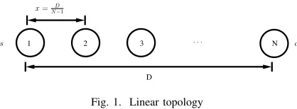
Consider a linear network topology shown in Figure 1
with N nodes numbered from 1 to N and equally spaced
x meters, with s and d as the source and the destination,
respectively. The candidate set fromsto reach destinationd, is
Cs
.
. . .
.
. . .
.
. . .
.
. . .
.
. . . .
. . .
.
. . .
.
. . .
.
. . .
.
. . .
.
. . .
1
Fail
N+1,K+1
p1
p2 p10
2, 0
1, K 2, K
2, 1
p3
p2
1, 0
1, 1
p1
p1
p2
p3
p3
p3
p3
p3
p3
N-1, 0
N-1, K
p30
N-1, 1
p30
N,0 Dest
1
p30
p30
Fig. 2. Markov Model
c1 > c2 > · · · > cncand. That is, candidatecj will forward the packet if none of the higher priority candidates (ci, i < j) receives the packet.
The source broadcasts a packet that will be forwarded by the highest priority candidate which received the packet, while the lower priority candidates will discard it. In other words, we have assumed that there is a perfect coordination between candidates. If the transmitted packet does not reach any of
candidates, a node can re-transmit it at mostReT x=Ktimes.
This process continues until the packet reaches the destination or until it is discarded by one of the intermediate nodes after
K failed re-transmissions.
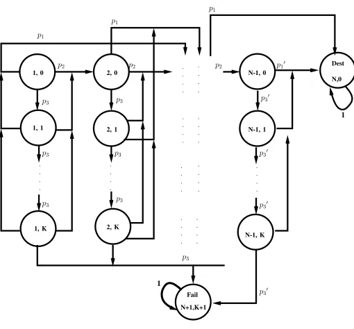
We can model the OR linear topology with a Discrete Time Markov Chain (DTMC) like the one depicted in Figure 2. For the sake of clarity, we have assumed that the number of
candidates in each node is ncand = 2. Each state in our
model represents a node and the number of re-transmissions being performed by that node to make the packet progress towards the destination. The state transitions in our Markov chain reflect how the packet progresses through the network. If the packet progresses towards the destination, it moves to the right in the Markov chain. On the contrary, if the packet needs to be re-transmitted, it will be moved to its respective downward state. Note that the obtained Markov model has two
absorbing states (see Figure 2): state Destcorresponds to the
successful delivery of the packet to the destination and Fail
state corresponds to a dropped packet because the node has
transmitted the packetK times.
Each state in our model is labeled with<ID, re-tx>where
IDis the node identification and re-txis the number of times
that the packet is being re-transmitted by that node. Recall that
each node is allowed to re-transmit a packet at most ReTx=K.
The first row of states, in the model presented in Figure 2,
corresponds to the case in which nodes can deliver the packet to one of the candidates in the first transmission. The second row of states, (<ID, 1 >, ID ∈ {1,2, . . . N−1}) signifies that the first transmission failed and that the node needs to re-transmit the packet. This sequence of re-transmissions
con-tinues until a node has completed ReTx=K re-transmissions
(as shown in the subsequent rows), and then the packet is
dropped: i.e., it reaches theFailabsorbing state. If every node
can deliver the packet to one of its candidates, the packet will
eventually reach the other absorbing state (i.e. Dest state);
this represents the successful delivery of the packet to the destination node. Note that there are no transitions between the states in the second and the lower rows (all rows except the first one), because when a re-transmission reaches one of the candidates, that candidate will continue forwarding the packet in its first transmission attempt.
To build up the transition probability matrix, we need to obtain the transition probabilities between states. Let us
assume thatp(x)is the probability of reaching a node located
at a distancex. As we mentioned above, with perfect
coordi-nation between candidates, the lowest priority candidate will forward the packet if the highest priority one does not receive the packet. Therefore, the probabilities corresponding to each transition between each state can be obtained as follows:
p1=p(2x)
p2 =p(x)×(1−p1)
p3= 1−(p1+p2)
p01=p(x)
p03= 1−p
0
1
(1)
wherep1 andp2 are the probabilities that the highest priority
candidate (c1) and the second highest priority candidate (c2)
will forward the packet, respectively. Note that each node will
re-transmit the packet, if none of the candidates (c1 andc2)
receives the packet. This has been shown asp3 in Equation 1.
The probabilities p01 andp03 are the probabilities of reaching the destination in the last hop or having to re-transmit the packet, respectively.
Note that the Markov model presented in Figure 2 applies to a linear topology like the one shown in Figure 1 with
ncand=2candidates and ReTx=K. In the next section, we will
show how we can apply our proposed model to any kind of network topology; this can be done regardless of the number of candidates and the candidate selection algorithm.
B. How to generalize and to solve the OR Markov chain
As we have showed in the previous section, there is a great similarity between OR and a DTMC; and, we have shown
how we can model an OR linear topology with ncand = 2
candidates using a Markov chain. We can obtain a similar
Markov chain model forncand≥3. Furthermore, the model
selection algorithm can be applied on the network topology to find the candidate set from source to the destination, and the candidate set is given to the model as one of its necessary inputs. As we can see, the obtained model can be applied with any number of candidates and candidate selection algorithms. To solve the proposed Markov chain the first thing needed to be defined is the transition probability matrix and the dimension needed to build it. According to the definition
of each state in Section III-A, in a network with N nodes
and a maximum number of re-transmissions ReTx=K, the
number of transient states in our model is equal to (N−1)×
(K+ 1), in addition to the two absorbing states. Therefore,
the transition probability matrix has a dimension equal to
[(N−1)×(K+ 1) + 2]×[(N−1)×(K+ 1) + 2].
Recall that, each state in our model is labeled with <ID,
re-tx>. Each transient state (all states except Dest andFail) is mapped to an index in the transition probability matrix according to the node’s ID and the number of re-transmissions
so that index=ID+ (re−tx)×(N-1). For the absorbing states
we consider the state index = (N −1) ×(K + 1) + 1
as the state where the packet is dropped (Fail) and state
index = (N −1)×(K+ 1) + 2 as the destination state
(Dest).
The formal definition of the transition probabilities of our model is completed by the set of equations in 3, in which the transition probabilities between all states are obtained. Note that ci(l), l ∈ {1,2, . . . , ncand}, in Equation 3, is
the candidate of node i with priority l. The first
probabil-ity in Equation 3 is the probabilprobabil-ity of reaching the state < ci(1),0 > from state < i, k > (i ∈ {1,2, . . . , N −1} and k ∈ {0,1, . . . , K}); and; this is equal to the probability
of reaching the candidate ci(1) from nodei. The probability
of reaching the other candidates, but not the highest priority one, is shown in the second probability in Equation 3. The probability of performing a re-transmission for each state can be obtained by the third probability in Equation 3. Finally, the probability of remaining in each state with the exception of
the Dest and Fail is equal to0 (see the forth probability in
Equation 3).
For our convenience, P can be expressed in its canonical
form as: P = Q R 0 I (4)
whereQ(N−1)(K+1)×(N−1)(K+1)contains the transition prob-abilities between transient states,R(N−1)(K+1)×2contains the transition probabilities from transient states to the absorbing
states and I2×2denotes an identity matrix.
In order to build up the transition probability matrix, all we need is the candidate set of each node and the maximum
number of re-transmissionsK. We can then find out different
metrics such as the probability of a successful transmission from a source to a destination using OR, the probability of a failed transmission and the expected number of transmissions needed to reach the destination. In the following text we
explain how we can derive this information from matrix P.
The transition matrix P shows the probability for going
pi,ji0,j0=
p(i, ci(1)),
1≤i≤N−1, i0=ci(1)
0≤j≤ReT x, j0= 0
p(i, ci(k)) k−1
Y
l=1
(1−p(i, ci(l))),
1≤i≤N−1, i0=ci(k)
0≤j≤ReT x, j0= 0
k= 2, ..., ncand
1−
ncand
X
l=1
pi,jc i(l),0,
1≤i≤N−1, i0=i∪(N+ 1)
0≤j≤ReT x, j0=j+ 1
1,
i=i0=Nandj=j0= 0
or
i=i0= (N+ 1)andj=j0= (K+ 1)
(3)
from one state to every other state in one step. However, the destination may not be reachable from the source in only one step. To obtain the probability of reaching the destination from the source node, we need to find the probability of reaching
the destination in h steps. This probability is given by the
powers of P. Equation 5 shows the h-th power of P shows
the probability of going from state i to other states after h
steps.
Ph=
Qh (I+Q+...+Qh−1)×R
0 I
(5)
In the stationary stateh→ ∞,(I+Q+Q2...+Qh−1) =
(I−Q)−1. The matrix N = (I−Q)−1 is known as the
fundamental matrix of the Markov process. Note that N ×
R gives us the probability of being absorbed in every other
transient state. Taking into account that we only consider the path from the source to the destination, the initial distribution of the states in our system is given by:
v=
1 0 · · · 0
(6)
therefore, after hsteps the probability of reaching any other
state from the source is:v×Ph, which corresponds to the first
row ofPh. Particularly,p
1,1inN×Rpresents the probability of dropping the packet which is transmitted by the source; and, the value ofp1,2is the probability of a successful transmission from source to the destination.
Another very important metric in OR that can be easily derived from our Markov model is the expected number of
transmissions from source to the destination. Let X be the
random variable equal to the number of transitions from state iuntil the destination absorption state (Deststate). It is clear that the probability of transitioning from a transient stateito a transient statejin exactlyh−1steps is theqi,jentry ofQh−1
in matrix Ph−1. Therefore, the probability of transitioning
from a non-absorbing state i to the absorbing state j, in h
steps, can be obtained from Equation 7.
S A B 0.7 D 0.1
0.7 0.7
0.2
Fig. 3. Example of a topology
Note thatQh−1×Ris a matrix with dimensions(N−1)(k+
1)×2. The expected value of X is the expected number of
transmissions, which can be derived from Equation 8, where matrices are divided element by element.
E[X] =
P∞
h=1(h×p[X =h]) p[X= 1] +p[x= 2] +. . . =
1×R+ 2Q×R+ 3Q2×R+ 4Q3×R+. . .
R+Q×R+Q2×R+Q3×R+. . . =
(I−Q)−2×R
(I−Q)−1×R =
N2×R
N×R
(8)
C. An example of OR Markov model
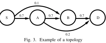
We close the description of our Markov model by providing a simple example to show how we can use our model to evaluate the performance of a network using OR. To do so, we consider a network topology with four nodes in Figure 3. The numbers on each link represent the successful link delivery
probability. Assume that each node can select at most 2
candidates and that the maximum number of re-transmissions
in each node is equal to K = 1. The candidate set for node
S to reach the destination DisCD
S ={B, A}; hereB is the
highest priority candidate. Furthermore, the candidate set for
A to the destination isCAD={D, B}.
This topology and the candidate set in each node lead us to the Markov chain shown in Figure 4(a). For the sake of clarity, we have included in Figure 4(a) the index corresponding to every state in small round ovals next to each of state. These indexes are assigned also due to the positioning in the matrix. In our example, the transition probability from the source to its second candidate (nodeA) is equal top1= 0.7×(1−0.1) =
0.63. However, the source can reach its first candidate with a
probability of 0.1. The source has to once again re-transmit
the packet in case none of the candidates received the original
transmission; it does so with probability p3= 0.27.
By building the matrixPand by applying the(I−Q)−1×R
and Equation 8, we can easily obtain the probability of reach-ing the destination and the expected number of transmissions
that use OR to reach the destination D. We can see that the
probability of reaching the destination state from the source is
0.81and the the ExNT from source to the destination is3.17.
Note that OR with only one candidate is a traditional routing which selects the shortest path from source to the destination. Our model can also be applied to traditional routing. Applying
our model to traditional routing with pathS−A−B−D, as
shown in Figure 4(b), can result in a probability of reaching
the destination equal to0.75with3.69as the expected number
of transmissions needed to reach the destination. As we can
see, OR outperforms traditional routing in terms of successful delivery for reaching the destination with less ExNT.
IV. EXPERIMENTAL ANALYSIS AND VALIDATION
In this section, we show how our model can be used to evaluate the performance of OR in different scenarios. Note that, as we have mentioned in Section III, our Markov model can be applied on any kind of network topology and the candidate selection algorithm. The only ingredients needed in our model are the following: the candidate sets, CiD ={ci(1), ci(2), . . . , ci(ncand)}; the delivery probability of reaching the candidates; and, the maximum number of
re-transmissions,K, which is allowed in each node.
We have used the shadowing model with parameters β =
2.7 as the packet loss and σdB = 6.0 for standard deviation
value in our numerical analysis (see [11] for more informa-tion). As the threshold for the probability to accept a link as an
existing link between two nodes we have usedmin.dp= 0.1.
That is, if the link probability between two nodes is greater
than0.1, we consider that link to be link in the network.
A. Numerical results
In this section, we show the numerical results obtained by applying our model on a linear topology. To show the effect of a different number of re-transmissions and candidates, we have used two different scenarios.
Recall that our Markov model can is applied on any kind of network topology and the candidate selection algorithm. Therefore, we have used a linear topology to enact a simple scenario to illustrate our results. We choose ExOR [3] to select the candidates in our experiments; this is because ExOR is a simple and the most well-known candidate selection algorithm.
We have considered a linear topology with N = 20 nodes
placed at a distance of x = 100 m (see Figure 1). Nodes
vs= 1andvd= 20are considered as source and destination,
respectively. In the following text, the notationORk
mrefers to
OR withReT x=kandncand=mas the maximum number
of candidates for each node. When we measure the effect of these parameters (re-transmissions or number of candidates), the measured parameter is not shown in the notation.
1) The effect of a different number of re-transmissions in
OR: For our first experiment, we have set the maximum
number of candidates in each node as equal to2(ncan= 2).
One of the important measurements in OR is the probability of reaching the destination for a different number of re-transmissions. Figure 5 depicts the results for the probability
of reaching the destination (see state Dest in Figure 2), by
varying number of re-transmissions for OR with ncand=2
(OR2) and uni-path routing. In our comparison, we have added the results of traditional routing, which uses the ETX [17] of each link to find the shortest path from the source to the destination (see legend Uni-path in Figure 5). As we can see in Figure 5, allowing more re-transmissions results in a higher
probability of arriving at the destination state; and, after 4
or 5 re-transmissions for OR2 and uni-path, the probability
0.63
S,1 A,1 B,1
Fail
5 4
7
1 2 3
0.3
0.3 0.27
0.1
0.24 0.27
0.56
0.2
0.7
0.24
6
8
D,0 B,0
A,0 S,0
(a) Markov model of OR in Figure 3
0.7 0.7 0.7
0.3 0.3
S,1 A,1 B,1
Fail
1 2 3 8
6 5
4
7
S,0 A,0 B,0 D,0
0.3 0.3
0.3
0.3
(b) Markov model of traditional routing in Figure 3 Fig. 4. Comparison of Markov chains for traditional and OR for the same network topology
0 1 2 3 4 5 6 7 8 9 10
0 0.1 0.2 0.3 0.4 0.5 0.6 0.7 0.8 0.9 1
OR2
Number of re-transmissions
Probability
of
success
β=2.7,min.dp=0.1,σdB=6.0,N=20
Uni-path
Fig. 5. Probability of success vs number of ReTx for N=20
14 16 18
20
22 24 26 28 30
Number of re-transmissions OR2
β=2.7,min.dp=0.1,σdB=6.0,N=20
Expected
number
of
transmissions
Uni-path
1 2 3 4 5 6 7 8 9 10
0
Fig. 6. Expected number of Transmissions vs Number of ReTx for N=20
10 12 14 16 18 20 22 24 26 28 30 32 34 36 38 40 0
0.02 0.04 0.06 0.08 0.1 0.12 0.14 0.16 0.18 0.2
Uni-path1
Uni-path20
OR1 2
OR20 2
β=2.7,min.dp=0.1,σdB=6.0,N=20, ncand=2
Number of transmissions
Probability
of
reaching
the
destination
Fig. 7. Probability of number of transmissions, N=20, ncand=2.
with a number of candidates as small as 2, can increase the
probability of reaching the destination compared to traditional routing. This comes from the opportunistic use of a set of nodes, instead of only one, which can act as the next-hop forwarder; this increases the chances to reach the destination. This conclusion has been obtained in [18] where the effect of the number of candidates in OR was investigated.
Another important and well-know metric in OR is the expected number of transmissions (ExNT) from source to
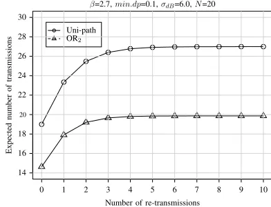
the destination. Figure 6 shows the expected number of transmissions for the linear topology under study, varying the
number of re-transmissions (ReTx=0,1, . . . ,10). As a first
observation, in Figure 6, we can see that OR with only 2
candidates (OR2) outperforms the uni-path routing in terms of
the expected number of transmissions (ExNT). Furthermore, allowing more re-transmissions in each node increases the expected number of transmissions (ExNT), but after a certain number of re-transmissions the ExNT needed to reach the
destination remains stable. For instance, in the case of OR2,
after ReT x = 4, the ExNT remains the same; on the other
hand, for the traditional routing, the ExNT stops increasing
after ReT x= 6. This comes from the fact that having more
re-transmissions increases reliability; thus, the probability of a packet reaching the destination is increased. Therefore, the
probability of being in stateDestand reaching the destination
increases, by allowing a higher number of re-transmissions; this also increases the ExNT. However, increasing the number
of re-transmissions over 4 for OR and over 6 for uni-path
is not useful; it does not translate into gain in terms of the ExNT nor does it increase reliability. Considering the obtained results in Figure 5, we can see the difference between the probabilities of reaching the destination when the number of
is about1%; however, as we can see in Figure 6, OR can reach
the destination in26%less number of transmissions than
uni-path routing.
Figure 7 shows a more detailed comparison of OR and uni-path routing by using our proposed Markov model to find the probability of the number of transmissions needed for a linear
topology with N=20 nodes. The number of re-transmissions
is set to 1 (OR1 and Uni-Path1); and, we also included the
results for both routing mechanisms when the number of
re-transmissions is big enough (ReTx=20) to satisfy the fact that
the probability of being absorbed by the destination state is
equal to 1 (legends OR20 and Uni-path20 in Figure 7).
First of all, Figure 7 confirms that by using OR, we can end at the destination state with a higher probability and a smaller number of transmissions. In other words, the obtained results in a network reveal that by using OR in the considered scenario results in a higher packet delivery ratio to the destination while less transmissions are needed than uni-path routing requires. As we can see, when there are enough re-transmissions to
ensure that we end at the destination state (ReTx=20), by using
OR (OR20),10%of the packets are delivered to the destination
with17transmissions; on the other hand, the same percentage
of packets (10%) reach the destination with24transmissions,
in the case where uni-path routing (Uni-path20) is used. The
same situation will happen when we have a limited number
of re-transmissions; ReTx=1. That is7%of packets reach the
destination with17transmissions, while in the uni-path routing
about 4%of the packets are delivered to the destination with
23transmissions. Note that the sum of every value obtained in
each curve is equal to the corresponding point in Figure 5; e.g,
the sum of the obtained values in the case ofOR12 is equal to
0.4, which is the same value at ReTx=1for OR in Figure 5.
2) The effect of a different number of candidates in OR:
As we have mentioned before, two of the main parameters which have an effect on the performance of an OR protocol are the number of re-transmissions of a packet in each node and the number of candidates. In this section we use our Markov model to investigate the effect of a different number of candidates on the performance of an OR approach. We
have used the same linear topology, in this case with N= 40
nodes in the network, and a varying number of candidates ncand=1,2,3, . . . ,5.
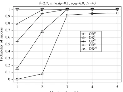
Figure 8 depicts the probability of reaching the destination with a different number of candidates (ncand = 1,2, . . . ,5) for different a number of re-transmissions; ReTx=0,1,2,3,20
(see legends in Figure 8). Recall that OR with ncand = 1
is equal to the uni-path routing approach. Therefore, the first point in Figure 8 represents uni-path or traditional routing for a different number of re-transmissions, while the other points correspond to OR.
The first observation for Figure 8 is the more candidates that are selected, the higher the probability of reaching the destination becomes. In addition, by having the same number of candidates and by increasing the number of re-transmissions (ReTx), the success probability is also considerably increased,
at least for a number of candidates; ncan< 3. Considering
the results with no re-transmissions (OR0), we can see that in
order to increase the probability of success we need to include more candidates in the set. Note that with three candidates, the chances of reaching the destination are significantly higher
than with one and two. The success probability in the case of3
candidates with ReTx=2is approximately0.98. The difference
with the probability in the case of2candidates and ReTx=2,3
is very small; all probabilities are over0.9. However, by having more candidates duplicated packets may be caused if there is imperfect coordination among the candidates.
Figure 9 depicts the ExNT for a different number of candidates with varying numbers of re-transmissions. As in Figure 5, we have added the results of uni-path routing. We can see that with any number of candidates OR outperforms the uni-path routing in terms of ExNT. Furthermore, the ExNT decreases as the number of candidates in the set increases. This is due to the greater chance of delivering the packet to the destination when there are more candidates; any candidate may receive the packet and forward it eventually; within a lower number of transmissions. As we can see, the increase
in terms of ExNT for uni-path stops after approximately9
re-transmissions. However, in the case of 2 candidates (OR2),
the ExNT does not change after 3 re-transmissions. This
can also be explained by the results in Figure 8 that show the probability of success with a different number of re-transmissions when using different number of candidates in
the set. When the number of re-transmissions is ReTx≥ 3,
the transmissions always end up in the absorbing state of the destination. Therefore, allowing more re-transmissions when the probability of being absorbed by the destination is close to
1 does not increase the ExNT from source to the destination.
Figure 10 shows additional results for the probability of
transmissions for N=40 nodes with a different number of
candidates. In the case of 2 candidates, we have shown the
results for a different number of re-transmissions (ReTx=0,1).
Note thatanyin the legends in Figure 10 shows any number
of re-transmissions. This is because in the case of a large
number of candidates, e.g 3, the results for any number of
re-transmissions are the same.
The probabilities for transmissions in Figure 10 for a differ-ent number of candidates show that by using a greater number of candidates in OR, a smaller number of transmissions is
caused. For instance, in the case of ORany5 , 24% of the
packets are delivered to the destination with14transmissions;
however for this number of transmissions when there are
4 candidates (ORany4 ), about 20% of the packets reach the
destination. Comparing the obtained results of OR0
2 and OR12,
we can see that with ReTx=0, about4%of the packets reach
the destination with 16 transmissions; on the other hand,
for ReTx=1, about 8% of the packets are delivered to the
destination with the same number of transmissions (16).
V. CONCLUSION
1 2 3 4 5 0
0.1 0.2 0.3 0.4 0.5 0.6 0.7 0.8 0.9 1
OR0 OR1
OR3
OR20
β=2.7,min.dp=0.1,σdB=6.0,N=40
Number of candidates
Probability
of
success
OR2
Fig. 8. Probability of success varying the number of candidates for N=40
0 1 2 3 4 5 6 7 8 9 10
12 16 20 24 28 32
Uni-path OR2 OR3 OR4 OR5
β=2.7,min.dp=0.1,σdB=6.0,N=40
Number of re-transmissions
Expected
number
of
transmissions
Fig. 9. Expected number of transmissions varying the number of re-transmissions for N=40
5 7 9 11 13 15 17 19 21 23 25 27 29
0 0.04 0.08 0.12 0.16 0.2 0.24 0.28
OR0 2 OR1 2 ORany
3 ORany
4 ORany
5
β=2.7,min.dp=0.1,σdB=6,N=40
Number of transmissions
Probability
Fig. 10. Probability N=40, ReTx=5 different candidates
network performance. Most of the existing research focuses on this aspect from a simulation-based approach.
In this paper, we have proposed a Discrete Time Markov chain (DTMC) that enables the performance of OR to be evaluated in a very simple, fast and effective way. Our model is valid for any network topology and any candidate selection algorithm and can be evaluated through it. In addition, our model accounts the number of re-transmissions in the case none of the candidates receive the packet. To the best of our knowledge, our model is the first one that takes this issue into account. The proposed model takes into account the number of re-transmissions and is valid for any number of candidates, so both parameters can be easily evaluated when designing an OR protocol. As a result, the use of our model can provide guidelines to other researchers for evaluating the influence of the number of candidates, how this relates to the number of re-transmissions and how these two parameters together contribute to the successful delivery of the data packets.
ACKNOWLEDGMENT
This work has been partially supported by Canada Research Chairs program, NSERC Discovery, NSERC DIVA Strategic Networks and the European Community through the CROWD project (FP7-ICT-318115).
REFERENCES
[1] A. Boukerche, B. Turgut, N. Aydin, M. Ahmad, L. B¨ol¨oni, and D. Turgut, “Routing protocols in ad hoc networks: a survey,”Computer Networks, vol. 55, no. 13, pp. 3032–3080, September 2011.
[2] A. Boukerche, “Performance evaluation of routing protocols for ad hoc wireless networks,”Mobile Networks and Applications, vol. 9, no. 4, pp. 333–342, 2004.
[3] S. Biswas and R. Morris, “Opportunistic routing in multi-hop wireless networks,”ACM SIGCOMM Computer Communication Review, vol. 34, no. 1, pp. 69–74, 2004.
[4] X. Mao, X.-Y. Li, W.-Z. Song, P. Xu, and K. Moaveni-Nejad, “Energy efficient opportunistic routing in wireless networks,” inProceedings of MSWIM ’09. New York, NY, USA: ACM, 2009, pp. 253–260. [5] C.-J. Hsu and H.-I. Liu, “Route selection for opportunistic routing in
multi-channel scenario,” inICC 2013, 2013, pp. 6294–6299.
[6] Z. Yang, K. Zeng, and W. Lou, “FSA: A Fast Coordination Scheme for Opportunistic Routing,” inICC 2009. IEEE, Jun. 2009, pp. 1–5. [7] Y. Li, W. Chen, and Z.-L. Zhang, “Optimal forwarder list selection
in opportunistic routing,” inMobile Adhoc and Sensor Systems, 2009. MASS ’09. IEEE 6th International Conference on, 2009, pp. 670–675. [8] H. Dubois-Ferri´ere, M. Grossglauser, and M. Vetterli, “Valuable detours:
Least-cost anypath routing,” Networking, IEEE/ACM Transactions on, vol. 19, no. 2, pp. 333 –346, april 2011.
[9] B. Sen, X. Zhao, L. Libman, and S. Jha, “Relay-aided high-throughput path selection in multi-rate wireless mesh networks,” inProceedings of MSWiM ’12. New York, NY, USA: ACM, 2012, pp. 223–228. [10] M. F. Neuts, Matrix-Geometric Solutions in Stochastic Models: an
Algorithmic Approach. Dover Publications Inc., 1981.
[11] A. Darehshoorzadeh, L. Cerd`a-Alabern, and V. Pla, “Modeling and comparison of candidate selection algorithms in opportunistic routing,”
Computer Networks, vol. 55, no. 13, pp. 2886 – 2898, 2011. [12] L. Cerd`a-Alabern, V. Pla, and A. Darehshoorzadeh, “On the performance
modeling of opportunistic routing,” inMobiOpp ’10. New York, NY, USA: ACM, 2010, pp. 15–21.
[13] K. Zeng, W. Lou, and H. Zhai, “On end-to-end throughput of oppor-tunistic routing in multirate and multihop wireless networks,” inIEEE INFOCOM, 2008, pp. 816–824.
[14] A. Cacciapuoti, M. Caleffi, and L. Paura, “Optimal constrained candidate selection for opportunistic routing,” inIEEE GLOBECOM, Dec. 2010, pp. 1–5.
[15] Y. Li and Z.-L. Zhang, “Random walks on digraphs: a theoretical framework for estimating transmission costs in wireless routing,” in
INFOCOM’10. IEEE Press, 2010, pp. 2775–2783.
[16] A. Darehshoorzadeh, L. Cerd`a-Alabern, and V. Pla, “Opportunistic rout-ing in wireless mesh networks,” inRouting in Opportunistic Networks. Springer New York, 2013, pp. 289–330.
[17] D. S. J. De Couto, D. Aguayo, J. Bicket, and R. Morris, “A high-throughput path metric for multi-hop wireless routing,” Wireless Net-works, vol. 11, no. 4, pp. 419–434, 2005.