Dynamic Scheduling of a Semiconductor Production
1Line Based on Composite Rule Set
2Yumin Ma1, Fei Qiao1, Fu Zhao2,3, John W.Sutherland3
3
1 School of Electronical & Information Engineering, Tongji University, Shanghai, 201804, China;
4
[email protected] (Y.M. Ma), [email protected](F. Qiao) 5
2 School of Mechanical Engineering, Purdue University, West Lafayette, IN 47907, USA;
6
[email protected](F.Zhao) 7
3 Division of Environmental and Ecological Engineering, Purdue University, West Lafayette, IN 47907, USA;
8
[email protected] (J.W.Sutherland) 9
* Correspondence: [email protected]; Tel.: +86-216-958-8911 10
11 12
Abstract: Various factors and constraints should be considered when developing a manufacturing 13
production schedule, and such a schedule is often based on rules. This paper develops a composite 14
dispatching rule based on heuristic rules that comprehensively consider various factors in a 15
semiconductor production line. The composite rule is obtained by exploring various states of a 16
semiconductor production line (machine status, queue size, etc.), where such indicators as 17
makespan and equipment efficiency are used to judge performance. A model of the response 18
surface, as a function of key variables, is then developed to find the optimized parameters of a 19
composite rule for various production states. Further, dynamic scheduling of semiconductor 20
manufacturing is studied based on support vector regression (SVR). This approach dynamically 21
obtains a composite dispatching rule (i.e. parameters of the composite dispatching rule) that can be 22
used to optimize production performance according to real-time production line state. Following 23
optimization, the proposed dynamic scheduling approach is tested in a real semiconductor 24
production line to validate the effectiveness of the proposed composite rule set. 25
26
Keywords: Dynamic Scheduling; Semiconductor Manufacturing; Composite Rule Set; Support Vector
27
Regression (SVR) 28
29
1. Introduction 30
A semiconductor manufacturing system is a dynamic system that is subject to various 31
uncertainties (e.g., machine failures, arrival of new urgent jobs, and the modification of job due 32
times). When unexpected events occur, a previously “optimal” schedule may no longer be optimal, 33
and can even become infeasible. Scheduling in response to real-time events has been defined as 34
“dynamic scheduling”[1]. 35
Dynamic scheduling of manufacturing systems is often rule based, with a given rule selected 36
based on the needs of the production environment [2]. Some researchers have been studying 37
dynamic scheduling based on a machine learning approach. With this approach, a system acquires 38
scheduling knowledge through training with optimized scheduling samples. This knowledge is then 39
applied to obtain scheduling rules which may be utilized to obtain a feasible real-time schedule. For 40
example, Shiue et al. [3] proposed a self-organizing map-based multiple scheduling rule selection 41
mechanism. Tsai et al. [4] put forward a radio frequency identification (RFID)-based real-time 42
scheduling system for an automated semiconductor manufacturing plant, which selected features 43
for training samples and established a dynamic scheduling model based on a support vector 44
machine (SVM). Olafsson et al. [5] suggested a dynamic scheduling strategy selection method based 45
on a genetic algorithm (GA) and decision tree. Ma et al. [6] and Qiao et al. [7] used a binary particle 46
swarm optimization combined with a support vector machine (BPSO-SVM) and a k-nearest 47
neighbors (KNN) algorithm to realize dynamic scheduling for a semiconductor manufacturing 48
system. These methods provide simple and effective heuristics for selecting real-time scheduling 49
rules for a manufacturing system. These heuristics tend to have a local perspective, in that they 50
ignore such broader issues as information of manufacturing system, such as job due times and 51
equipment load. However, production scheduling in practice must consider a variety of different 52
performance criteria and constraints, e.g., cost, job completion times, job due dates, and process 53
requirements and limitations. That means, a global information-based dispatching rule is needed, 54
and dynamic scheduling for manufacturing system is implemented by adjusting key parameters of 55
rules. Li et al [8] used a back propagation (BP) neural network, a binary regression model and a 56
particle swarm optimization to study samples, thereby obtaining a self-adapt scheduling model to 57
meet the dynamic scheduling needs; Lee et al [9] used a real-time dispatching approach integrating 58
autonomy and coordination, in which an advanced dispatching rule was determined based on 59
global information. Once trigger events occurred, the parameters of dispatching rules would be 60
adjusted dynamically. The scheduling structure of this approach is keeping stable, but the choice of 61
key parameters is difficult. 62
Due to the complexity and multiple process constraints of semiconductor production line, if 63
using advanced dispatching rules for scheduling, global information needs to be taken into account 64
and results in computationally demanding; while using simple rules for scheduling, the 65
effectiveness of optimization is not satisfied. Therefore, improved simple rules are suggested to use 66
for semiconductor production scheduling [10-12]. Chen [13] fused earliest due date (EDD) and 67
fluctuation smoothing rule for mean cycle time (FSMCT) into a new scheduling rule in a nonlinear 68
way for optimizing mean cycle time and maximum lateness. Dabbas et al. [14] use a linear 69
combination with relative weights to combine multiple dispatching rules into a single rule. Both of 70
them suggested combining single rules into a composite rule, but how to obtain the parameter 71
(weights) of composite rule in real time according to the state of manufacturing system, was not 72
involved. 73
This paper proposes a simple and feasible composite dispatching rule and applies it to 74
scheduling of a semiconductor production line for simultaneous optimization of multiple 75
performance measures. The rest of this paper is organized as follows. In section 2 the composite 76
dispatching rule is presented. A framework for a dynamic scheduling algorithm is described in 77
section 3. In section 4, the dynamic scheduling method with the proposed composite dispatching 78
rule is studied in detail. A case study for the production of 5-inch and 6-inch wafers is presented in 79
section 5. Finally, some concluding remarks are presented in Section 6. 80
2. Composite Dispatching Rule 81
A simple heuristic dispatching rule is often sought to assess job attributes (due date, process 82
time, etc.) and make decisions to meet some performance targets of a manufacturing system 83
(energy, cost, throughput, etc.). A composite rule considers, and dynamically integrates, several 84
simple dispatching rules to simultaneously optimize multiple objectives. In particular, the rule seeks 85
for the best sequence in which a set of jobs is processed. That is, by applying the composite rule, an 86
integrated priority of job can be determined using the priority , of job based on a single
87
rule ( = 1,2, … , ), which in turn defines the job sequence. 88
2.1 Priority based on a single rule
89
Suppose that job is in a machine buffer waiting to be processed. When using rule to sort 90
jobs, the priority , of job is determined by the job attribute related to rule , and 0 ≤ , ≤ 1,
91
where the greater the value of ,, the higher the processing priority for job . There are two
92
scenarios: 93
Scenario I: The greater the value of the job attribute, given by , the higher the job processing 94
processing sequence when applying the dispatching rule “first-in first-out (FIFO)”. For a job, the 96
longer the waiting time in the buffer, the higher the job processing priority. In this case, the priority 97
is determined by rule : 98
, =
−
− , (1)
Scenario II: The smaller the value of the job attribute ( ), the higher the job processing priority. 99
For example, the job attribute “due date”, is used to determine the job processing sequence when 100
applying the dispatching rule “earliest due date (EDD)”. For a job, the earlier the job’s due date, the 101
higher the processing priority. In this case the priority is determined by rule : 102
, = 1 − −
− , (2)
here is the value of attribute α of job , and and are the maximum and the 103
minimum values of attribute α of jobs waiting to be processed. 104
2.2 Integrated priority based on a composite rule
105
Integrated priority, as determined by a composite rule, is defined as follows: a composite rule is 106
a linear combination of two or more single rules, with each rule having an associated weight. 107
Suppose ( = 1,2, … , ) is the weight for rule in the composite rule. Then, the integrated 108
priority of job is: 109
= 1∗ 1, + 2∗ 2, + ⋯ + ∗ , = ∑=1 ∗ , , (3)
where is the number of single rules in the composite rule and ∑ = 1, 0 ≤ ≤ 1. 110
When applying a composite rule to scheduling, the integrated priority of job waiting for 111
processing is determined according to Eq. (3). The greater the integrated priority, the earlier job is 112
to be processed. Changing the weights in Equation (3) will lead to different integrated priority, thus 113
different job sequence. In an application, manufacturing performance can be improved by 114
optimizing the weights in a composite rule. 115
3. Learning Based Dynamic Scheduling 116
The proposed approach to solve dynamic scheduling problems follows these steps: i) analyze 117
historical data on production state, scheduling decisions, and resulting performance through 118
machine learning, and ii) build a model that uses the machine learning results to find the best 119
scheduling decision for a given production state and scheduling objectives. The framework of the 120
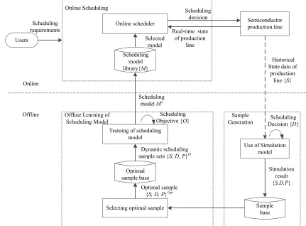
proposed learning-based dynamic scheduling method is shown in Fig. 1. 121
The framework can be divided into three modules. The modules are a) a sample generation 122
module which creates sample production states, and finds the best decision for each performance 123
criterion of interest, b) an offline learning (or training) module that uses the sample data to develop a 124
scheduling library i.e. set of scheduling models, with each scheduling model giving optimal 125
scheduling decisions based on system state for a specified scheduling objective, and c) an online 126
module that uses the scheduling model for decision-making. Since historical data only provide 127
manufacturing system performance for the scheduling decision taken, to develop data that can be 128
used for training purposes, a simulation model is required to predict system performance when 129
alternative decisions are implemented. Here a discrete event simulation model is used, which is 130
based on the actual configuration and behavior of a semiconductor production line. Historical data 131
from an actual line on job sizes, arrival times, machine breakdowns, etc. were described statistically, 132
and used to characterize key simulation inputs. For each simulation trial, all possible decisions were 133
evaluated, and values for the performance criteria of interest were noted. Thus, for every production 134
state, the performance evaluation for every performance criterion is available for every decision. 135
The offline learning module builds a scheduling model for each scheduling objective based on 136
training data, where each dataset includes production states and the corresponding best decision for 137
module can greatly reduce the time consumed for scheduling. The online scheduling module selects 139
a scheduling model from the scheduling model library according to the scheduling requirements of 140
users, and outputs an optimal scheduling decision by inputting real-time state data from the 141
semiconductor production line. 142
A data record in the sample base consists of the production line state (S), scheduling decision 143
(D), and performance (P), given as { , , }. S represents the current state of the production line, 144
working area, machines and jobs obtained from historical data; D is the composite scheduling rule 145
applied, and P is the recorded performance of the given production line found by applying the 146
scheduling decision and running the simulation model for a scheduling period. 147
For the development of the discrete event simulation model for semiconductor production 148
system, please refer to Ye [15]. The discussion here is focusing on the 2nd module i.e. offline learning.
149
Scheduling requirements
Users
Semiconductor production line Online Scheduling
Training of scheduling model
Use of Simulation model Offline Learning of
Scheduling Model
Scheduling modelMo
Historical State data of
production line {S}
Selecting optimal sample Online scheduler
Selected model
Optimal sample {S, D, P}Opt
Dynamic scheduling sample sets {S, D, P}O
Scheduling decision
Real-time state of production
line Scheduling
model library{M}
Optimal sample base
Sample base
Simulation result {S,D,P} Sample
Generation Online
Offline Scheduling
Objective {O} Decision {Scheduling D}
150
Figure 1. The framework of a dynamic scheduling system for a semiconductor production line 151
4. A SVR-Based Dynamic Scheduling Model 152
4.1 Generation of training data from sample base
153
Since running the discrete event simulation model is time consuming (e.g. each simulation run 154
takes more than 30 minutes for a production line with more than 200 steps and 800 machines when 155
processing 80000 wafers), it is infeasible to search for optimal scheduling decision (i.e. weights in a 156
composite rule) using the search algorithm for a production state. To address this, response surface 157
methodology (RSM) is used here. If a model for the response surface exists as a function of the 158
weights/parameters, values may be selected to optimize the composite rule. Such an approach 159
involves three steps: i) running trials of a “process” that depends on several variables (securing 160
“experimental” data), ii) statistical modeling of the experimental data to secure a predicted response 161
surface [16], and iii) using the predicted response surface to select variable settings that optimize a 162
response. Here the weights, ( = 1,2, … , ), are the variables of interest and the response is a 163
multi-objective measure corresponding to scheduling objective. It is desired to find the levels of the 164
(variable settings) for each production state. The performance of the composite rule is evaluated for 166
each trial to obtain a response. A second-order model (shown in Eq. (4)) is then developed for the 167
response as a function of the variables/weights: 168
= + ∑ + ∑ ∑ , (4)
where β ( 0, and ) are estimated parameters. Once the experimental data have been 169
obtained, the form shown in Eq. (4) is fit to the data to obtain the predicted response surface. Then, 170
the combination of weight values, ω∗(i = 1,2, … , k), that optimize production performance may be 171
obtained via calculus from Eq. (4). This set of weight values provides the optimal composite 172
scheduling rule. In this paper, we use design expert software to find the optimal weight for a 173
production state, and then build the optimal ample base. 174
4.2 Development of scheduling models
175
A scheduling decision here is a composite scheduling rule and can be represented by the 176
weights of simple heuristic scheduling rules ( ∈ 0,1 and ∈ ). The scheduling model needs to 177
determine the weights according to the production line state, it is different to those that need to 178
select a scheduling rule from a defined rule set. The scheduling problem then becomes a regression 179
problem as the training datasets cannot cover all the possible production line states. Support vector 180
regression (SVR) is used to build the scheduling model due to its high regression accuracy and its 181
high generalization ability, even when used for problems with a small sample size. Assuming there 182
is a sample set {( , )| ∈ , ∈ , = 1,2, … , }, the nonlinear mapping, ( ), of input, , is 183
built and then the regression function is generated as follows: 184
( ) = ∗∙ ( ) + , (5)
where ∗ and are the weight vector and bias or offset, respectively. The quadratic program 185
is used to solve the problem and minimize the loss function as shown in the Eq. (6) [17]. 186
( ( ) − ) = 0, | ( ) − | ≤
| ( ) − | − , | ( ) − | ≥ , (6)
we can obtain the optimal Lagrange multipliers and ∗ , then acquire the linear regression 187
function in a high-dimensional space, as shown in Eq. (7), where ( , ) is the kernel function. 188
Campbell et al.[18] provide more detail on the SVR method. 189
( ) = ∑ ( − ∗) ( , ) + , (7)
For the scheduling of a semiconductor production line, the input vector = ( , , , , … , , )
190
is a set of production feature values that describe production state; the output vector = 191
( , , , , … , , ) is a set of rule weights of a given scheduling decision in Eq. (3). Based on a sample
192
set {( , )| ∈ , ∈ , = 1,2, … , }, a regression function can be obtained as shown in Eq. (7). 193
So, a composite scheduling rule can be represented by vector ( ) for any given production state, 194
. 195
Given the background provided above for developing a regression model for the scheduling 196
decision, attention now shifts to outlining the stepwise procedure for creating a dynamic scheduling 197
model. There are four steps to build a dynamic scheduling model of a semiconductor production 198
line using SVR. 199
Step 1: Normalizing sample data. For one production feature, , of -th element of -th
200
data record for example, the normalized equation is shown as follows: 201
, = , ,
, , , (8)
where , and , are the maximum and minimum values of , ( = 1, ⋯ , ) in the
202
Step 2: Creating the training sample set and the test sample set. There is a total of optimal 204
samples in the sample set, from which we randomly build training set and test set , 205
respectively accounting for 4/5 and 1/5 of the total sample. 206
Step 3: Training a SVR based scheduling model. Use training set to train a SVR based 207
scheduling model with the radial basis function (RBF) kernel, which is ( , ) = (− ‖ − ‖ ). 208
The penalty factor and the variance of the kernel function are selected to achieve the highest 209
regression accuracy of the model through cross-validation. Based on this, a SVR based scheduling 210
model is created. When the performance of several SVR models is the same or similar, the one with 211
the smallest value is chosen to reduce the complexity of the algorithm. 212
Step 4: Evaluating the model. The created model is evaluated with test set . If the prediction 213
accuracy is in the error range defined based on experience, the model is the one needed, otherwise, 214
return to step 3 and retrain the scheduling model. 215
Once the scheduling model is established, the focus may shift to evaluating the performance of 216
the model, and there are many ways to evaluate the accuracy of the created scheduling model. Here, 217
mean square error (MSE) is used to evaluate the mean error of the scheduling model, which is 218
acquired through Eq. (9): 219
MSE = ∑ ( − ) , (9)
where is the number of the samples in test set , is the predicted weight value and is 220
the real weight value. 221
5 Case Study 222
The proposed method using optimized composite rules is tested on a real semiconductor 223
production line, which produces 5-inch and 6-inch wafers in Shanghai. There are more than 800 224
machines, and the average amount of WIP (work in process) is up to 80,000 pieces in the line. With 225
the help of a self-developed scheduling simulation system (FabSimSys, software copyright number 226
from China: 2011SR066503) and expert design v8.0 software, this paper uses the real line production 227
data to obtain sample data. 228
5.1 Selection of experimental data set
229
5.1.1 Production features set 230
Following the work of the Ma’s work[19], 67 production features were selected for analysis and 231
study. One feature selected was the amount of WIP (number of work in process) and others are 232
distribution of machine number and bottleneck machine number. Utilizing these features, it is 233
possible to describe the state of the both the jobs and the machines for every location in the 234
production line. 235
5.1.2 Design of composite rule 236
Several lot attributes were selected to build the composite rule, and are considered when 237
dispatching lots. Based on industry research, the selected attributes are i) the priority of a lot 238
(Priority), ii) the remaining number of steps in a lot (RemainingStep), and iii) the process time 239
constraint. The process time constraint limits the time between two or more production steps for a 240
lot (Q-Time is a parameter, and if a manufacturing process exceeds it, the lot needs to be reworked or 241
scrapped). These attributes reflect the lot urgency, the degree of completeness, and process 242
constraints. The integrated priority is determined by three attributes. Based on the priorities of the 243
three attributes of lot ( ,, ,, ,) and the weights of the three attributes ( , and ), the
244
integrated priority for lot is calculated (see Eq. (10)). The integrated priority is then used for 245
dispatching the lot. 246
5.1.3 Selection of performance indicators 247
In order to optimize the operation of the semiconductor production line, long-term and 248
short-term performance indicators need to be considered as a whole in the research. Based on the 249
specific application, five performance indicators were selected as the optimization objectives for 250
scheduling: mean cycle time of total lots (MCT), total wafer movement amount (MOV), amount of 251
work in process (WIP), production rate (PR) and overall equipment efficiency (OEE) [20]. Among 252
them, MCT and PR are long-term performance indicators, MOV, WIP and OEE are short-term 253
performance indicators. 254
5.2 Parameter settings of the experiment
255
As has been noted, the inputs of the scheduling model are the production features of the 256
semiconductor production line. In order to improve the output accuracy of the model, it is necessary 257
to reduce the number of inputs by reducing the number of production features; this can be achieved 258
by using the genetic algorithm (GA) [19]. The parameters of the genetic algorithm are set as follows: 259
population size is 100, maximum evolution generation is 100 generations, crossover probability is 0.8, 260
and mutation probability is 0.05. 261
The parameters of the SVR algorithm are set as follows: the maximum and minimum values of the penalty 262
parameter are = 32 and = 0; The maximum and minimum values of the variance parameter 263
in the kernel function are = 32 and = 0.
264
5.3 Experiment results and data analysis
265
Following the application of the genetic algorithm to reduce the number of production features, 266
there are only eight production features left. They are WIP_5 (WIP number in 5-inch), PoBW_DF, 267
PoBW_LT, PoBW_DE, PoBW_WT (proportion of WIP in diffusion area, lithography area, dry 268
etching area, wet cleaning area to WIP), NoBL(number of hot lots in the system), NoBL_DF and 269
NoBL_LT(proportion of hot lots in diffusion area and lithography area). Using the eight attributes, 270
different scheduling methods are applied in the operation of the production line and the production 271
performances are recorded and analyzed. 272
For most semiconductor production applications, the diffusion area and lithography area are 273
usually the focus of scheduling, because a diffusion machine is a batch processing unit in which two 274
or more lots are organized to be processed together, and a lithography machine is a bottleneck unit 275
since it is very expensive. Thus, the dynamic scheduling method proposed in this paper and 276
traditional heuristic rules are applied to these two working areas, with FIFO applied to the other 277
working areas. 278
In the experiment, 100 samples were collected and used (as described before). Of these, 80 279
samples were randomly selected as training samples, and the other 20 samples were used as test 280
samples. The simulation model was initialized based on sample data. Different scheduling rules are 281
used to run the model for a scheduling period and the production performance is recorded at the 282
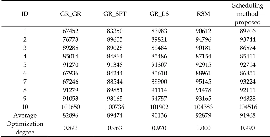
end of each scheduling period. Taking indicator “MOV” as an example, Table 1 provides the 283
scheduling results of 10 samples randomly selected from the test samples using different scheduling 284
rules. 285
In Table 1, columns of 2, 3, and 4 are the results of applying traditional heuristic rules (for 286
example, GR_SPT means the diffusion area uses a GR, or general rule which is an empirical 287
composite rule considering several dispatching factors (e.g. priority, the remaining number of steps 288
and Q-time) in the production line, and the lithography area uses a SPT, or shortest processing time, 289
rule). LS is an abbreviation for least slack, listed as GR_LS in column 3. Column 5 is the result of 290
optimized composite rules whose weights are determined by response surface methodology, and 291
column 6 is the result of applying the proposed scheduling method in this paper. 292
296
Table 1. Performance indicator “MOV” (in step) under different scheduling methods 297
ID GR_GR GR_SPT GR_LS RSM
Scheduling method proposed
1 67452 83350 83983 90612 89706
2 76773 89605 89821 94796 93744
3 89285 89028 89484 90181 86574
4 85014 84864 85486 87154 85411
5 91270 91348 91307 92915 92714
6 67936 84244 83610 88961 86851
7 67246 88544 89900 95145 93224
8 91279 89851 91114 91478 92111
9 91053 93165 94757 93165 94828
10 101650 100736 101902 104383 104516
Average 82896 89474 90136 92879 91968 Optimization
degree 0.893 0.963 0.970 1.000 0.990
298
The better operation of the production line is associated with the larger indicator “MOV” under 299
the same or near same conditions of other production indicators. In the randomly selected 10 300
samples in Table 1, when compared with a single heuristic scheduling rule, the dynamic scheduling 301
method proposed in this paper is more likely to produce an optimal MOV and it can get a better 302
average MOV. Therefore, the dynamic scheduling method proposed in this paper is effective in 303
terms of “MOV” indicator. Because the learning sample is collected according to overall 304
performance of five indicators, some records show that traditional heuristic rules are better than 305
optimized composite rule (its weights determined by RSM) and dynamic scheduling method in 306
terms of the “MOV” indicator. But overall, the proposed dynamic scheduling method is better than 307
traditional heuristic rules. 308
In order to evaluate the overall production performance of the semiconductor production line, 309
the average of each performance indicator for the 20 test samples when using the different 310
scheduling methods was determined. These results are shown in Table 2. 311
Table 2. The average of production performance indicators under different scheduling methods 312
Scheduling
decisions GR_GR GR_SPT GR_LS RSM
Scheduling method proposed
MCT(day) 44.86 44.97 44.76 46.38 45.81
PR(%) 0.3267 0.3338 0.3322 0.3561 0.3523
MOV(step) 85231 89569 90383 92868 92011
WIP(piece) 72051 72046 72048 72030 71186
OEE(%) 0.2917 0.3072 0.3097 0.3202 0.3114 313
Table 2 indicates that MCT, MOV and OEE are most affected by differing scheduling methods. 314
The MCT under the heuristic scheduling rule is better than the one under the proposed dynamic 315
scheduling method while the MOV and OEE are otherwise. The semiconductor production cycle is 316
very long (more than 40 days in the test case) and the scheduling interval time relatively short (only 317
4 hours in the test case in practice), so dynamic scheduling has little effect on MCT. In order to 318
analyze the effect of different scheduling methods on 5 performance indicators, the above 5 319
simplicity, it is assumed that they have equal weight (i.e. weight =0.2 for each indicator), a condition 321
that was also done for the previous sample generation. Once these conditions are applied, a 322
comprehensive value can be obtained that reflects a variety of production performances. Those 323
values are given in Table 2. 324
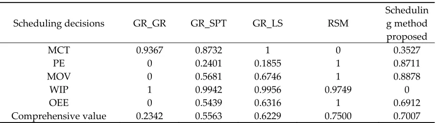
The normalization process is as follows: for a performance indicator, the maximum value is set 325
to “1”, the minimum value is set to “0”, and the other value is set to between “0” and “1” depending 326
on its position between the maximum value and the minimum value. That is, all the performance 327
indicators are normalized. The comprehensive value is weighted sum of normalized value. The 328
greater the comprehensive value, the better the overall performance will be. Table 3 shows that 329
among the four scheduling methods (GR_GR, GR_SPT, GR_LS and the proposed scheduling 330
method), the value for the proposed scheduling method is the largest, and that for the traditional 331
heuristic rule GR_LS is the next largest. Therefore, considering the overall optimization of the five 332
production performance indicators, the dynamic scheduling method proposed in this paper 333
represents a significant improvement over simple heuristic rules in most circumstances, with a slight 334
loss of comparable productivity in some instances. When applying a single heuristic rule, the 335
scheduling rule does not change with the state of the production line. In other words, it does not 336
consider whether the applied scheduling rules match the current state of the production line or not, 337
while the dynamic scheduling method considers it. As a result, the overall performance is worse 338
than that provided by the dynamic scheduling method. 339
Table 3. Normalized value and comprehensive value of the five performance indicators under 340
different scheduling methods 341
Scheduling decisions GR_GR GR_SPT GR_LS RSM
Schedulin g method proposed
MCT 0.9367 0.8732 1 0 0.3527
PE 0 0.2401 0.1855 1 0.8711
MOV 0 0.5681 0.6746 1 0.8878
WIP 1 0.9942 0.9956 0.9749 0
OEE 0 0.5439 0.6316 1 0.6912
Comprehensive value 0.2342 0.5563 0.6229 0.7500 0.7007
342
6 Conclusion 343
Often in industry, a simple dispatching rule cannot meet actual production demand. To 344
improve production, a composite dispatching rule is proposed that considers various factors. This 345
rule can change rule parameters dynamically to meet the requirements of different production states 346
of a production line. One way to realize dynamic scheduling in an actual semiconductor 347
production line is to use a machine learning method. Such a method obtains dynamic scheduling 348
knowledge from optimized scheduling samples, and then utilizes the appropriate dispatching rules, 349
which can be selected to optimize the performance of the production line according to its state. For 350
this purpose, a dynamic scheduling method based on SVR was studied. A real time optimal 351
scheduling strategy was obtained using this method. This method was tested on a 5-inch and 6-inch 352
semiconductor production line. The experimental results show that using a scheduling method 353
based on composite rules gives an obvious improvement in production performance when 354
compared with a single heuristic rule. 355
Acknowledgments: This paper is supported in part by National Nature Foundation of China (No. 51475334, 356
71690234). 357
Author Contributions: Ma, Y.M. and Qiao, F. proposed the idea, implemented experiments and wrote the 358
manuscript; Zhao, F. supervised the study and the manuscript writing process; Sutherland, J. co-supervised 359
Conflicts of Interest: The authors declare no conflict of interest. 361
References 362
1. Mouelhi-Chibani, W. ;Pierreval, H. Training a neural network to select dispatching rules in real time. 363
Computers & Industrial Engineering 2010, 58(2):249–256, DOI: 10.1016/j.cie.2009.03.008. 364
2. Priore, P.; Gomez, A.; Pino, R.; Rosillo, R. Dynamic scheduling of manufacturing systems using machine 365
learning: An updated review. Artificial Intelligence for Engineering Design, Analysis and Manufacturing 366
2014, 8(1):83-97, DOI: 10.1017/S0890060413000516. 367
3. Shiue, Y.R.; Guh, R.S. and Tseng, T.Y. Study on shop floor control system in semiconductor fabrication by 368
self-organizing map-based intelligent multi-controller. Computers & Industrial Engineering 2012, 62(4): 369
DOI: 1119-1129, 10.1016/j.cie.2012.01.004. 370
4. Tsai, C.J.; Huang, H.P. A real-time scheduling and rescheduling system based on RFID for semiconductor 371
foundry FABs. Journal of the Chinese Institute of Industrial Engineers 2007, 24(6): 437-445, 372
DOI: 10.1080/10170660709509058. 373
5. Olafsson, S. ; Li, X.N. Learning effective new single machine dispatching rules from optimal scheduling 374
data. International Journal of Production Economics 2010, 128(1):118-126, DOI: 10.1016/j.ijpe.2010.06.004. 375
6. Ma, Y. M.; Chen, X.; Qiao, F. The Research and Application of a Dynamic Dispatching Strategy Selection 376
Approach based on BPSO-SVM for Semiconductor Production Line. The 11th IEEE International 377
Conference on Networking, Sensing and Control (ICNSC2014), Florida, USA, 7-9 April 2014; 74-79. 378
7. Qiao, F.; Ma, Y. M.; Gu, X. Attribute selection algorithm of data-based scheduling strategy for 379
semiconductor manufacturing. IEEE International Conference on Automation Science and 380
Engineering,(CASE 2013),Madison, WI, USA , 17-20 Aug. 2013; 410-415.. 381
8. Li, L.; Sun, Z.J.; Zhou, M. et al. Adaptive Dispatching Rule for Semiconductor Wafer Fabrication Facility. 382
IEEE Transactions on Automation Science and Engineering 2013, 10(2):354-364, 383
DOI: 10.1109/TASE.2012.2221087. 384
9. Lee, Y.F.; Jiang, Z.B.; Liong, H.C. A smart adaptive production control system for semiconductor foundry 385
fab. The 8th World Multi-conference on System, Cybernetics and Informatics (SCI 2004), Florida, USA, 386
18-21 July 2004. 387
10. Pickardt, C.W. ; Hildebrandt, T; Branke, J ; Heger, J. Evolutionary generation of dispatching rule sets for 388
complex dynamic scheduling problems. International Journal of Production Economics 2013,145(1):67–77, 389
DOI: 10.1016/j.ijpe.2012.10.016. 390
11. Bouri, A.E. ; Amin, G.R. A combined OWA-DEA method for dispatching rule selection. Computers and 391
Industrial Engineering 2015, 88:470-478, DOI: 10.1016/j.cie.2015.08.007. 392
12. Yu,Y.H.; Wang, Y.H. Design and Implementation of a Real-Time Job shop Scheduling System. 393
International Asia Conference on Industrial Engineering and Management Innovation (IEMI2012), Beijing, 394
China, August 10, 2012 - August 11, 2012. 395
13. Chen, T. An effective dispatching rule for bi-objective job scheduling in a wafer fabrication 396
factory—considering the average cycle time and the maximum lateness. The International Journal of 397
Advanced Manufacturing Technology2013, 67 (5): 1281-1295, DOI:10.1007/s00170-012-4565-6. 398
14. Dabbas, R.M; Fowler, J.W. A new scheduling approach using combined dispatching criteria in wafer 399
fabs. IEEE Transactions on Semiconductor Manufacturing 2003;16:501-510, DOI:10.1109/TSM.2003.815201. 400
15. Kai, Y.; Qiao, F.; Ma, Y.M. General structure of the semiconductor production scheduling model. Applied 401
Mechanics and Materials 2010, 20-23: 465-469. 402
16. Devor, R.E.; Chang, T.; Sutherland J.W. Statistical Quality Design and Control: Contemporary Concepts 403
and Methods, 2nd. Prentice Hall: New York, USA, 2006; ISBN:9780130413444. 404
17. Huang, T.M.; Kecman, V.; Kopriva, I. Kernel Based Algorithms for Mining Huge Data Sets. Springer Berlin 405
Heidelberg, 2006. ISBN:3540316817, 9783540316817. 406
18. Campbell C; Ying Y. Learning with support vector machines. Synthesis Lectures on Artificial Intelligence 407
and Machine Learning 2011,10: 1-95, DOI: 10.2200/S00324ED1V01Y201102AIM010. 408
19. Ma, Y.M.; Qiao, F.; Chen, X. A dynamic scheduling approach based on SVM for semiconductor 409
production line. Computer Integrated Manufacturing System 2015, 21(3):733-739,. 410
DOI: 10.13196/j.cims.2015.03.018. 411
20. Jiang, Z.B. Modeling and Optimal Scheduling Control of Semiconductor Manufacturing System. Shanghai 412