Article 1
Flood Mitigation Techniques—A New Perspective
2
for the Case Study of Adayar Watershed
3
Vidyapriya V. 1*, Ramalingam M. 2 4
1 Research Scholar, Institute of Remote Sensing, Department of Civil Engineering, Anna University, Chennai, 5
Tamil Nadu; 6
E-Mails:[email protected]. 7
2Principal, Jerusalem College of Engineering, Velachery Main Road, Chennai, Tamil Nadu; 8
E-Mails:[email protected]. 9
* Author to whom correspondence should be addressed; E-Mail: [email protected]; Tel.: +9952940236. 10
Abstract: Mostly populous city like Chennai is subjected to frequent flooding due to its complex 11
nature of natural and man-made activities. From the analysis of the past records of flood events of 12
1943,1976,1985,2005 and 2008,it has been observed Adayar watershed is subjected to cataclysmic 13
flooding in low-lying areas of the city and its suburbs because of inoperativeness of the local 14
drainage system, rainfall associated with cyclonic activity, topography of the terrain, encroachments 15
along the floodplain, hugh upstream flow discharge into the river and the highly impervious area 16
which blocked the runoff to flow into the storm water drainage. After looking into these problems 17
of flooding, a study have been conducted on Adayar watershed to develop a 2D hydrodynamic 18
model for the two scenarios of existing condition of storm water drainage network and revised 19
conditions of storm water drainage network using high resolution Lidar DEM to assess the volume 20
of runoff with respect to time and duration on flood peaks for the two flood events of 2005 and 21
2015.Secondly to develop a 1D flood model to predict the river stages during peak floods using 22
MIKE 11 for the Adayar watershed. Thirdly to integrate the coupled 1D and 2D model using 23
MIKEFLOOD for assessing the extent of inundation in the floodplain area of Adayar river. Finally 24
results from the integrated model have been validated and the results found satisfactory. As a part 25
of mitigation measures, two flood mitigation measures have been adopted. One measure such as 26
revised storm water drainage system which enhances the flood carrying capacity of the drains and 27
results in less inundated area which solves the problem of urban flooding and second measure such 28
as regrading the river bed which reduces the floodplain inundation around the adjacent area of the 29
river. After adopting these measures, the river is free to flow into the sea without any blockades. 30
Keywords: urban flood; river flood; hydrodynamic model; high resolution dem; flood mitigation 31 measures 32 33 1. Introduction 34
At current; the population of the Chennai city is 46.81% as per the census of India 2011. In the 35
Chennai city, the urban population is expected to increase by 10.129 million in 2025 from 7.557 million 36
in 2010 and 16.278 million in 2050. Cohen [4] predicted by the year 2030 it is expected that 61% of the 37
world’s population of around 5 billion peoples will be living in urban areas. The increase in 38
population results in industrial and urban development. So, by looking on the urban development in 39
mind the flood carrying capacity of the storm water drains has to be designed for the future 40
conditions in order to receive high intensity of rainfall. 41
Urbanization along with heavy rainfall is the cause of flooding in the Chennai city. Since 42
urban area is closely spaced it is advantageous to apply a high resolution DEM data for accurate 43
discrimination of urban features in the flood modelling. Plentiful researches across the world have 44
applied LiDAR data for flood Modelling studies. A study by Jon Derek Loftis et al. [9] conducted at 45
NASA Langley Research Center on sub-grid modelling technology by incorporating high-resolution 46
lidar-derived 5m sub- grid elevation data for the hydrodynamic modelling to resolve detailed 47
topographic features for the generation of runoff .This helps in resolving ditches and overland 48
drainage infrastructure at Langley Research Center often accompanied with tropical storm systems. 49
The results from the model with a NASA tide gauge during Hurricane Irene yielded a good R2
50
correlation of 0.97, and root mean squared error statistic of 0.079 m. The sub-grid model more 51
accurately predicts the horizontal maximum inundation extents within 1.0–8.5 m of flood sites 52
surveyed. Another study by Helen Dorn et al.[7] on comparison of different data sets such as LIDAR 53
data, Orthomap, Open street Map and official landuse data are chosen for surface roughness map 54
generation for accurate prediction of flood. From the comparison of the data, it is found Lidar is best 55
suitable for mapping the roughness map as it avoids the data fusion between the features 56
Various researches have been studied on the impact of urbanization in urban flooding using 1D 57
hydrodynamic models, to simulate flow in sewer pipes for estimation of runoff. Recently, advanced 58
software such as MIKE URBAN storm-water model a physical based GIS integrated model is applied 59
by Chingnawan [3] to solve the pressurized flow using the continuity and momentum equation for 60
Modelling the overland flow for a closed and open conduict. 61
Apirumanekul [2] came with an another interesting case study at Dhaka City to analyze the 62
causes of frequent flooding occurring between two networks namely the street and pipe networks 63
using hydrodynamic model. The model describes the exchange of flows between these two systems 64
of pipes and the streets. The flood inundation maps are prepared using the modelling results in a GIS 65
environment to find the best ways of flood mitigation measures by analyzing the problem faced due 66
to inadequate drainage system prevailing. 67
Similarly some of the literatures are chalked out for solving river flooding problems using 68
hydrodynamic model. A study by Agrawal et al.[1] on Bagmoti river located in Sikkim are analyzed 69
using MIKE11 1D hydraulic model to determine the flood extent and flood depth in the river due to 70
embankment failure and high intensity of rainfall. From the interpretation of the model results 71
suitable flood mitigation measures are suggested. Another study by Vinay Nikam et al. [12] on Mithi 72
river located at Mumbai is flooded due to outburst of the river and heavy rainfall which occurred on 73
26th July, 2005.The main aspects generating the flooding are the encroachments and habitat in flood 74
plains of Mithi River. So in order to predict the inundated area a MIKE 11 model was used to simulate 75
the flooding for various rainfall scenarios. Here various structural and non-structural measures have 76
been adopted to improve the flood carrying capacity of Mithi river by widening or deepening the 77
river bed and by providing flood protection wall at the u/s portion of the river. Likewise this study 78
can also be adopted for other cites as well for deciding suitable flood mitigation measures. 79
Finally, the last stage is the mapping of flood inundation area at risk which requires accurate 80
resolution of DEM data which can be performed using scientific tool such as MIKEFLOOD and 81
remote sensing technique. The 2D hydrodynamic model is widely used for simulation in rivers since 82
one-dimensional models fail to provide complete information about the flow field of extensive flood 83
inundation. The application of 2D flood model developed using Mike by DHI 2014c [10] has gained 84
advantage because it is capable for real-time simulations of flooding events in a relatively less 85
computational time at fine resolution. The governing equation of the model is by mass conversion 86
equation. Thus the present study includes the application of MIKE-FLOOD for the Adayar River 87
flood plain. A large number of studies have been examined using this model which is discussed 88
below. 89
A study for Ajoy River, in West Bengal is analyzed by Prashant Kadam et al.[11] using MIKE-90
FLOOD, which integrates the 1-D MIKE-11 model with the 2-D MIKE-21 model for the flood 91
inundation mapping. The simulation of the model was carried out for two monsoon months of year 92
2000 as the flooding was severe during this period. Next, the MIKE-11 hydrodynamic model was 93
calibrated with the Manning’s, n, roughness coefficient and validated with the gauging station. The 94
results from the model for the validation period gave good agreement with observed values. From 95
the conclusion drawn, suitable flood control measures such as flood forecasting, flood warning can 96
Another study of Tuaran river basin in sabah, Malaysia by Janice Lynn [8] for the year 1999 and 98
2000 flood event is analyzed for the flood risk mapping. The main objective of this research was to 99
generate flood inundation map and to provide suitable flood mitigation measures. So in order to meet 100
the objectives, MIKEFLOOD hydrodynamic model was chosen to predict the flood encroachment 101
map. Here, the topographic data with different resolution of DEM’S are tested for accurate prediction 102
of flood inundation extent. Later on, the calibration of the model was executed during the year 1991 103
and 1992 storm events and then validated using the DID’S flood map through questionnaire survey 104
with local residents. Hence, after validating the model it was found fit for further study. Later on, the 105
three flood mitigation solution is adopted to mitigate flood for the selected high risk areas. The 106
proposed solutions for the river are river deepening, levee constructions and the river straightening. 107
Among the solutions the river deepening was found best for curtailing the effects of flooding in the 108
upstream of the river. 109
2. Study area 110
Chennai City, one of the metropolis in India is the capital of Tamil Nadu. Chennai metropolitan 111
area (CMA) covers an area of 1189 sq.km which lies along the east coast of Southern India. The study 112
area covers Adayar watershed of 42.84 sq.km. It lies between the North Latitudes 13°1’8.513’’ N and 113
13°3’29.645’’N and East Longitudes 80° 11’9.106’’E and 80°15’54.819’’E. Figure (1) depicts the study 114
area map. The Chennai city is bounded by Thiruvallur district in the north and west, Kancheepuram 115
district in the south and Bay of Bengal in the east. The Chennai climate is mostly hot and dry. The 116
mean monthly temperature is in the range of 33.1 – 37.6°C; while in winter temperature fluctuates 117
between 28.1 – 30.6°C. In the year 2003 the Nungambakkam recorded the highest 45°C on 21, May 118
1910.And the second highest 44.5°C was registered on 22,May 2003(SG&SWRDC,TNPWD,2005).The 119
mean annual humidity is usually 58% to 84% and highest percentage of humidity are observed 120
during October to January and moderate in winter. 121
122
Figure 1 The study area of Adayar watershed 123
3. Methodology 125
In this study three Modelling software were employed for flood inundation mapping and 126
mitigation of flood for Adayar watershed. They are MIKE URBAN-1D model, MIKE 11-1D model 127
and MIKE21-2D. These three models are integrated into MIKE FLOOD software for 2D visualization 128
of flood as shown in the Figure (2). 129
130
Figure 2 Framework of the methodology adopted in the study area 131
4. Mike Urban Model 132
4.1. Governing Equations 133
In this study, the Time-area (TA) rainfall-runoff model is used to estimate the runoff hydrograph 134
based on a given excess rainfall hyetograph. In this model, the watershed is divided into a number 135
of sub-watersheds separated by isochrones; i.e. the isolines of equal travel time to the outlet. This 136
procedure is known as time area histogram. The method for the generation of the runoff hydrograph 137
is shown in Equation (1): 138
= ∑ (1)
139
Where j= Time step number, Q= Runoff discharge, E= Excess rainfall intensity, A = Area bounded 140
by the isochrones 141
The imperviousness percentage of the watershed for each sub-catchment according to the 142
percentage of different land use surfaces is calculated using the formula as shown in the Equation 143
(2): 144
Where φ=imperviousness of the whole sub-catchment, φi imperviousness of each type of surface, 146
Ai area of each surface. 147
Later, the initial loss and hydrological reduction factor were assumed to be to 0.6 mm and 0.90 148
respectively in all the sub-catchments from the literature relating to Indian watershed condition is 149
given by Deepak Singh Bisht et al. [5]. And at last the time of concentration (Tc) for each sub catchment 150
is computed using Kirpich’s formula as shown in Equation (3): 151
TC=0.01947*L 0.77 / S-0.385 (3) 152
Where L is the length of the drains and S is the slope of the catchment. The runoff obtained from the 153
catchment is then fed as input to the storm water drainage network for computing flood carrying 154
capacity of the drains. 155
The MOUSE Model is a computational tool for the computation of one-dimensional unsteady 156
flows in sewer networks with alternating free surface and pressurized flow conditions. The 157
computation is based on solving the vertically integrated equations of conservation of continuity and 158
momentum. 159
The general equation of continuity of mass is given by Equation (4) as: 160
+ = 0 (4)
161
And the general equation of momentum is given by Equation (5) as: 162
+ (∝ ) + g *A + g *A If = g *A Io (5) 163
Where: Q = Discharge (m2s-1), A = Flow area (m2), y = flow depth (m), g = acceleration of gravity 164
[ms2], x = Distance in the flow direction (m), t = time, [s], α = velocity distribution coefficient, Io= 165
bottom slope, If= friction slope.
166
The friction loss in the pipe is calculated by Equation (6) as: 167
= (6) 168
Where: τ = tangential stress caused by the wall friction, [Nm-2], ρ = density of water, [kgm-3], R = 169
hydraulic radius, [m]. 170
5. MIKE 11 River Hydrodynamic model 171
5.1. Governing equations for hydraulic model 172
MIKE 11 is a user friendly, fully dynamic, one dimensional hydraulic model used for simulating 173
the water flows in the river. The MIKE 11 is an implicit finite difference model and a fully dynamic 174
one dimensional unsteady flow equation used for the computation of water surface profile and flood 175
discharge at the selected location of the river. Danish hydraulic Institute (DHI) of Water and 176
Environment has developed this one dimensional hydro-dynamic model with other supporting 177
modules like MIKE Zero, GIS, MIKE FLOOD, etc. for surface runoff, channel flow, sediment 178
transport, water quality Modelling in the watershed. High order Dynamic Wave Method is used for 179
unsteady 1D channel routing in this study. Non-linear Saint Venant equations are used here for 180
conservation of mass, volume, momentum and continuity of flow. The equation for conservation of 181
mass is given by Equations (7) and (8) as: 182
. . − . + = . . = . . (7) 183
+ = (8) 184
Equation for Conservation of Momentum equation is given by Equation (9) as: 185
+ . (∝. ) + ℊ. . + . | |. .ℛ= 0 (9) 186
Where: Q = Discharge, A = flow area, Q = lateral inflow, h = stage above datum, C = Chezy resistance 187
coefficient, R = hydraulic or resistance radius 188
The solution of the equations of continuity and momentum is based on an implicit finite 189
difference scheme developed by Abbott and Ionescu in 1967. The transformation of Saint Venant 190
Equations is a set of implicit finite difference equations performed in a computational grid consisting 191
computed at each time step as shown in the Figure 4.8. The computational grid is generated 193
automatically by the model on the basis of the user requirements. Q-points are always placed midway 194
between neighboring h points, while the distance between h-points may differ. 195
5.2. Delineation of Adayar River network 196
In the present study, Adayar river network are imported from the Arc GIS software by using 197
ortho photo imagery as a background. In MIKE 11, the river network acts as a system of points 198
interconnected in between branches. Water levels (h) and discharges (Q) are calculated along the 199
river branches as a function of time.The Adayar river cross section data describes the shape of the 200
stream bed cross section obtained from the field survey by using (x, z) co-ordinates.The discharge is 201
computed using the Manning’s equation is given by Equation (10) such as: 202
Q = M R 2/3 S0 ½ A (10) 203
Where: M = Resistance number, R= Hydraulic radius, S0= bed slope, A= cross sectional wetted area 204
calculated by iteration and it is placed in the cross section table of MIKE 11HD when a certain level 205
accuracy is reached (10−3). 206
6. E 21- 2D Overland flow model 207
MIKE-21 is a Modelling system for 2D free surface flows developed by DHI 2000a [6]. The model 208
is capable of simulating the water level and flows in response to a variety of forcing functions in 209
coastal areas. The hydrodynamic (HD) module is the basic module in the MIKE 21 Flow model. It 210
solves the fully, time-dependent, non-linear equations of continuity and conservation of momentum 211
as represented by Equations (11) and (12), respectively, as given below 212
+ + = (11)
213
+ + + ℎ + − ℎ + ℎ + − +
214
( ) = 0 (12) 215
where = surface elevation (m), t= time (sec), p= flux density in x direction (m3/s/m), x, y = space 216
coordinates (m),d= time-varying water depth (m), h= water depth (m), g= acceleration due to gravity 217
(m/s2), C= Chezy resistance coefficient (m1/2/s), Ωq = Coriolis parameter (s_1), ρw = density of water and 218
f(V) = wind friction factor. 219
The MIKE-21 resolves the solution using an implicit finite difference scheme of second-order 220
accuracy.MIKE-21 model requires input parameters such as bathymetry or terrain elevation which 221
contains the information regarding the elevations of the flood plain. The Digital Elevation Model, 222
obtained from Lidar-DEM are used for the study area. The resolution of the input bathymetry was 223
10m x10 m, so the computational distance was 10 m and the time step adopted was 3 seconds for the 224
simulations. The remaining of the input parameters such as the flood plain roughness coefficient 225
(Manning’s n) as 0.038, flooding depth and drying depth as 0.02 m and 0.03 m are provided in the 226
model. Figure 4.13 shows the representative area of the Lidar-DEM derived bathymetry used in 227
MIKE-21 covering the study area of the Adayar river catchment. 228
7. Integration of MIKE11-1D and MIKE21-2D using MIKE FLOOD software 229
The MIKE-11 river network was connected to the MIKE-21 bathymetry using the lateral link 230
option available in the MIKE-FLOOD. The river bank was dynamically linked with the MIKE-21 grids 231
using a cell-by-cell approach. Whenever the overflow takes place from the 11model, the MIKE-232
21 model calculates the discharge over each cell using weir formula 1. The equation for the weir 233
formula 1 is shown in the Equation (13) as: 234
= ℎ [1 − ℎ ℎ ] . (13)
235
Where w = width, C = weir coefficient (1.838), k exponential coefficient (1.5), ℎ = depth of water 236
above weir level upstream (Hus - Hw) and h2 = depth of water above weir level downstream (H ds – H 237
(k0.385) that approaches 0 as h1 approaches h2.The MIKE-11 model has been calibrated for manning n 239
value and validated against observed data. The simulation period for both MIKE-11 and MIKE-21 240
was kept as the same during the year 2005 and 2015.The model computational time step was assigned 241
as 3 seconds, the Courant Number (CR) is given as less than or equal to 1 so as to achieve stable 242
MIKE-FLOOD simulation run in order to aviod stability problems. 243
8. Results and Discussions 244
8.1. MIKE URBAN Model Results 245
The study area, Adayar watershed was divided into eight micro watersheds for building two 246
scenarios such as existing storm water drainage system and the revised storm water drainage system 247
for assessing the runoff by using MIKEURBAN model as shown in the Figure (3). 248
249
Figure 3 Ilustration of the Adayar watershed in the MIKE URBAN model 250
The results from the model can be viewed in the MIKE View module. The flood inundation maps 251
are prepared by integrating 1D MOUSE model and 2D MIKE 21 model using MIKE FLOOD software. 252
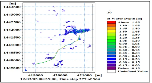
The flood depths and flood extent of the flooded area are generated for the eight micro watersheds. 253
The display of flood inundation maps for one micro-watershed for the year 2005 and 2015 are shown 254
in the following Figures of (4) and (5). 255
The inundated areas of the central Buckingham canal watershed are cathedral road, Masilamani 256
street, sivasamy salai, Muntakaniyamman koil street, Thiruvenkadam street, Luz church road, Sir CV 257
Raman road, Pritiivi avenue. By comparision, the flood inundated area in the year 2015 is more than 258
260
Figure 4 Flood inundation map for the Central Buckingham Canal watershed for the year 2005 261
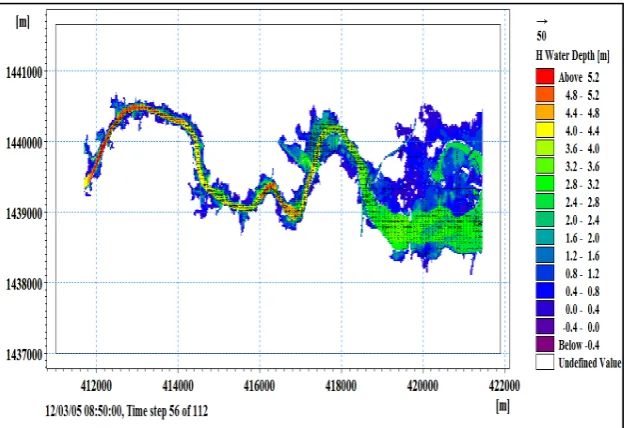
262
Figure 5 Flood inundation map for the Central Buckingham Canal watershed for the year 2015 263
Later on, runoff hydrograph for eight watersheds for two scenarios namely existing drains and 264
revised drainages for the flood event 2005 and 2015 are calculated as shown in the Table 1. From the 265
Table (1), it is clear after revising the size of the storm water drain more than 50% of the flood water 266
have been discharged into the river which alleviates the flooded road. 267
Table 1 Runoff hydrograph of Adayar watershed for the year 2005 and 2015 269
Name of the watershed
Runoff hydrograph for
Existing Drainage 2005 (m3/s)
Runoff hydrograph for Existing Drainage 2015 (m3/s)
Runoff hydrograph for Revised
Drainage 2005 (m3/s)-
Runoff hydrograph for
Revised Drainage 2015 (m3/s)
K.K Nagar 85.41 134.34 110.06 211.17
Jafferkhanpet 69.55 118.20 88.97 141.06
Mambalam 193.86 275.23 403.62 685.23
Central Buckhingham
Canal
169.29 227.56 250.68 452.21
Alandur 76.99 127.97 89.71 215.39
Chellamal 33.46 110.51 54.75 174.67
Kotturpuram 54.94 93.87 75.35 113.28
Thiru-vi-ka 64.12 91.58 83.6 148.01
Total 747.62 1179.26 1156.74 2141.02
8.2. MIKE 11 River Flood Model Results 270
The High order Dynamic Wave Method is used for unsteady 1D channel routing in this study. 271
The Non-linear Saint Venant equations are used for conservation of mass, volume, momentum and 272
continuity of flow. The model gives discharge at different cross section, velocity and as well as water 273
level profile at different locations of cross section. The water level surface profiles of Adayar river 274
for the flood event 2005 has attained the highest water level at 3-12-2005 on 09:30:00 AM as shown in 275
the Figure (6). From the Figure (6), it is clear their is overtopping of river banks which inundates 276
adjacent areas. 277
278
Figure 6 Water level profile of Adayar river for surveyed cross-section for the year 2005 (MIKE 11 279
model output) 280
Similarly the water level surface profiles of Adayar watershed for the flood event 2015 has 281
attained the highest water level at 2-12-2015 on 09:30:00 AM as shown in the figure (7). From the 282
Figures of (7), it is clear their is overtopping of river banks across various bridges which inundates 283
285
Figure 7. Water level profile of Adayar river for surveyed cross-section for the year 2015 (MIKE 11
286
model output) 287
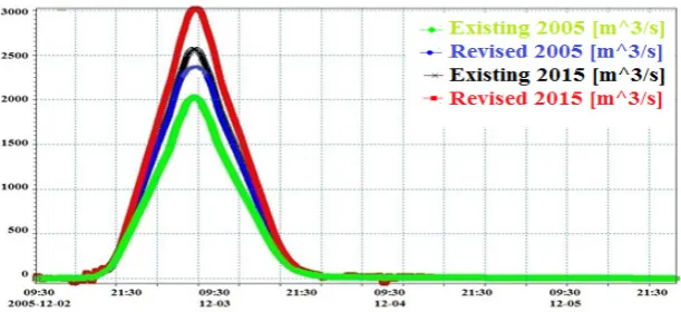
From the model output the flood discharge, flood inundated area and flood depth with respect 288
to duration are found. The flood discharge peak during 2005 for the existing and revised drain on 2nd 289
December 2005 to 4th December 2005 is at 9:30 AM and during 2015 for the existing and revised drain 290
on 1nd December 2015 to 4th December 2015 is at 9:46 AM for the Adayar river at the outlet are 291
presented in the Figure (8). 292
293
Figure 8 Flood Hydrograph for the Adayar river for the year 2005 and 2015 flood event of MIKE 11 294
model 295
From the Figure 8, it is clear that up on revised drainage network more discharge have been 296
mitigated to the river which reduces the urban area being inundated for the year 2005 and 2015. 297
Thus solves the problem of urban flooding. 298
8.3. Model validation using Error Index Statistics 299
The performance of the MIKE 11 model is tested against the observed water level using R2 300
statistics at various locations of the Adayar river during the year 2005 and 2015. The model 301
performance has been validated using the observed and simulated value using statistical method. 302
RMSE is one of the commonly used error index statistics. The RMSE value less than 1 indicates better 303
performance model. The Equation (14) for computing the RMSE is shown as: 304
RMSE = ∑ ( ) (14) 305
Where, yi obs is the observed discharge, yi sim is the simulated discharge and nis the total number of
306
events. 307
The RMSE value of less than one from the model indicates good performance. Since there is lack 308
Hence the model has been validated with the available data. It has been concluded that the simulated 310
water levels by MIKE11 have R2 coefficient of determination as 0.92 for 2005 flood event and 0.89 as 311
for 2015 flood event as shown in the Figure (9) and (10). 312
313
Figure 9 Comparison of Observed and Simulate Figure 10 Comparison of Observed and 314
simulated water level for 2005 flood event water level for 2015 flood event 315
8.4. Flood Mitigation Measure 316
In this present study, the flood mitigation measures have been carried out by two ways such as: 317
Urban flood mitigation, River flood mitigation and flood mitigation into the sea. 318
8.4.1 Urban flood mitigation measure through revised storm water drainage network 319
Floods have been mitigated through revised storm water for eight watersheds. But the results 320
are displayed for one Central buckhingam canal watershed alone. The watershed covers an area of 321
about 6.61 Sq.km. From the results of the model, the total flood volume inundated in the Central 322
buckhingam canal watershed during 2005 flood event was found to be 0.373 MCM. But after the 323
revised size of the drains the flood volume has been reduced to 0.219 MCM. The flood inundated 324
map for the revised drains for the year 2005 is shown in the Figure (11). Likewise the total flood 325
volume inundated in the Central buckhingam canal watershed during 2015 flood event was found to 326
be 0.631 MCM. But after the revised size of the drains the flood volume has reduced to 0.219 MCM. 327
The flood inundated map for revised drains for 2015 flood is shown in the Figure (12). 328
329
Figure 11 Flood Inundation map of revised storm Water drainage network of Central Buckhingham 330
332
Figure 12 Flood Inundation map of revised storm water drainage network of Central Buckhingham 333
canal watershed for the year 2015 334
Some portion of a flood has been mitigated through revised storm water drains. The balance 335
flood volume of 0.154 MCM for 2005 flood and 0.34 MCM for the 2015 year flooded out from the 336
drains has been discharged through surface canal draining into the river. By implementing the 337
suggested mitigation measure, the urban flooding volume has been reduced to great extent. 338
8.4.2. River flood mitigation measure through regarding the channel 339
Now In order to avoid flooding in the river the cross section of the river has been regraded 340
(lowered) to 0.8 m and 1.0 m for the flood event 2005. But the results are displayed for 1.0m regarded 341
channel as shown in the Figures (13). From the results, after regrading the river bed the flood depth 342
has been reduced drastically and the overtopping of the banks have been controlled through this 343
method. 344
345
Figure 13 Water level profile of Adayar river after regrading the cross section by 1.0 m for the year 346
2005 (MIKE 11 model output) 347
Similarly for the flood event 2015, In order to avoid flooding in the river the cross section of the 348
river has been regraded to 0.8 m and 1.0m. But the results are shown in the Figures (14) for 1.0m 349
regarded river bed. From the results, after regrading the river bed the flood depth has been reduced 350
352
Figure 14 Water level profile of Adayar river after regarding the cross section by 1.00 m for the year 353
2015 ( MIKE 11 model output) 354
8.4.3. Flood plain mapping after mitigation of the Adayar River 355
The Adayar river have been completely mitigated after modifying the cross sections at important 356
locations of the bridges. Now, the river has the flood carrying capacity of 1463.48 m3/s discharge for 357
the rainfall of 60 mm peak during 2rd December to 3rd December 2005 without being flooded and 358
2332.64 m3/s discharge for the rainfall of 68 mm peak during 1st December to 3rd December 2015.The 359
following Figures from (15) to (18) shows the inundation map for existing cross section and regraded 360
cross section of Adayar river. 361
362
364
Figure 16 Flood plain mapping of Adayar river for the modified cross section of 1.00 m for the year 365
2005 366
367
Figure 17 Flood plain mapping of Adayar river for surveyed cross section of 1.00 m for the year 2015 368
369
Figure 18 Flood plain mapping of Adayar river for the modified cross-section for the year 2015 370
Similarly, from the above Figures 15-18, it is clear the regarding of the river bed serves as a best 371
9. Conclusion and Recommendations 373
Based on the objective, the Time-area (TA) rainfall-runoff model is used to estimate the runoff 374
volume and to estimate flood depth. The volume of flood for eight Adayar micro-watersheds have 375
been estimated for two scenarios namely existing storm water drainage network and revised storm 376
water drainage network. This study found the runoff volume generated is more in existing drainage 377
network than that of the revised drain as because of the increase in size of the storm water drainage. 378
In order to minimize the urban flood the revised storm drainage is adopted and the conclusions 379
are drawn as follows: 380
Flood has been mitigated in the Adayar watershed through revised storm water drains. From 381
the results of MIKEFLOOD software, the flood discharge into the Adayar river during 2005 flood 382
event was found lesser compared to the 2015 flood event. Ultimately, this flood discharge inundates 383
the Adayar watershed beyond the flood carrying capacity of storm water drainage network. The total 384
runoff volume inundated in the Adayar watershed for the existing drain for the year 2005 is found to 385
be 0.017 MCM and after revised drain the flood volume have reduced to 0.011 MCM. Similarly for 386
the year 2015 the flood volume for the existing drain is found to be 0.022 MCM and after revising the 387
drain the flood volume have reduced to 0.020 MCM. From the results, it clearly shows it is the best 388
mitigation measure for alleviating the flood. The balance flood volume of 0.0053 MCM and 0.0018 389
MCM for the year 2005 and 2015 have been mitigated through surface canal draining into the river 390
and ultimately into the sea. The flat topography of Chennai makes it difficult to carry excess flood 391
water which needs immediate attention for mitigating flood waters. 392
In this study, hydraulic model MIKE 11 were analyzed for floodplain mapping of Adayar river 393
for two flood events of 2005 and 2015. The model is used and is validated against the observed flood 394
depth of 2005 and 2015 flood event. From the model results, the model gave more coefficient of 395
determination having R2 equal to 0.92 for 2005 flood event and R2 equal to 0.89 for 2015 event. The 396
balance flood discharge of 755 m3/s of existing drain and 1,092.11 m3/s of revised drain for 2005 flood 397
event and the balance flood discharge of 889.36 m3/s of existing drain and 701.51 m3/s of revised drain 398
for 2015 flood event from the river and urban sub watersheds has to be discharged in to the sea as a 399
part of flood mitigation measure. 400
After regrading the bed of the river by 1m, the area inundated has been reduced from 14.05 Km2 401
to 6.81 Km2.Hence the suggested mitigation measure is to open the sea mouth during low tide level, 402
removal of sand bar at the sea mouth and control of sediments solves the flood problem. By 403
implementing the suggested measure, the river flood area will be discharged completely into the sea 404
without any blockades for safer livelihood. 405
The study can be improved by incorporating the suggested recommendations. In the heavily 406
developed Adayar watershed, the runoff water must be recognized as a valuable resource and 407
preserve it for the stable ground water table during summer season. For the effective prediction of 408
runoff water the model has to consider population density as well as impervious value from the 409
landuse/ land cover map. Different methods for calculating time of concentration for urban 410
watershed can be attempted and chosen for best urban runoff model. The climate change parameter 411
can be included in the study for the prediction of future flood and Automatic weather rain gauge 412
data can be considered in future at an interval of 1 hour duration rainfall for flood forecasting study. 413
To remove formation of sand bars in the river mouths causing stagnation in Adayar river. Bank 414
protection for the stretch 0.0 to 0.5 km -0.75 meters thick rubble gabion packing on slopes on both 415
sides. Maintenance dredging to maintain the tidal prism. To open the sea mouth during low tide 416
level, removal of sand bar at the sea mouth and control of sediments solves the flood problem. The 417
available surface water can be utilized for augmenting the ground water which can considered for 418
future study. The different methods of ground water conservation are by way of constructing 419
percolation pits, recharge trench, roof water harvesting structures according to the site condition.The 420
Chennai Corporation has initiated to construct rainwater harvesting structure across the Chennai city 421
Acknowledgments: The authors would like to express profound gratitude to Dr. M. Ramalingam, Former 423
Director, Institute of Remote Sensing, Anna University for his guidance, constant encouragement and invaluable 424
support during the research work and DHI (India) Water & Environment pvt ltd. for their guidance on the 425
analysis of hydrodynamic model. 426
Author Contributions: Each author had contributed to this research work. The first author, vidyapriya, had the
427
responsibility of developing and testing the model. The second author Ramalingam helped to analyze the data 428
and made necessary suggestion on this work. 429
Conflicts of Interest: The authors declare no conflict of interest. 430
References 431
1. Agrawal, SK ,; Kharya, AK,;Khattar,R,. Flood Management in Bagmati Basin, Central Water Commission, 432
2001, Bihar, India. 433
2. Apirumanekul,C,. Modelling of urban flooding in Dhaka City, Master Thesis No. WM-00-13, 2001, Asian 434
Institute of Technology, Bangkok. 435
3. Chingnawan, S,. Real-Time Modelling of urban flooding in the Sukhumvit area, Bangkok, Thailand, Master 436
Thesis, 2003, Asian Institute of Technology, Bangkok. 437
4. Cohen B,.Urbanization in developing countries: Current trends, future projections, and key challenges for 438
sustainability, Technology in Society, 2006,28,63-80. 439
5. Deepak Singh Bisht,; Chandranath Chatterjee,; Shivani Kalakoti,; Pawan Upadhyay,; Manaswinee Sahoo,; 440
Ambarnil Panda Miller, N. Modelling urban floods and drainage using SWMM and MIKE URBAN : a case 441
study, Natural Hazards,2016,vol. 84, pp. 749-776. 442
6. DHI,.MIKE-21 Short introduction and tutorial, 2000a, Danish Hydraulic Institute. 443
7. Helen Dorn,;MichaelVetter,;Bernhard Hofle,.GIS-Based Roughness Derivation for Flood Simulations: A 444
Comparision of Orthophotos, LiDAR and Crowd sourced Geo data, Remote sensing,2014,6,1739-1759. 445
8. Janice Lynn Ayog ,. Flood Risk Mapping for flood mitigation and floodplain management in Tuaran River 446
Basin, M.S Thesis, 2005,Perpustakaan Universiti Malaya. 447
9. Jon Derek Loftis ,; Harry V. Wang,; Russell J. De Young ,;William B. Ball. Using Lidar Elevation Data to 448
Develop a Topo bathymetric Digital Elevation Model for Sub-Grid Inundation Modeling at Langley 449
Research Center, Journal of coastal Research, 2016, 76, 134–148. 450
10. MIKE by DHI ,. MIKE FLOOD User Manual, 2014c, DHI Water and Environment. 451
11. Prashant Kadam ,; Dhrubajyoti Sen,. Flood inundation simulation in Ajoy river using MIKEFLOOD.ISH 452
Journal of Hydraulic Engineering, 2012, 18, 129-141. 453
12. Vinay Nikam,;Kapil Gupta,. Flood Resilience study for mithi river catchment in Mumbai, International 454
Conference on flood resilience experiences in Asia and Europe, 2013,Indian Institute of Technology, 455