Pyplis
- A Python Software Toolbox for the Analysis
of SO
2
Camera Data
Jonas Gliß1,2,3*, Kerstin Stebel1, Arve Kylling1, Anna Solvejg Dinger1,4, Holger Sihler5and Aasmund Sudbø3
1 NILU - Norwegian Institute for Air Research, Kjeller, Norway
2 Department of Physics, University of Oslo (UiO), Oslo, Norway
3 Department of Technology Systems, University of Oslo (UiO), Kjeller, Norway
4 Institute of Environmental Physics (IUP), University of Heidelberg, Germany
5 Max Planck Institute for Chemistry (MPIC), Mainz, Germany
* Correspondence: [email protected]; Tel.: +47-94885617
Version October 13, 2017 submitted to Entropy
Abstract:UV SO2cameras have become a common tool to measure and monitor SO2-emission-rates,
mostly from volcanoes but also from anthropogenic sources (e.g. power plants or ships). In the past years, the analysis of UV SO2camera data has seen many improvements. As a result, for many
of the required analysis steps, several alternatives exist today. This inspired the development of
Pyplis, an open-source software toolbox written in Python 2.7, which aims to unify the most prevalent 5
methods from literature within a single, cross-platform analysis framework.Pypliscomprises a vast collection of algorithms relevant for the analysis of UV SO2 camera data. These include several
routines to retrieve plume background radiances as well as routines for cell and DOAS based camera calibration. The latter includes two independent methods to identify the DOAS field-of-view within the camera images. Plume velocities can be retrieved using an optical flow algorithm as well as 10
signal cross-correlation. Furthermore,Pyplisincludes a routine to perform a first order correction of the signal dilution effect. All required geometrical calculations are performed within a 3D model environment allowing for distance retrievals to plume and local terrain features on a pixel basis. SO2-emission-rates can be retrieved simultaneously for an arbitrary number of plume intersections. Pyplishas been extensively and successfully tested using data from several field campaigns. Here, 15
the main features are introduced using a dataset obtained at Mt. Etna, Italy on 16 September 2015.
Keywords:volcanic gases; SO2; remote sensing; UV cameras; image processing; analysis software;
Python 2.7
1. Introduction
Sulfur dioxide (SO2) is a toxic gas emitted by anthropogenic and natural sources (e.g. power 20
plants, ships, volcanoes). The pollutant has impacts on the atmosphere both on local and global scales (e.g. particle formation, radiation budget, e.g. [1], [2]). Furthermore, the monitoring of SO2emissions
from active volcanoes can provide insight into the magma degassing behaviour and hence plays an important role for the development of new risk assessment approaches (e.g. [3], [4], [5], [6], and references therein).
25
The gas composition of the emission plumes can, inter alia, be studied using ground-based passive remote sensing techniques. The column-densities (CDs) of the gases in the plumes are quantified based on the absorption signature carried by scattered sunlight that has penetrated the plume. SO2-CDs,
for instance, can be retrieved at ultraviolet (UV) wavelengths (i.e. around 310 nm) where it exhibits distinct absorption bands. Prominent examples for passive remote sensing instrumentation are the 30
correlation spectrometer (COSPEC, [7]), or instruments based on the DOAS technique (differential optical absorption spectroscopy, [8], e.g. [9], [10]). During the past years, the comparatively young technique of UV SO2cameras has gained in importance, since it enables to study volcanic SO2emissions
at unprecedented spatial and temporal resolution (e.g. [11], [12], [13], [14]). This is particularly helpful to study multiple sources independently (e.g. [15]) or to investigate volcanic degassing characteristics 35
by studying periodicities in the SO2-emission-rates (e.g. [16]). The technique of UV SO2cameras has
seen remarkable improvements in the past years (e.g. [17], [18], [19], [20], [21]) and can nowadays be considered one of the standard methods for ground-based remote sensing of SO2plumes. A drawback,
however, is the low spectral resolution, restricting the technique to a single species and furthermore, requiring external calibration.
40
The retrieval of SO2-emission-rates from the plume imagery comprises several analysis steps
which are summarised in Table1and are illustrated in the flowchart shown in the Appendix FigureA1. Thanks to ongoing developments, today, researchers can choose between several methods for nearly all of the required steps (e.g. cell vs. DOAS calibration, velocity retrieval using optical flow vs. cross-correlation method).
45
Available software solutions include Vulcamera ([22]), the IDL source code provided by [19] and Plumetrack ([23]). The first two programs include routines for cell calibration and cross-correlation based plume speed retrievals. The IDL program also includes a routine to perform a first order correction for the signal dilution effect. The software Plumetrack provides an interface to calculate gas velocities using an optical flow algorithm and can be applied to pre-calibrated SO2-CD images in 50
order to retrieve SO2-emission-rates.
Table 1.Analysis blocks for emission-rate retrievals
Analysis block Quantities Analysis options Sect.
Geometrical calculations ∆s(m) 3.1
Plume background analysis τon,τoff,τAA 3.3
Camera calibration SSO2(m) Cell, DOAS 3.4
Plume speed retrieval hv(m)¯ ·n(m)ˆ i Optical flow, cross-correlation 3.5 Emission-rate ΦSO2 Signal dilution correction 3.6,3.7
Pyplis(Pythonplumeimagingsoftware) is a cross-platform, open-source software toolbox for the analysis of UV SO2camera data. The code is written in Python 2.7 and emerged from the idea
of a common software platform incorporating the most relevant analysis methods, including recent developments. The most important features ofPyplis0.13.4 are (details follow in Sect.3):
55
1. 3D distance retrievals to plume and local terrain features at pixel-level, 2. several methods to retrieve plume background radiances,
3. cell and DOAS based camera calibration including two independent DOAS FOV search routines, 4. cross-correlation and optical flow based plume velocity retrievals,
5. histogram based correction for ill-posed optical flow vectors in low-contrast image regions, 60
6. image based correction for the signal dilution effect,
7. automated emission-rate retrievals along linear plume intersections.
Pypliscomes with numerous example scripts providing an easy and comprehensive introduction into the software. The following Sect.2introduces the technique of UV SO2cameras and the required
analysis steps for SO2-emission-rate retrievals. The implementation of the individual analysis methods 65
is discussed in Sect.3.
2. Methodology
2.1. UV SO2cameras
UV SO2cameras analyse scattered sun light which has penetrated a plume containing SO2gas.
Plume optical densities (ODs)τare retrieved in two wavelength windows of approximately 10 nm
width, using optical bandpass filters. One filter is centred around 310 – 315 nm, where SO2has strong
SO2absorption is weak (SO2off-band). The latter is used to correct for additional broadband light
extinction, for instance, resulting from aerosols or water droplets in the plume. From the retrieved ODs in both channels, the apparent absorbance (AA) of SO2(τAA, e.g. [17]) can be retrieved as
τAA=τon − τoff=ln
I0 I
on
−ln
I0 I
off
, (1)
whereIandI0denote the plume and plume background radiances, respectively, in both channels (on, off). Note that the method requires all additional optical densities in the on and off-band regime to be 70
of broadband nature.
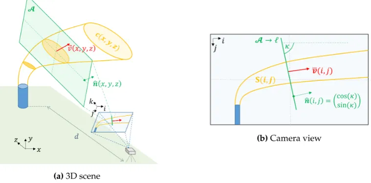
(a)3D scene
(b)Camera view
Figure 1.Measurement geometry - sketched (a) in three dimensions and (b) as the camera sees it. The emission plume is indicated in yellow colours, gas velocities in red. The orientation of the plume cross-section (PCS)A(green colours) is aligned with the camera optical axisk.
2.2. Image analysis - Retrieval of SSO2images
AA images are determined from a set of pre-processed (e.g. dark / offset corrected) plume and background images using Eq.1. Next, the AA images are converted into SO2column-density (CD)
images, where
SSO2(i,j) = Z
Cijc(x,y,z)ds (2)
denotes the SO2-CD in the viewing directionCijof the image pixeli,j.c(x,y,z)is the concentration distribution of SO2in real world coordinatesx,y,z(cf. Figure1a) andds=
p
dx2+dy2+dz2is the
integration differential. 75
The camera calibration (i.e. the conversion of AA values into SO2-CDs) can be performed either
using gas cells (e.g. [11]) or a co-located DOAS spectrometer (e.g. [18]). The latter is more accurate in case aerosols are present in the plume ([18], [24]). The position and shape of the DOAS FOV within the camera images is required in order to perform the DOAS calibration. The FOV can either be measured 80
experimentally (e.g. in the lab) or can be retrieved directly from the field data ([18], [25]). The filter transmission curves shift towards lower wavelengths for non-perpendicular illumination. This leads to an increased SO2sensitivity towards the image edges. A correction for this effect can be performed
2.3. Emission-rate retrieval 85
SO2-emission-ratesΦare retrieved from SO2-CD images by performing a discrete path integration
along a suitable plume cross section (PCS) projected into the image plane, for instance a straight line`
(illustrated in Figure1b). Then,
Φ(`) = f−1 M
∑
m=1SSO2(m)· hv¯(m)·nˆ(m)i ·dpl(m)·∆s(m) (3)
corresponds to the SO2-emission-rate through`, wheremdenotes one of a total ofMsample positions
along`in the image plane and∆sis the integration step length, measured in physical distances on the detector. f is the focal length of the camera,dplis the distance between camera and plume andnˆis the
normal of`.v¯is a 2-vector containing projected plume velocities averaged in the viewing direction. The plume distances dpl can be estimated from the measurement geometry and require 90
information about the camera position and viewing direction as well as the source position and the meteorological wind direction. The gas velocities are usually retrieved from the images directly either using cross-correlation based methods (e.g. [26]) or optical flow algorithms (e.g. [20]).
Eq. 3is equivalent to commonly used retrieval methods (e.g. [11], [24]) and is based on the assumption that over or underestimations of the measured quantities SSO2 and v¯ (e.g. due 95
to non-perpendicular plume transects) cancel out in the emission-rate retrieval. This is a valid approximation for typical measurement conditions (i.e. plume nearly perpendicular to the optical axis, and plume extend small compared to plume distance). However, care has to be taken for unfavourable geometries (e.g. tilted or overhead plume; retrieval close to the image edges) which may require additional corrections (e.g. [27]).
100
If a locally uniform gas velocity can be assumed (i.e. v¯(i,j)→v) and further, a planar PCS is¯
used for the retrieval (i.e.nˆ(i,j)→n) then, Eq.ˆ 3can be further approximated asΦ(`)≈ hv¯·nˆi ·χ(`),
where
χ(`) = f−1
M
∑
m=1SSO2(m)·dpl(m)·∆s(m) (4)
denotes the integrated column amount (ICA) along(`).
2.4. Radiative transfer corrections
Radiative transfer effects may introduce systematic errors in the retrieved emission-rates (see e.g. [28], [29]). The signal dilution effect describes a decrease in the measured CDs due to scattering 105
between instrument and plume. The magnitude of this effect primarily depends on the local visibility (i.e. amount of molecules and particles in the ambient atmosphere) and on the distance between camera and plume. A first order correction can be performed using the atmospheric scattering extinction coefficients in the viewing direction between camera and source (e.g. [12], [30]). The latter can be retrieved, for instance, by studying brightness variations of topographic terrain features in the images 110
as a function of their distance to the instrument ([19]). More complicated radiative transfer issues (e.g. optically thick plumes) require corrections using radiative transfer models (e.g. [24]).Pypliscan correct for the signal dilution effect based on the method suggested by [19].
3. Implementation
In the following, the main features and modules ofPyplisare presented. The API is designed 115
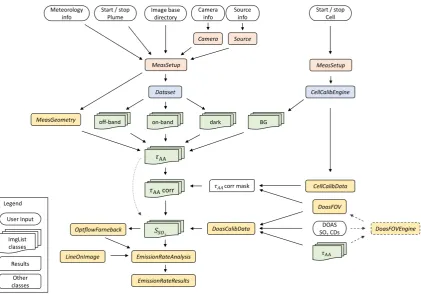
modular using object oriented architecture. It can therefore be used in parts or as a whole. Figure2
illustrates thePyplisAPI for SO2-emission-rate retrievals (see also AppendixD).Pyplisincludes 19
between 06:40 – 07:30 UTC. These data is freely available and can be downloaded from the website (for 120
details see AppendixE.1).
Figure 2. PyplisAPI - Flowchart illustrating the main analysis steps and the corresponding classes of thePyplisAPI for SO2-emission-rate retrievals. Italicdenotations correspond to class names in
Pyplis. Optional analysis steps are indicated by dashed boxes. Setupclasses (red) include relevant meta information and can be used to createDatasetobjects (blue). The latter perform file separation
by image type and createImgListobjects (green) for each type (e.g. on, off, dark). Further analysis classes are indicated in yellow. Note that the routine for signal dilution correction is not shown here (cf. FigureA1).
3.1. Geometrical calculations
Geometrical calculations are performed within an instance of theMeasGeometryclass (part of the
geometry.pymodule). The plume distancesdpl(cf. Eq. 3) can be retrieved per pixel-columniusing intersections of the respective viewing azimuth with the plume azimuth (see Figure3). This requires 125
specification of the camera position, viewing direction and optics (e.g. detector specifications, focal length), source coordinates and meteorological wind direction. The distances are determined based on the horizontal plume distance and the altitude difference between source and camera (i.e. assuming a horizontally aligned plume). It is pointed out, that this approach may be inapplicable for complicated measurement geometries (e.g. overhead plumes), which would require a more detailed knowledge of 130
the plume shape and altitude.
Further features of theMeasGeometryclass include a routine to retrieve the camera viewing direction based on the position of distinct objects in the images (e.g. summit of volcano, cf. Figure3), or the calculation of distances to topographic features in the images (shown in Figure10, for details see 135
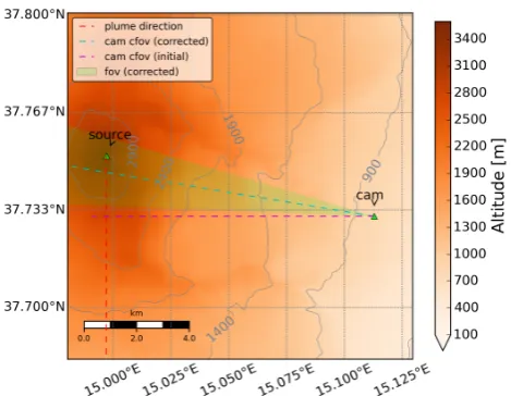
Figure 3. Measurement geometry - 2D overview map of the measurement setup at Mt. Etna from thePyplisexample data. The map includes plume orientation (red dashed line), camera azimuth retrieved using a compass (purple dashed line) and the corrected camera azimuth (blue dashed line) and corresponding FOV (semi-transparent green), retrieved automatically using the positioni, jof the Etna south-east crater within the images and the corresponding coordinates of the crater (longitude, latitude, altitude). The map was generated using aMeasGeometryobject (see Sect.3.1).
be created automatically (as shown in Figure3, see also Figure10c). TheMeasGeometryclass uses the Python Geonum library ([31]) which is briefly introduced in AppendixA.
3.2. Image representation and pre-processing routines
Images are represented by theImgclass (image.pymodule). TheImgclass includes reading routines
140
for all image formats supported by the Python Imaging Library (PIL, e.g. png, tiff, jpeg, bmp) as well as the FITS format (Flexible Image Transport System). It further allows to store relevant meta information (e.g. exposure and acquisition time, focal length, f-number) and includes several basic processing methods (e.g. smoothing, cropping or resizing using a Gaussian pyramid approach). The image data itself is loaded and stored as a 2D-NumPy array within anImgobject. Automatic dark and
145
offset correction can be performed as described in AppendixB.Imgobjects can be saved as FITS files at any stage of the analysis (e.g. dark corrected image,τAAimage, calibrated SO2-CD image).
3.3. Retrieval of plume background radiances
The calculation of the OD images in both wavelength channels requires the retrieval of the sky-background intensitiesI0behind the plume (cf. Eq.1). Theplumebackground.pymodule provides 150
several alternatives to retrieve the background intensities, either from the plume images directly or using an additional sky reference image (I0-image). For the latter, several methods are available to correct for offsets and non-uniformities in the sky-background between the plume andI0-image. The corrections are based on suitable sky-reference-areas in the plume image (rectangles or profile-lines, cf. Table2) and use 1stor 2ndorder polynomials to model theI0-image such, that the corresponding OD 155
image satisfiesτ=0 within the specified sky reference areas.
If noI0-image is available, the plume background radiances can also be estimated from the plume images directly using a masked 2D polynomial surface fit. The required mask specifies clear-sky image pixels which are considered during the fit. The mask can either be provided by the user or can be retrieved automatically using the methodfind_sky_background.
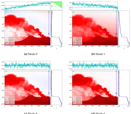
(a)Mode 0 (b)Mode 1
(c)Mode 4 (d)Mode 6
Figure 4.Plume background modelling - Four example on-band OD images (τon) determined using background modelling modes 0 (polynomial surface fit) and 1, 4 and 6 (based onI0-image, cf. Table2). Horizontal and vertical profiles are plotted on the top and on the right, respectively. The top-left plot (Mode 0) further includes the mask specifying sky-reference pixels (green area) which was used for the polynomial surface fit. The plume and background images used for the displayed examples were recorded at 07:06 UTC and at 07:02 UTC, respectively.
ThePlumeBackgroundModelclass (part of plumebackground.py) provides high level access to eight default methods for the background retrieval. The methods are summarised in Table2. Figure4shows four example plume on-band OD images calculated using the modelling modes 0, 1, 4 and 6. It is not intended to give a recommendation for a “best” method here, as this strongly depends on the data 165
Table 2.Available plume background modelling modes of thePlumeBackgroundModelclass (cf. names of sky reference areas in Figure4)
Corrections
Mode I0-img Scaling Vertical Horizontal
1 yes scale_rect
2 yes scale_rect ygrad_rect (linear) 3 yes scale_rect vert. profile (quadratic)
4 yes scale_rect ygrad_rect (linear) xgrad_rect (linear) 5 yes scale_rect vert. profile(quadratic) xgrad_rect (linear) 6 yes scale_rect vert. profile (quadratic) hor. profile (quadratic) 0 no Masked 2D polynomial surface fit
99 yes None (useI0-img as is)
3.4. Camera calibration
The camera calibration can either be performed using data based on cuvettes filled with a known amount of SO2-gas, or using plume SO2-CDs retrieved from a co-located DOAS spectrometer (cf. 170
Table1).
3.4.1. Calibration using SO2cells
(a)Cell search result on-band (b)Example calibration curves
Figure 5.Cell calibration - (a) shows the output of the automatic cell search routine (included in the
CellCalibEngineclass). (b) shows example calibration curves forτon,τoffandτAAimages for the image center pixel from the dataset shown in (a).
Cell calibration can be performed using theCellCalibEngineclass (cellcalib.pymodule) and requires a dataset containing both cell and sky background images. It is assumed, that the camera is pointed into a gas and cloud free area of the sky and that the cells (containing different SO2-CDs) are 175
consecutively placed in front of the lens, such that they cover the whole FOV of the camera. Figure5a
shows a time-series of the image mean intensities retrieved from such a dataset. The individual cells can be identified by abrupt intensity drops in the time-series while the ambient background only changes gradually. The corresponding time-intervals for cell and background images can be specified by the user or alternatively, detected automatically within an instance of theCellCalibEngineclass
180
(shown in Figure5a,see also ex. scripts 0.7 and 5).
Cell OD images in both channels (τon,τoff) can be determined using a suitable background image. Care
needs to be scaled to the sky intensity present at the acquisition time of each cell in order to calculate 185
the OD images. This correction was performed for the data shown in Figure5a(i.e. dashed line “Fitted BG polynomial"). It requires at least two background images, one recorded before, and a second one after the cells were put in front of the lens.
The calibration results (e.g. one AA image for each cell) are stored withinCellCalibDataobjects together with the corresponding cell SO2-CDs (which need to be provided by the user). Calibration curves can 190
then be retrieved per image pixel or within a certain pixel neighbourhood. Figure5bshows example calibration curves forτon,τoffandτAAimages.
3.4.2. Calibration using DOAS data
The DOAS calibration is performed using a set of plume optical density images (usually AA 195
images) and a corresponding time-series of SO2-CDs retrieved from a DOAS spectrometer1. In a first
step, the AA images are stacked into a 3D-NumPy array and merged in time with the DOAS data. The latter can be performed in three different ways (for details see AppendixC.1). The calibration data (i.e. merged time-series of SO2-CDs and camera AA values within the DOAS FOV) can be retrieved by
convolving the AA stack with a mask specifying position and shape of the DOAS field-of-view (FOV) 200
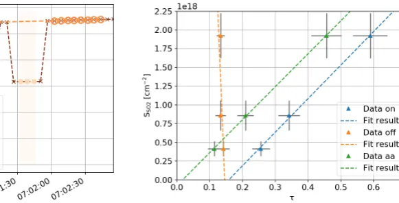
within the image plane. The calibration data is stored within instances of theDoasCalibDataclass, which is also used to retrieve the calibration curve. The latter is done by fitting a polynomial of appropriate order to the calibration data. Optionally, the fit can be performed using a weighted regression, to account for statistical uncertainties in the DOAS SO2-CDs (e.g. fit-errors, cf. Figure6).DoasCalibData objects can be stored using the FITS standard (including the FOV mask).
205
Figure 6.DOAS calibration curves - Plot showing example DOAS calibration data corresponding to the two different FOV parametrisations shown in Figure7). The fit was performed using a first-order weighted polynomial fit. The weights where calculated using the relative errors∆SSO2/ SSO2of the DOAS SO2-CDs. The y-axis offset is likely due to uncertainties in the DOAS retrieval (e.g. due to O3 interference) and is compensated by the calibration.
1 Note:Pypliscannot perform the DOAS analysis, the SO
2-CDs need to be retrieved using suitable 3rdparty software, e.g.
Note that the DOAS calibration curve is only valid within the image pixel area covered by the DOAS FOV. This is due to cross-detector variations in the SO2sensitivity (see Sect.2.2) and can be
corrected for using a mask retrieved from a cell calibration dataset. The mask is determined by fitting a 2D polynomial to a cell AA image (see prev. Sect.3.4.1) which is then normalised to the centre-position 210
of the DOAS FOV (illustrated in ex. script 7).
3.4.3. DOAS FOV search
Pyplisincludes two routines to retrieve the DOAS FOV mask (included in theDoasFOVEngineclass) based on a stack of AA images and a DOAS data vector:
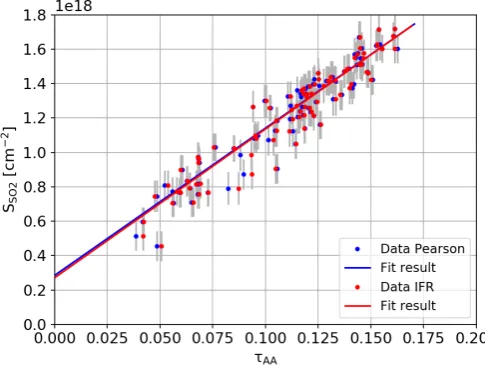
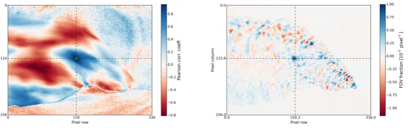
1. Pearson routine: this method loops over all image pixels in the AA stack and determines the 215
Pearson correlation coefficient between the corresponding AA time-series (τAA(t)) and the DOAS SO2-CD vector (SSO2(t)). The method yields a correlation image as shown in Figure7a, from
which the pixel coordinate with highest correlation (i0,j0) is extracted (see also [18]). Assuming a
circular FOV shape, the pixel extend of the FOV is estimated aroundi0,j0, by iteratively searching the disk radius with highest correlation between the AA and the DOAS time-series.
220
2. IFR routine: this method is based on [25] and uses an inversion algorithm to retrieve the FOV. Position and shape of the FOV is parametrised by fitting a 2D Super-Gaussian to the retrieved FOV distribution (shown in Figure7b, see AppendixC.2for details).
(a)Pearson method (b)IFR method
Figure 7.DOAS FOV search - DOAS FOV search results using (a), thePearsonand (b), theIFRmethod. The Pearson method (a) yields a FOV centered ati=159,j=124 and a disk radius of 4 pixels. For the IFR retrieval (b) a tolerance factor ofλ=2·10−3was chosen and a Super-Gaussian (without tilt) was fitted to the correlation image yielding a FOV centered ati=159.3,j=123.8,σ=7.1, asymmetry parametera =1.9 and a shape parameter ofb = 0.3 (for details see Eq. A2). The retrieved FOV positions show good agreement. Note, that the FOV was retrieved from downscaled images (Gauss pyramid level 2).
The retrieved FOV information (position, shape, convolution mask) is represented by theDoasFOV class and can be stored as FITS file.
225
3.5. Plume velocity analysis
Plume velocities can be retrieved either using the ICA cross-correlation method or using an optical flow algorithm. Both methods yield displacement estimates in units of pixels / time. These are converted into plume gas velocities based on the measurement geometry (MeasGeometry, see Sect.3.1). The relevant code is implemented in theplumespeed.pymodule.
3.5.1. Velocity retrieval using the ICA cross-correlation method
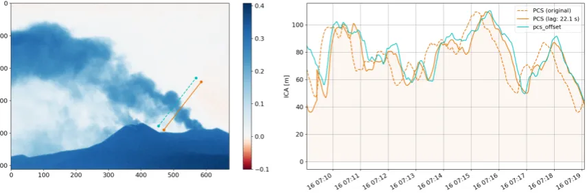
For the cross-correlation method, ICA time-series (see Eq.4) are determined using two PCS lines located at different positions downwind the emission source. Ideally, the PCS lines should be parallel and should cover an entire plume cross-section (indicated in Figure8, left). In a first step, the two time-series are re-sampled onto a regular grid (default is 1 s resolution). In a second step, a correlation 235
analysis is applied to the re-sampled data vectors in order to find the time lag corresponding to the highest correlation between both signals2. The method yields one average velocity vector, which is representative for the used image region and time-series. Note that the method intrinsically assumes, that the average plume propagation direction ¯ϕin thei,j-plane is aligned with the PCS normal (i.e.
¯
ϕ k n). Figureˆ 8shows results from an example cross-correlation analysis, resulting in a plume velocity
240
of 3.5 m/s.
Figure 8.Plume velocity retrieval using cross-correlation method. Left: example on-band OD image and the two used PCS lines. Right: ICA time-series for both lines (orange dashed and cyan line) and the PCS signal shifted using the retrieved correlation lag of 22.1 s (orange profile). The analysis yields an average gas velocity of 3.5 m/s.
3.5.2. Optical flow based velocity retrievals
Optical flow velocity retrievals are performed using the Farnebäck algorithm ([33]) which is implemented in the OpenCV library ([34]). The algorithm can estimate motion at the pixel-level by tracking local contrast features between consecutive frames. Note, however, that optical flow 245
algorithms may fail to detect motion in extended homogeneous image areas. In this case, appropriate corrections may be required (e.g. [35]).
All relevant calculations for optical flow based velocity retrievals are performed within the OptflowFarnebackclass. The class includes the Farnebäck algorithm itself as well as several pre and post-analysis routines. The latter include a routine that can detect and correct for unphysical motion 250
estimates in homogeneous image regions based on the method proposed by [35]. The correction identifies the local average velocity vector using peaks in histograms of an optical flow motion field.
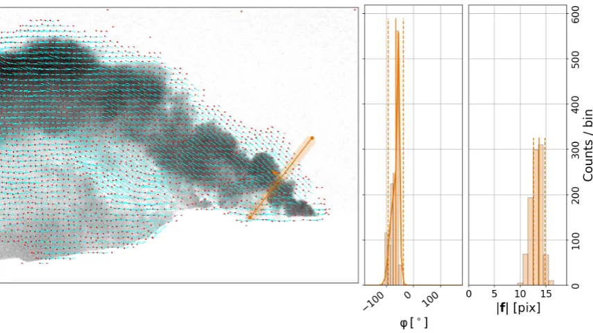
The Farnebäck algorithm itself requires specification of several input parameters (see e.g. OpenCV documentation). ThePyplisdefault settings follow the suggestions of [20]. An example flow field is shown in Figure9including results from the histogram post analysis within a narrow ROI around 255
an example retrieval line. The latter yield an average velocity magnitude of 4.2(±0.4)m/s and a predominant movement direction ofϕ=−65(±14)◦within the image plane. Optical flow plume
2 Note that the cross-correlation method is based on the fundamental assumption, that SO
2is conserved between the two PCS
Figure 9. Plume velocity optical flow - Example output of the Farnebäck optical flow algorithm including histograms of the flow vector orientation anglesϕ(middle) and magnitudes|f|(right) within an example ROI around the indicated PCS line (orange). From the latter, a plume velocity of 4.2(±0.4)m/s and a predominant movement direction ofθ=−65(±14)◦was retrieved using first and second moments of the displayed histogram distributions.
velocity retrievals, including the histogram post analysis method, are introduced in ex. script 9 (see TableA1).
3.6. Image based signal dilution correction 260
A correction for the signal dilution effect (see Sect.2.4) can be performed using theDilutionCorr class. The method is based on [19] and uses the model function
Imeas(λ) =I0(λ)e−e(λ)d+IA(λ)(1−e−e(λ)d) (5)
to retrieve atmospheric extinction coefficientsein the on and off-band regime. Here,Imeasare
measured intensities of dark terrain features within the images,dis the distance to these features andI0their initial intensity. The ambient intensityIAcan be approximated using gas free sky areas 265
in the plume images ([19]). For the retrieval, a set of measured intensities Imeas is extracted from vignetting corrected plume images using suitable terrain features (e.g. pixels along a volcanic flank). These intensities are fitted to Eq.5(as a function of their distanced) in order to retrieve the extinction coefficients in both wavelength regimes. The required distancesdto the features can be retrieved automatically, based on intersections of individual pixel viewing directions with the local topography 270
(using the Geonum library, for details see AppendixA).
The plume images can then be corrected for the signal dilution effect using the retrieved extinction coefficients (see Eq. 4 in [19]). The correction is only applied to plume pixels (e.g. using a
τAAthreshold mask). The required plume distances can be retrieved from the measurement geometry (for details see Sect.3.1).
275
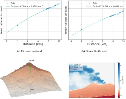
(a)Fit result on-band (b)Fit result off-band
(c)3D map distance retrieval (d)Corrected SO2-CD image
Figure 10.Signal dilution correction - (a) and (b) show the fit result of an example dilution analysis for the on and off-band regime, respectively. (c) shows a 3D map of the camera scene and (d) a dilution corrected SO2-CD image. The terrain features used for the dilution analysis are indicated in (c) and (d) (blue and lime coloured lines). (d) further includes the image region used to estimate the ambient intensityIA(blue rectangle) and an example PCS line used to compare emission-rates before and after the correction.
andeoff =0.0654 km−1(Figure10b) were retrieved using the two topographic profile lines shown
in Figure10cand10d. The correction yields an emission-rate of 4.8(±1.2)kg/s using the PCS line 280
shown in Figure 10d. The emission-rate of the uncorrected image is 1.6(±0.8)kg/s, corresponding to an underestimation of approximately 67 % at an average plume distance of 10.4(±0.1)km.
3.7. Emission-rate retrieval
Emission-rates can be determined using theEmissionRateAnalysisclass. The analysis is performed based on an image list containing calibrated SO2-CD images (see also AppendixD.2) and a specification 285
of one or more retrieval PCS lines (LineOnImageobjects, cf. Figure2). Plume velocities can be provided by the user (e.g. using the result of a cross-correlation analysis, see Sect. 3.5.1) or can be retrieved automatically during the emission-rate analysis using the Farnebäck optical flow routine (see Sect.
3.5.2). For the latter, three options are available:
1. flow_raw→the raw output of the Farnebäck algorithm is used. This should only be done if it 290
2. flow_histo → performs the histogram post-analysis proposed by [35] (cf. Sect. 3.5.2). The retrieved local average velocity vector for each PCS line is then used as a velocity estimate for the corresponding retrieval line.
295
3. flow_hybrid→reliable motion vectors from the flow field are used while unreliable ones are identified and replaced based on the histogram post-analysis (see prev. point).
Figure 11. Emission-rate retrieval - Emission-rates (top) and plume velocities (bottom) of the Etna example dataset on 16 September 2015 between 07:06 – 07:22 UTC using the retrieval line “PCS” shown in Figure8. The analysis was performed using 1.) a global velocity of 3.5 m/s (cyan, velo: glob, from the cross-correlation analysis), 2.) the raw output of the Farnebäck algorithm (thin orange) and 3.) using theflow_hybridmethod (bold orange). The retrieved effective velocities are plotted in the lower panel and correspond to the average velocities along the PCS line using theflow_hybridmethod. Uncertainties are displayed as shaded areas.
Figure11 shows results from an emission-rate analysis for the Etna test data (upper panel) including plume velocities retrieved using theflow_hybridmethod (lower panel). The AA images were calculated from dilution corrected on and off-band plume images using background modelling mode 300
6 (cf. Sect.3.3) and were corrected for cross-detector sensitivity variations using a mask retrieved from cell“a53"(cf. Figure5a). The AA images were calibrated using thePearsonDOAS calibration curve shown in Figure6.
4. Conclusions 305
In this paper the software packagePypliswas introduced.Pypliscontains an extensive collection of relevant algorithms for the analysis of UV SO2 camera data, particularly for the retrieval of
emission-rates from SO2-emitters (e.g. volcanoes, power plants, ships).
Apart from established analysis methods, such as cross-correlation based velocity retrievals (e.g. [26]) or cell and DOAS calibration (e.g. [18]),Pyplisincorporates more recent developments. These 310
include an implementation of the DOAS FOV retrieval algorithm proposed by [25], a routine to correct for the signal dilution effect based on [19], or pixel based gas velocity retrievals using an optical flow algorithm (e.g. [20]). The latter incorporates a method to detect and correct for ill-constraint optical flow motion-vectors based on [35]. Furthermore,Pyplisincludes a framework to perform a detailed 3D-analysis of the observed camera scene including automatic online access to high resolution 315
Due to this extensive collection of algorithms,Pyplisprovides flexibility with regard to the analysis 320
strategy and is highly adaptable to different data situations. The object oriented architecture of the API gives intuitive access to the main features and makes it easy to compare individual methods (e.g. different plume velocity retrievals, as illustrated in this paper).Pyplisis open-source and can be operated both on Windows and Unix machines. Thus, it is well suited for inter-comparison studies, the exchange of analysis results or for the development and verification of new methods.
325
ThePyplisinstallation includes numerous example scripts which were used in this paper to introduce the main features of the software. The examples are based on a 15 min dataset recorded at Mt. Etna, Italy in September 2015 which is freely available and can be downloaded from the website. Finally, the authors wish to point out thatPyplismay also be used for other applications based on the same measurement principle (e.g. NO2cameras) and that parts of it can also be useful for other 330
remote sensing applications (e.g. the engine for geometrical calculations). ThePyplissoftware is hosted on GitHub:https://github.com/jgliss/pyplis. The code documentation and further information (e.g. installation instructions) can be found on the documentation website:http://pyplis.readthedocs.io.
Acknowledgments: The authors like to thank theAtmosphere and Remote Sensinggroup from the Institute of Environmental Physics in Heidelberg, Germany for providing image data for test purposes and for collaboration 335
during the Etna field campaign in 2015. The work of K.S., A.K. and A.S.D. was partly supported by the European Research Council (ERC) under the European Union’s Horizon 2020 research and innovation programme under grant agreement No 670462 (COMTESSA). J.G. wishes to thank T. Skauli, M. Vogt, and A. Donath for helpful discussions related to the development of the software and the drafting of the manuscript.
Author Contributions: J.G. designed, developed and tested the software including the example scripts and 340
wrote the manuscript. K.S., A.S.D., A.K, H.S. and A.S. contributed to the API design (selection of implemented methods / algorithms) and helped testing and debugging the code. H.S. provided the IFR algorithm and wrote the corresponding part in the paper.
Conflicts of Interest:The authors declare no conflict of interest.
Abbreviations 345
The following abbreviations are used in this manuscript:
UV Ultraviolet CD Column density
DOAS Differential optical absorption spectroscopy FOV Field of view
OD Optical density
AA SO2apparent absorbance PCS Plume cross section ICA Integrated column amount
API Application programming interface IFR In-operation field-of-view retrieval
Appendix A. The Geonum Python library
ThePyplisclassMeasGeometry(see Sect.3.1) makes use of the Python library Geonum [31]. Geonum
350
was developed by J. Gliss in parallel toPyplisand features vector based geographical calculations in three dimensions as well as access and handling of high resolution topographic data. It supports topographic data based on the Etopo1 global relief model ([36]) and from the NASA shuttle radar topography mission (SRTM, [37]). The latter can be accessed and downloaded automatically within Geonum from the SRTM online database (for details see information on the Geonum [31] website). 355
Appendix A.1. Pixel based retrieval of distances to local terrain features
azimuth and elevation angle) with the local topography. This is particularly helpful for the image 360
based correction of the signal dilution effect (see Sect.3.6and Figure10).
Appendix B. Dark and offset correction
Pyplisincludes two options to perform dark and offset corrections for image data. Both methods require access to the exposure time of the images (e.g. from the image file names, see also AppendixE).
1. Option 1: Modelling of dark / offset image
The correction is performed based on two dark images, one being recorded at short(est) exposure time (offset signalO) and the second one at long(est) exposure time (dark current + offset signal,
D). A dark image is then calculated based on the exposure time of the input imageIusing the following formula:
Dmod=O+
(D−O)∗texp,I (texp,D−texp,O)
. (A1)
This mode is, for instance, used for the Envicam-2 camera type (see Appendix E.2). The 365
corresponding methodmodel_dark_imageis part of theprocessing.pymodule. 2. Option 2: Subtraction of dark image
Dark and offset correction is performed by subtracting a single dark imageD(containing dark and offset) which thus, needs to be recorded at the same camera exposure time. This mode is for 370
instance used for the HD-Custom camera (see AppendixE.2).
The detector dark current depends on the temperature. In case of temperature variations it is therefore recommended to use dark images recorded close in time to a given plume image.
Appendix C. Spectrometer FOV search: additional information
Appendix C.1. Temporal merging of image and DOAS data 375
TheImgStackclass includes three methods to merge a set of camera images (stacked within such anImgStack) and a DOAS time series vector, both sampled on arbitrary irregular grids.
• First method: averaging of camera images
This method averages all images in the stack based on start / stop time stamps of the 380
spectrometer data (i.e. the image sampling rate should be larger than the spectrum sampling rate). Spectra for which no image data could be found are removed.
• Second method: vice versa interpolation of both grids
This method uses the unified sampling grid (all time stamps from both datasets) and performs 385
interpolation of the DOAS data vector (at image acquisition time stamps) and vice versa. The method is slow compared to method 1 since each image pixel of the stack is interpolated. However, it results in more data points, which can be an advantage especially for short time series. This method can be significantly accelerated by reducing the image size or by only performing the analysis within a certain image region (c.f. example script no. 6, TableA1, script 390
option: DO_FINE_SEARCH). The time series interpolation is done using thepandasPython library.
• Third method: nearest data point
This method loops over all spectra and for each spectrum, finds the image which is nearest in 395
Appendix C.2. FOV determination applying the IFR method
The In-operation Field of view Retrieval (IFR) method is an implementation of the method proposed by [25]. IFR applies a linear camera model to invert the FOV of a low-resolution instrument 400
(in this case a DOAS spectrometer) from imager data without a-priori information (e. g. FOV position, size and shape). The inversion problem is typically under-determined for SO2camera applications.
Therefore, the iterative LSMR method ([38]) is applied to retrieve the FOV coefficients depending on the regularisation parameterλ.
The choice ofλis somewhat arbitrary, but may influence the IFR results depending on the input
405
data quality. The default value isλ= 10−6. However, in case only a small sample size is available, λmay need to be increased (e. g. λ= 10−3) in order to produce meaningful results. A side effect of
increasingλis a spatial smoothing of the results potentially leading to unrealistic large FOVs. Figure7b
shows a sample FOV distribution retrieved from the Etna test data (88 images) usingλ = 2·10−3.
In order to reach the final goal of gaining a calibration curve from the image stack containing 410
AA images, individual images need to be convolved with the FOV of the low-resolution instrument. Therefore, a parametrised FOV is fitted to the IFR results, which is more applicable to ground-based instruments than the parametrisation proposed by [25]. We propose the following elliptical Super-Gaussian FOV parametrisation g of the IFR result depending on pixel coordinates i,j in horizontal and vertical direction, respectively:
415
g(i,j) =C+Ae−
[i−im σ ]
2
+h(j−jmσ )ai2
b
(A2)
where,Cis a constant offset,Athe amplitude,xmandymdefine the centre position,σmeasures
the width inx-direction, the asymmetry parameterameasures the ratio of the semi-axes (e.g.a=1 yields an only circular FOV), andbis the shape parameter of the Super Gaussian (e.g.b=1 yields an only Gaussian FOV,b=10 approximates a flat-disk FOV).
420
If an additional tilt of the FOV is required in case of an elliptical FOV, the above fit may be performed in a transformed coordinate system.
i0 j0
!
= cosθ −sinθ
sinθ cosθ
!
i−im j−jm
!
(A3)
defines the transformation into tilted coordinatesi0andj0. Equation (A2) is then replaced by
g=C+Aexp − i0 σ 2 +
j0a
σ
2!b
. (A4)
Appendix D. Basic data structure
ThePypliscode hierarchy for the emission-rate analysis is shown in Figure2. The structure is based on the work flow shown in FigureA1and includes most of the relevant classes required for the emission-rate analysis.
Appendix D.1. Setup and Dataset classes 425
The most important classes related to data import and image management are:
• Setup classes (e.g. Camera, Source, MeasSetup), which can be used to specify all relevant meta information.
• Dataset classes (Dataset,CellCalibEngine), which can be used for automatic image separation, for instance by image type (e.g. on, off, dark, offset) or acquisition time.
Figure A1.Main analysis steps - Flowchart showing the main analysis steps for emission-rate retrievals (cf. Table1). The colours indicate geometrical calculations (yellow), background modelling (light gray), camera calibration (light blue), plume speed retrieval (light orange) and the central processing steps for the emission-rate retrieval (light green). Shaded and dashed symbols indicate optional or alternative analysis methods.
Appendix D.2. ImgList classes
Image list classes are central for the data analysis. They can be found in theimagelists.pymodule (e.g. ImgList,CellImgList). AnImgListtypically contains images of one specific type (e.g. on-band) corresponding to a certain time window. In order to avoid potential memory overflows, images are loaded, processed and unloaded successively withinImgListobjects. The most important features are
435
described in the following.
Linking ofImgListobjects
ImgListcan be linked to each other (e.g. off to on-band list). This means, that, whenever the list
index (i.e. the current image) is changed inImgListA(e.g. the on-band images), it is also changed in ImgListB(ifBis linked toA), such that the current image inBis closest in time to the one inA.
440
Image preparation and processing modes
Image lists include several image preparation options (e.g. size reduction, cropping, blurring). Further, if certain requirements are fulfilled, additional preparation options and routines can be activated:
• darkcorr_mode→images are automatically corrected for dark and offset. Requires a dark image 445
• tau_mode → if active, images are converted into τ images on image load (using the
PlumeBackgroundModelclass to retrieve the plume background intensities). Requires availability of a
sky reference image in the list (only for background modelling modes 1 - 6, see Sect.3.3). 450
• aa_mode→if active, images are converted intoτAAimages on image load. Requires an off-band
image list to be linked to the list and availability of a sky reference image in both lists (only for background modelling modes 1 - 6, see Sect.3.3).
• sensitivity_corr_mode→if active, images will be corrected for sensitivity variations due to shifts in the filter transmission windows (see Sect.2.2). Requires a corresponding correction mask to 455
be available in the list. The latter can for instance be retrieved from cell calibration data (see Sect.
3.4.1).
• calib_mode→images are loaded as calibrated SO2-CD images. Requires list to be inaa_modeand
calibration data to be available in the list. The latter can be of typeCellCalibDataorDoasCalibData (see Figure2). Warns ifsensitivity_corr_modeis inactive.
460
• optflow_mode→if active, the Farnebäck optical flow will be calculated between current and the next list image (using theOptflowFarnebackclass, see Sect.3.5.2).
• vigncorr_mode→if active, images will be corrected for vignetting. Requires availability of a vignetting mask in the list or a sky reference image from which the mask is determined.
All active image preparation options are applied on image load (i.e. whenever the current image is 465
changed in theImgList).
Appendix D.3. Processing classes
Most of the relevant processing classes are shown in Figure2. They include:
• MeasGeometry(geometry.py)→all relevant geometrical calculations (Sect.3.1).
• OptflowFarneback(plumespeed.py)→calculation and post analysis of optical flow field between two
470
images (Sect.3.5.2).
• CellCalibData(cellcalib.py)→pixel based retrieval of cell calibration polynomial (based on a set of cellτimages) and retrieval of sensitivity correction mask (Sect.3.4.1).
• DoasFovEngine(doascalib.py)→performs FOV search of DOAS spectrometer within camera images (Sects.3.4.2&C).
475
• DoasFov(doascalib.py)→DOAS FOV information such as position, shape, convolution mask (Sects.
3.4.2&C). Can be saved as FITS file.
• DoasCalibData(doascalib.py) →DOAS calibration data, i.e. vector of τand SO2-CD values for
fitting of calibration polynomial (Sect.3.4.2). Can be saved as FITS file.
• LineOnImage(processing.py)→data extraction (interpolation) along a line on a discrete 2D image
480
grid (e.g. SO2-CDs from calibrated images or displacement vectors from optical flow field, Sect.
3.7).
• EmissionRateAnalysis (fluxcalc.py) → Performs emission-rate analysis based on an ImgList containing calibrated images. Emission-rates can be retrieved along one (or more) plume cross section lines (LineOnImageobjects). Has several options related to the plume velocity retrieval (Sect.
485
3.7).
• EmissionRates (fluxcalc.py) → Contains results (time series) of an emission-rate analysis (i.e. including plume velocity data). Specific for one PCS line and one velocity retrieval (e.g. the analysis shown in Figure11creates 3EmissionRatesobjects for each of the 3 different velocity retrievals, Sect.3.7).
490
Further important classes (not shown in Figure2) are:
• PlumeBackgroundModel(plumebackground.py) →performsτ image modelling using either of the
available modelling modes (Sect.3.3).
• VeloCrossCorrEngine(plumespeed.py)→high level class to calculate the plume velocity using the cross-correlation method (Sect.3.5.1).
• DilutionCorr(dilutioncorr.py)→engine to perform signal dilution correction (Sect.3.6).
• ImgStack(processing.py) →contains a series of images (stored as 3D numpy array) as well as supplementary data (e.g. acq. time stamps, exposure times of all stacked images) and basic processing operations (time merging with other data, up / downscaling). Can be saved as FITS file.
500
Appendix E. Supplementary information and test data
Appendix E.1. Example dataset and example scripts
Most of the example and introduction scripts provided withPyplisare based on a short example dataset recorded at Mt. Etna, Italy on 16.09.2015, using a type Envicam-2 camera. It includes∼15 minutes of plume data (between 07:06 – 07:22 UTC, see e.g. Figure11.) as well as cell calibration data 505
including suitable background images (between 06:59 – 07:04 UTC, see Figure5). These data is used for demonstration purposes in the provided example scripts, which are summarised in TableA1. The data is not part of thePyplisinstallation and can be downloaded from the website.
Table A1.Pyplisexample scripts, sub-categorised into introductory scripts (0.1–0.7) and scripts related to the emission-rate analysis of the Etna test data (1–12)
No. Name Description Sect
0.1 ex0_1_img_handling.py TheImgclass - Image import and dark correction
3.2
0.2 ex0_2_camera_setup.py TheCameraclass - Definition of camera specifications and image file name convention
D
0.3 ex0_3_imglists_manually.py Introduction intoImgListobjects D.2 0.4 ex0_4_imglists_auto.py Automatic creation of ImgList objects
using the ECII defaultCameratype
D.2
0.5 ex0_5_optflow_livecam.py Interactive optical flow using web cam 3.5.2
0.6 ex0_6_pcs_lines.py Plume cross section lines (creation and orientation ofLineOnImageobjects)
3.7
0.7 ex0_7_cellcalib_manual.py Introduction into cell calibration and theCellCalibDataobject (manually)
3.4.1
1 ex01_analysis_setup.py Create MeasSetup class and initiate analysis Dataset object from that (see Figure2)
3.4.1
2 ex02_meas_geometry.py Introduction into theMeasGeometryclass 3.1
3 ex03_plume_background.py The PlumeBackgroundModel class
-background modelling and τ image
retrieval
3.3
4 ex04_prep_aa_imglist.py Preparation of image list containing AA images
D.2
5 ex05_cell_calib_auto.py Automatic cell calibration using the CellCalibEngineclass
3.4.1
6 ex06_doas_calib.py DOAS calibration and FOV search 3.4.2
7 ex07_doas_cell_calib.py Retrieval of AA sensitivity correction mask
3.4
8 ex08_velo_crosscorr.py Plume velocity retrieval using
cross-correlation
9 ex09_velo_optflow.py Plume velocity retrieval using Farnebäck optical flow algorithm usingOptflowFarnebackclass
3.5.2
10 ex10_bg_imglists.py Retrieval of background image lists (on, off) usingDatasetclass
D
11 ex11_signal_dilution.py Correction for signal dilution and the DilutionCorrclass
3.6
12 ex12_emission_rate.py Emission-rate retrieval for the test dataset
3.7
SETTINGS.py Global settings for example scripts
Appendix E.2. Camera specifications
In order to use all features ofPyplis(e.g. automatic file separation, automatic dark and offset 510
correction, geometrical calculations), certain camera characteristics need to be provided by the user. These information is typically specified within aCameraclass (setupclasses.pymodule). The required information includes specifications about the image sensor (e.g. pixel geometry) and optics (e.g. focal length) as well as file naming conventions (e.g. how to retrieve the filter type or the image acquisition time from file names).Pyplisprovides the possibility to define new default camera types which store 515
all relevant camera information to thePyplisdata filecam_info.txt, which can be found in thedata
directory of the installation (see ex. script 0.2 for details).
Appendix E.3. Source specifications
Default source information (e.g. longitude, latitude, altitude) can be specified in the file
my_sources.txtin the installationdatadirectory. 520
References
1. Robock, A. Volcanic eruptions and climate. Reviews of Geophysics2000,38, 191–219.
2. IPCC.Climate Change 2013: The Physical Science Basis. Contribution of Working Group I to the Fifth Assessment Report of the Intergovernmental Panel on Climate Change; Cambridge University Press: Cambridge, United Kingdom and New York, NY, USA, 2013; p. 1535.
525
3. Carroll, M.R.; Holloway, J.R.Volatiles in magmas; Mineralogical Society of America, 1994. Last access: 30 July 2017.
4. Oppenheimer, C.; Fischer, T.; Scaillet, B. 4.4 - Volcanic Degassing: Process and Impact. InTreatise on Geochemistry (Second Edition); Elsevier, 2014; pp. 111–179.
5. Lübcke, P.; Bobrowski, N.; Arellano, S.; Galle, B.; Garzón, G.; Vogel, L.; Platt, U. BrO / SO2molar ratios 530
from scanning DOAS measurements in the NOVAC network. Solid Earth2014,5, 409–424.
6. Bobrowski, N.; von Glasow, R.; Giuffrida, G.B.; Tedesco, D.; Aiuppa, A.; Yalire, M.; Arellano, S.; Johansson, M.; Galle, B. Gas emission strength and evolution of the molar ratio of BrO / SO2 in the plume of Nyiragongo in comparison to Etna. Journal of Geophysical Research: Atmospheres2015, 120, 277–291. 2013JD021069.
535
7. Moffat, A.J.; Millan, M.M. The applications of optical correlation techniques to the remote sensing of SO2 plumes using sky light.Atmospheric Environment (1967)1971,5, 677–690.
8. Platt, U.; Stutz, J.Differential Optical Absorption Spectroscopy: Principles and Application; Springer, 2008. 9. Platt, U.; Perner, D. Direct measurements of atmospheric CH2O, HNO2, O3, NO2, and SO2by differential
optical absorption in the near UV.J. Geophys. Res.1980,85, 7453–7458. 540
10. Galle, B.; Johansson, M.; Rivera, C.; Zhang, Y.; Kihlman, M.; Kern, C.; Lehmann, T.; Platt, U.; Arellano, S.; Hidalgo, S. Network for Observation of Volcanic and Atmospheric Change (NOVAC) - A global network for volcanic gas monitoring: Network layout and instrument description. J. Geophys. Res.2010,115. 11. Mori, T.; Burton, M. The SO2camera: A simple, fast and cheap method for ground-based imaging of SO2
12. Bluth, G.; Shannon, J.; Watson, I.; Prata, A.; Realmuto, V. Development of an ultra-violet digital camera for volcanic SO2imaging.Journal of Volcanology and Geothermal Research2007,161, 47 – 56.
13. Kantzas, E.P.; McGonigle, A.; Tamburello, G.; Aiuppa, A.; Bryant, R.G. Protocols for UV camera volcanic SO2 measurements.Journal of Volcanology and Geothermal Research2010,194, 55 – 60.
14. Stebel, K.; Amigo, A.; Thomas, H.; Prata, A. First estimates of fumarolic SO2fluxes from Putana volcano, 550
Chile, using an ultraviolet imaging camera.Journal of Volcanology and Geothermal Research2015,300, 112–120. 15. D’Aleo, R.; Bitetto, M.; Delle Donne, D.; Tamburello, G.; Battaglia, A.; Coltelli, M.; Patanè, D.; Prestifilippo, M.; Sciotto, M.; Aiuppa, A. Spatially resolved SO2flux emissions from Mt Etna. Geophys. Res. Lett.2016,
43, 7511–7519.
16. Tamburello, G.; Aiuppa, A.; McGonigle, A.J.S.; Allard, P.; Cannata, A.; Giudice, G.; Kantzas, E.P.; Pering, 555
T.D. Periodic volcanic degassing behavior: The Mount Etna example. Geophys. Res. Lett. 2013, 40, 4818–4822.
17. Kern, C.; Kick, F.; Lübcke, P.; Vogel, L.; Wöhrbach, M.; Platt, U. Theoretical description of functionality, applications, and limitations of SO2cameras for the remote sensing of volcanic plumes. Atmospheric
Measurement Techniques2010,3, 733–749. 560
18. Lübcke, P.; Bobrowski, N.; Illing, S.; Kern, C.; Alvarez Nieves, J.M.; Vogel, L.; Zielcke, J.; Delgado Granados, H.; Platt, U. On the absolute calibration of SO2 cameras. Atmospheric Measurement Techniques2013,
6, 677–696.
19. Campion, R.; Delgado-Granados, H.; Mori, T. Image-based correction of the light dilution effect for SO2 camera measurements. Journal of Volcanology and Geothermal Research2015,300, 48 – 57.
565
20. Peters, N.; Hoffmann, A.; Barnie, T.; Herzog, M.; Oppenheimer, C. Use of motion estimation algorithms for improved flux measurements using SO2cameras.Journal of Volcanology and Geothermal Research2015,
300, 58 –69.
21. Kern, C.; Lübcke, P.; Bobrowski, N.; Campion, R.; Mori, T.; Smekens, J.F.; Stebel, K.; Tamburello, G.; Burton, M.; Platt, U.; Prata, F. Intercomparison of SO2camera systems for imaging volcanic gas plumes.Journal of 570
Volcanology and Geothermal Research2015,300, 22–36.
22. Tamburello, G.; Kantzas, E.; McGonigle, A.; Aiuppa, A. Vulcamera: a program for measuring volcanic SO2 using UV cameras. Annals of Geophysics2011,54.
23. Peters, N. Plumetrack SO2flux calculator. https://ccpforge.cse.rl.ac.uk/gf/project/plumetrack/, 2014. (accessed: 11.09.2017).
575
24. Kern, C.; Sutton, J.; Elias, T.; Lee, L.; Kamibayashi, K.; Antolik, L.; Werner, C. An automated SO2camera system for continuous, real-time monitoring of gas emissions from K¯ılauea Volcano’s summit Overlook Crater. Journal of Volcanology and Geothermal Research2015,300, 81–94.
25. Sihler, H.; Lübcke, P.; Lang, R.; Beirle, S.; de Graaf, M.; Hörmann, C.; Lampel, J.; Penning de Vries, M.; Remmers, J.; Trollope, E.; Wang, Y.; Wagner, T. In-operation field-of-view retrieval (IFR) for satellite and 580
ground-based DOAS-type instruments applying coincident high-resolution imager data. Atmospheric Measurement Techniques2017,10, 881–903.
26. McGonigle, A.J.S.; Hilton, D.R.; Fischer, T.P.; Oppenheimer, C. Plume velocity determination for volcanic SO2flux measurements.Geophysical Research Letters2005,32. L11302.
27. Klein, A.; Lübcke, P.; Bobrowski, N.; Kuhn, J.; Platt, U. Plume propagation direction determination with 585
SO2cameras. Atmospheric Measurement Techniques2017,10, 979–987.
28. Kern, C.; Deutschmann, T.; Vogel, L.; Wöhrbach, M.; Wagner, T.; Platt, U. Radiative transfer corrections for accurate spectroscopic measurements of volcanic gas emissions. B. Volcanol.2010,72, 233–247.
29. Kern, C.; Deutschmann, T.; Werner, C.; Sutton, A.J.; Elias, T.; Kelly, P.J. Improving the accuracy of SO2 column densities and emission rates obtained from upward-looking UV-spectroscopic measurements 590
of volcanic plumes by taking realistic radiative transfer into account. Journal of Geophysical Research: Atmospheres2012,117.
30. Vogel, L.; Galle, B.; Kern, C.; Delgado Granados, H.; Conde, V.; Norman, P.; Arellano, S.; Landgren, O.; Lübcke, P.; Alvarez Nieves, J.M.; Cárdenas Gonzáles, L.; Platt, U. Early in-flight detection of SO2 via Differential Optical Absorption Spectroscopy: a feasible aviation safety measure to prevent potential 595
33. Farnebäck, G., Two-Frame Motion Estimation Based on Polynomial Expansion. InImage Analysis: 13th Scandinavian Conference, SCIA 2003 Halmstad, Sweden, June 29 – July 2, 2003 Proceedings; Springer Berlin 600
Heidelberg: Berlin, Heidelberg, 2003; pp. 363–370.
34. Bradski, G. The OpenCV Library. Dr. Dobb’s Journal of Software Tools2000.
35. Gliß, J.; Stebel, K.; Kylling, A.; Sudbø, A. Optical flow gas velocity analysis in plumes using UV cameras – Implications for SO2-emission-rate retrievals investigated at Mt. Etna, Italy, and Guallatiri, Chile.
Atmospheric Measurement Techniques Discussions2017,2017, 1–30. 605
36. Amante, C.; Eakins, B.W. ETOPO1 Global Relief Model converted to PanMap layer format, 2009. 37. Farr, T.G.; Rosen, P.A.; Caro, E.; Crippen, R.; Duren, R.; Hensley, S.; Kobrick, M.; Paller, M.; Rodriguez, E.;
Roth, L.; Seal, D.; Shaffer, S.; Shimada, J.; Umland, J.; Werner, M.; Oskin, M.; Burbank, D.; Alsdorf, D. The Shuttle Radar Topography Mission. Rev. Geophys.2007,45.
38. Fong, D.C.L.; Saunders, M. LSMR: An Iterative Algorithm for Sparse Least-Squares Problems. SIAM 610
Journal on Scientific Computing2011,33, 2950–2971.