Telephone: +44 (0)1582 763133 Web: http://www.rothamsted.ac.uk/
Rothamsted Research is a Company Limited by Guarantee Registered Office: as above. Registered in England No. 2393175. Registered Charity No. 802038. VAT No. 197 4201 51. Founded in 1843 by John Bennet Lawes.
Rothamsted Repository Download
A - Papers appearing in refereed journals
Sadeghi-Tehran, P., Angelov, P., Virlet, N. and Hawkesford, M. J. 2019.
Scalable Database Indexing and Fast Image Retrieval Based on Deep
Learning and Hierarchically Nested Structure Applied to Remote Sensing
and Plant Biology. Journal of Imaging. 5 (33).
The publisher's version can be accessed at:
•
https://dx.doi.org/10.3390/jimaging5030033
The output can be accessed at:
https://repository.rothamsted.ac.uk/item/8w992
.
© 1 March 2019, Rothamsted Research. Licensed under the Creative Commons CC BY.
Journal of
Imaging
Article
Scalable Database Indexing and Fast Image Retrieval
Based on Deep Learning and Hierarchically Nested
Structure Applied to Remote Sensing and
Plant Biology
Pouria Sadeghi-Tehran1,* , Plamen Angelov2 , Nicolas Virlet1and Malcolm J. Hawkesford1
1 Department of Plant Sciences, Rothamsted Research, Harpenden AL5 2JQ, UK;
[email protected] (N.V.); [email protected] (M.J.H.)
2 School of Computing and Communications, InfoLab21, Lancaster University, Lancaster LA1 4WA, UK;
* Correspondence: [email protected]
Received: 6 November 2018; Accepted: 18 February 2019; Published: 1 March 2019
Abstract: Digitalisation has opened a wealth of new data opportunities by revolutionizing how images are captured. Although the cost of data generation is no longer a major concern, the data management and processing have become a bottleneck. Any successful visual trait system requires automated data structuring and a data retrieval model to manage, search, and retrieve unstructured and complex image data. This paper investigates a highly scalable and computationally efficient image retrieval system for real-time content-based searching through large-scale image repositories in the domain of remote sensing and plant biology. Images are processed independently without considering any relevant context between sub-sets of images. We utilize a deep Convolutional Neural Network (CNN) model as a feature extractor to derive deep feature representations from the imaging data. In addition, we propose an effective scheme to optimize data structure that can facilitate faster querying at search time based on the hierarchically nested structure and recursive similarity measurements. A thorough series of tests were carried out for plant identification and high-resolution remote sensing data to evaluate the accuracy and the computational efficiency of the proposed approach against other content-based image retrieval (CBIR) techniques, such as the bag of visual words (BOVW) and multiple feature fusion techniques. The results demonstrate that the proposed scheme is effective and considerably faster than conventional indexing structures.
Keywords:content-based image retrieval; deep convolutional neural networks; information retrieval; data indexing; recursive similarity measurement; deep learning; bag of visual words; remote sensing
1. Introduction
Today, digital images and videos are ubiquitous in every domain. The advancement in
multi-media technologies has led to the generation of an enormous number of images and videos. The size of image repositories has increased rapidly in many domains, such as biology, remote sensing, medical, military, and web-searching. The use of automated data acquisition systems, such as modern
phenotyping platforms [1–3] has revolutionized the way the data is collected and analyzed. The plant
science community is seeking novel solutions to fully exploit all the potential offered by such new platforms equipped with high-resolution remote sensing sensors. Any large-scale dataset in modern biological sciences first and foremost requires reliable data infrastructure and an efficient information retrieval system. For image repositories of large scale, manual tagging is infeasible and is prone to errors, due to users’ subjective opinions. Thus, to utilize such unstructured and complex image
collections, there is a substantial need for content-based image retrieval (CBIR) systems for browsing through images at a large scale and to classify, structure, and retrieve relevant information requested by the users.
Information retrieval (IR) refers to finding material (image repositories or documents) of an
unstructured nature (image or text) that satisfies an information need from within large collections [4].
There is a fundamental difference between CBIR and search by text and metadata. Searching methods based on metadata rarely examine the content of an image itself but rather rely on manual annotations and tagging. In these systems, words are stored as ASCII character strings to describe image content. However, the high complexity of images cannot be described easily by keywords; thus, retrieval systems which are based solely on manual annotation often lead to unsatisfactory outcomes. In contrast, CBIR does not require keywords (manual annotation) and desired images are retrieved automatically based on their similarity to the query representation [5–7].
Although CBIR techniques are beginning to find a foothold in many applications, such as biology, remote sensing, satellite imaging, etc., the technology still suffers from lack of maturity due to a significant gap towards semantic-aware retrieval from visual content. A major challenge associated with CBIR systems is to extract information from an image which is unique and representative,
to overcome the issue of so calledsemantic-gap. Thesemantic-gaprefers to low-level features of images
such as colors and texture, but those features might not be able to extract a higher level of understanding
of the image perceived by humans [8]. Due to the absence of solid evidence on the effectiveness of
CBIR techniques for high-throughput datasets with varied collections of images, opinion is still sharply divided regarding the reliability and performance of such systems in real-time. It is essential to standardize CBIR for easy access to data and speed up the retrieval process.
In this paper, a new concept of CBIR is employed to exploit the opportunities presented by large image-based repositories, particularly in remote sensing and plant biology. The proposed approach, which relies solely on the contents of the images, will pave the way for a computationally efficient and real-time image querying through an unstructured image database. An end-to-end CBIR framework is conducted without supervision. First, we utilize a deep CNN model as a feature extractor to obtain the feature representations from the activations of the convolutional layers. In the next step, a hierarchically nested database indexing structure and local recursive density estimation are developed to facilitate an efficient and fast retrieval process. Finally, the key elements of CBIR, accuracy and computational efficiency, are evaluated and compared with the state-of-the-art CBIR techniques.
2. Related Works
The core modules of any CBIR systems include image representation, database indexing, and image scoring, described as detailed below:
2.1. Image Representation
At the core, visual features affect every aspect of computer vision applications, including CBIR. The success of any CBIR system crucially depends on the feature representation of the images extracted by applying an image descriptor. Although over the past decades a variety of feature extraction techniques have been developed to find semantically richer image representations, it still remains one of the key challenges in CBIR applications.
2.1.1. Hand-crafted Feature Extraction Techniques
J. Imaging2019,5, 33 3 of 21
• Color properties are extracted directly from the pixel densities over the whole image, segmented
regions/bins, or sub-image. Image descriptors that characterize the color properties of an image seek to model the distribution of the pixel intensities in each channel of the image. These methods include color statistics, such as deviation, mean, and skewness, along with color histograms. Since color features are robust to background complications and are invariant to the size or orientation of an image, the color based methods have become one of the most common techniques in CBIR [9–11].
• Texture properties measure visual patterns in images that contain important information about
the structural arrangement of surface i.e., fabric, bricks, etc. Texture descriptors seek to model the feel, appearance, and overall tactile quality of an object in an image and are defined as a structure of surfaces formed by repeating a particular element or several elements in different relative spatial distribution and synthetic structure. In general, the repetition involves local variations of scale, orientation, or other geometric and optical features of the elements [12,13].
• Shape properties can also be considered as one of the fundamental perceptual characteristics.
Shape properties take on many non-geometric and geometric forms, such as moment invariants, aspect ratio, circularity, and boundary segments. There are difficulties associated with shape representation and descriptors techniques due to noise, occlusion, and arbitrary distortion, which often causes inaccuracies in extracting shape features. Nonetheless, the method has shown promising results to describe the image content [14,15].
Whilst the above techniques focus on primitive features, more recent techniques have been aimed to find semantically richer image representations by extracting a collection of local invariant features. The main advantage of semantic features is locality, which means that the extracted features are local and robust to clutter and occlusion. Also, individual features can be matched to a large database of objects and have close to real-time performance.
One of the most effective techniques is the bag of visual words technique [16,17]. The main reasons that BOVW has gained popularity in classification and retrieval applications are the use of powerful
local descriptors, such as Scale Invariant Feature Transform (SIFT) [18], Speeded Up Robust Features
(SURF) [19], and Binary Robust Invariant Scalable Keypoints (BRISK) [20]. In addition, the vector
representations can be compared with standard distances, and subsequently be used for effective CBIR. However, the main drawback of BOVW is the high dimensional vector representing an image. Although a high-dimensional vector usually provides better exhaustive search results compared to a low-dimensional one, it is more difficult to index efficiently. Aggregated vectors, such as Fisher Vector
(FV) [21] and Vector of Locally Aggregated Descriptors (VLAD) [22] aim to address this problem by
encoding an image into a single vector, reducing the dimensionality without noticeably impacting the accuracy [16,17].
Nevertheless, despite the robustness of local descriptors techniques, global features are still desirable in a variety of computer vision applications. Ultimately, having an intimate knowledge of the dataset contents will provide a better perspective for which feature extraction techniques might be appropriate. For example, datasets that have relatively different color distributions, color descriptors will be more effective. Nonetheless, the effectiveness of hand-crafted feature representation in CBIR is inherently limited, as these approaches mainly operate at the primitive level. As presented in the following section, higher accuracy will be achieved by extracting semantic features from images based on learning-based features using deep networks.
2.1.2. Learning-based Features Using Deep Convolutional Neural Network
Recent years have witnessed the success of learning based features using Deep Neural Networks
(DNNs) [23–25]. Unlike conventional global and local feature extraction methods, which often use
shallow architecture and solely rely on human-crafted features, deep Conventional Neural Networks
are considered the most well-known architecture for visual analysis [26]. CNN models attempt to
non-linear transformations [27]. In CNNs, features are extracted at multiple levels of abstracts and allow the system to learn complex functions that directly map raw sensory input data to the output, without relying on hand-engineered features using domain knowledge.
CNN has achieved state-of-the-art performance in a variety of applications, including natural
language processing [28,29], speech recognition [30], and object recognition [31]. Inspired by the
success of CNN in many computer vision applications, it has started to gain a foothold in the research area of CBIR. Subsequently, CNN models have been proposed to improve the image
retrieval workflow [16,32,33]. For instance, in Sun et al. [34], features derived from local image
regions identified with a general object detector and an adapted CNN model have been evaluated
on two public large-scale image datasets. Lai et. al. [35] proposed simultaneous feature learning
using deep neural networks and hash coding. The short binary codes resulted from hash coding achieved efficient retrieval and a considerable saving in memory usage. In other techniques, CNN
descriptors are combined with conventional descriptors such as the VLAD representation [36,37].
Finally, in Mohedano et al. [38] authors proposed a method based on encoding the convolutional
features of CNN and the BOVW aggregation scheme. The approach outperformed the state-of-the-art tested on landmark datasets.
2.2. Feature Indexing and Image Scoring
Another line of research in CBIR focuses on feature indexing and structuring the data vectors extracted from images. Feature indexing refers to structuring a database to facilitate search speed. Since one of the key features in CBIR systems is response time, the importance of feature indexing becomes more vivid, especially in a large-scale image database. An efficient database indexing
can significantly accelerate the retrieval process and reduces memory usage substantially [39].
Conventional methods use a similarity metric to compare the feature vector of the query image to each and every single feature vector in the database. However, whilst comparing the query feature
vector to the entire image dataset might be feasible for small datasets, this is still an O(N)linear
operation; thus, for large-scale datasets of billions of feature vectors, this is not computationally efficient. In [39,40], a hierarchical structure is formed based on low-level feature extraction techniques such as color, texture, and local mean clustering technique. The model is problem-specific and threshold-dependent. The main drawbacks are that the developed primitive features are not effective enough to represent images; in addition, the wrong choice of cluster radius may have a negative impact on the retrieval performance.
Two widely used indexing techniques in CBIR are inverted file index and hashing based indexing.
An inverted index (also called “inverted file”) is the central component of many search systems [41–45]
as it facilitates faster and more scalable querying. Inspired by the field of information retrieval (i.e., text search engine), the inverted index stores mapping of unique word IDs to the document IDs in which
the words occur [45]. It is easy to conceptualize an inverted index as a dictionary data structure with
the word ID as the key and the value as a list of document IDs that contain the word.
The hashing based index projects images into a common Hamming space, while similar data
will be mapped into similar binary codes [46–49]. The main concern of the existing hashing scheme
such as locality sensitive hashing (LSH) [50] is an expensive memory cost. The reason is that these
methods require to store the raw dataset representation vectors in memory, which is not scalable for a large-scale image database. Inspired by the success of deep networks, deep hashing methods have been proposed for image retrieval systems to take advantage of the deep network’s image representation power [35,46,47,51].
3. Methodology
In this paper, we focus on three key challenges of any content-based image retrieval: image
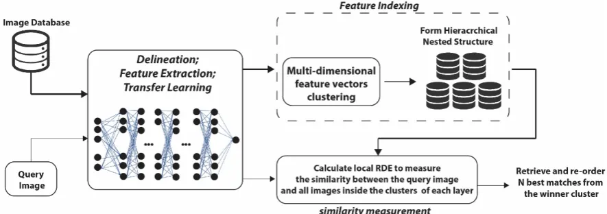
representation, database indexing, and image similarity measurement. Figure1illustrates an overall
J. Imaging2019,5, 33 5 of 21
initial unstructured and structured data sources into analytically prepared data. To achieve a balance between complexity and efficiency, a pre-trained CNN is used to utilize the ability of the model to produce better image representations for the retrieval task. We leverage an existing model trained on
the ImageNet dataset [52], known as residual network (ResNet) [53]. The model is used as a fixed
feature extractor without the last fully connected layer. The trained model provides access to the visual descriptors previously learnt by the CNN after processing millions of images in the ImageNet dataset without requiring a computational expensive training phase.
Journal of Imaging 2019, 5, x FOR PEER REVIEW 5 of 21
a fixed feature extractor without the last fully connected layer. The trained model provides access to the visual descriptors previously learnt by the CNN after processing millions of images in the ImageNet dataset without requiring a computational expensive training phase.
Although the deep learning model is effective in extracting discriminative visual features from images (Section 4.2), it would compute multi-dimensional feature vectors (2048-D in our case) for every image which increases the computational complexity for feature indexing and querying. To address the multi-dimensional complexity caused by the CNN model, a novel nested hierarchical database indexing is proposed to facilitate fast querying. In addition, a recursive calculation based on local density estimation is used to measure the similarity between the given query and all the images from a given image cluster.
Figure 1. Schematic representation of the retrieval model.
3.1. Representation Learning Using Residual Learning Model
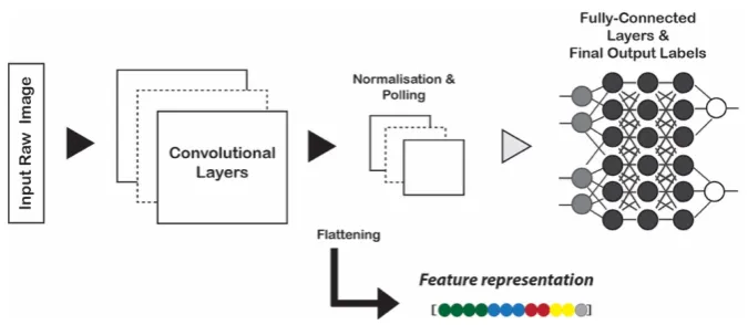
CNNs process images through several layers, mainly in two parts of (a) the convolutional layers and max pooling layers and (b) the fully connected layers which are typically a linear classifier, such as softmax regression classifier (Figure 2). The convolutional layers are used to detect features whereas normalization and pooling layers control overfitting and reduce the number of weights. The last fully-connected layers are used for classification. Recent studies [23,54] indicate that it is feasible to adapt CNN models to extract semantic aware features by the activation of different layers in the networks [52]. Such generic descriptors derived from CNN are effective and powerful.
As mentioned, Neural Networks have the ability to learn and discover a good combination of features, even for complex tasks which would otherwise require a lot of human effort to be manually hand-crafted. In practice, it is common to pre-train a CNN on a very large dataset such as ImageNet dataset with 1.2 million images and 1000 categories, and then use the model either as an initialization for fine-tuning the CNN or use it as a fixed feature extractor, which is also known as Representation Learning (RL). The main reason is that it is relatively rare to have a dataset big enough to train an entire CNN from scratch; additionally, training a CNN model from scratch will take considerable time to train across multiple GPUs on a large-scale dataset such as ImageNet.
Representation learning is the improvement of learning in a new task through the transfer of knowledge from a related task that has already been learned [55]. In such a model, an existing pre-trained model is used as a starting point for a new task, such as classification. The conventional CNNs are treated as end-to-end image classifiers where an image forward propagates through the network and the final probabilities are obtained from the end of the network. However, in the representation learning, instead of allowing the image to forward propagate through the entire network, we can stop the propagation at an arbitrary layer, such as the last fully connected layer, and extract the values from the network at this time, and then use them as feature vectors.
Figure 1.Schematic representation of the retrieval model.
Although the deep learning model is effective in extracting discriminative visual features from
images (Section4.2), it would compute multi-dimensional feature vectors (2048-D in our case) for every
image which increases the computational complexity for feature indexing and querying. To address the multi-dimensional complexity caused by the CNN model, a novel nested hierarchical database indexing is proposed to facilitate fast querying. In addition, a recursive calculation based on local density estimation is used to measure the similarity between the given query and all the images from a given image cluster.
3.1. Representation Learning Using Residual Learning Model
CNNs process images through several layers, mainly in two parts of (a) the convolutional layers and max pooling layers and (b) the fully connected layers which are typically a linear classifier, such as
softmax regression classifier (Figure2). The convolutional layers are used to detect features whereas
normalization and pooling layers control overfitting and reduce the number of weights. The last
fully-connected layers are used for classification. Recent studies [23,54] indicate that it is feasible
to adapt CNN models to extract semantic aware features by the activation of different layers in the
networks [52]. Such generic descriptors derived from CNN are effective and powerful.
As mentioned, Neural Networks have the ability to learn and discover a good combination of features, even for complex tasks which would otherwise require a lot of human effort to be manually hand-crafted. In practice, it is common to pre-train a CNN on a very large dataset such as ImageNet dataset with 1.2 million images and 1000 categories, and then use the model either as an initialization
for fine-tuning the CNN or use it as a fixed feature extractor, which is also known asRepresentation
Learning (RL). The main reason is that it is relatively rare to have a dataset big enough to train an entire CNN from scratch; additionally, training a CNN model from scratch will take considerable time to train across multiple GPUs on a large-scale dataset such as ImageNet.
Representation learning is the improvement of learning in a new task through the transfer of
knowledge from a related task that has already been learned [55]. In such a model, an existing
network and the final probabilities are obtained from the end of the network. However, in the
representation learning, instead of allowing the image to forward propagate through the entire network, we can stop the propagation at an arbitrary layer, such as the last fully connected layer, and extract the values from the network at this time, and then use them as feature vectors.Journal of Imaging 2019, 5, x FOR PEER REVIEW 6 of 21
Figure 2. Representation learning scheme. Deep feature extraction from the pretrained Convolutional Neural Network (CNN) model.
In this study, we utilize the convolutional layers merely as a feature extractor. The aim is to generalize a trained CNN in learning discriminative feature representations for the images in our dataset. The trained model is used to derive feature vectors, more powerful than hand-designed algorithms such as SIFT, GIST, HOG, etc. We exploit the ability of a well-known deep convolutional neural network framework known as residual learning (ResNet) [53,56]. Residual learning frameworks ease the training of deeper networks and are a great candidate to capture the discriminative properties of images as a fixed feature extractor model. Network depth is a key element in neural network architecture; however, deeper networks are more difficult to train, as the accuracy gets saturated and then degrades rapidly. When deeper networks start converging, a degradation problem is exposed which is not caused by overfitting, while adding more layers causes even higher training error. In residual learning models, instead of learning a direct mapping of 𝑥 →
𝑦 with a function 𝐻(𝑥), the residual function is defined using 𝐻(𝑥) = 𝐹(𝑥) + 𝑥; where 𝐹(𝑥) and x
represents residual mapping function and the identity function, respectively. The author's hypothesis is that it is easier to optimize 𝐹(𝑥) than to optimise the original mapping function, 𝐻(𝑥). We refer readers to [53,56] for more details.
The employed ResNet model has been pre-trained on the ImageNet Large Scale Visual Recognition Challenge (ILSVRC) 2012, to classify 1.3 million images to 1000 ImageNet classes [52]. The ResNet consists of convolutional layers, pooling layers, and fully connected layers. The network takes images of size 224 × 224 pixels as input then passes through the network in a forward pass after applying filters to the input image. When treating networks as a fixed feature extractor, we cut off the network at an arbitrary point (normally prior to the last fully-connected layers); thus, all images will be extracted from the activations of convolutional feature maps directly. This would compute a 2048-D feature vector for every image that contains the hidden layer immediately before the classifier. The 2048-D feature vectors will be directly used for computing the similarity between images. The computational complexity and retrieval process may become cumbersome as the dimensionality grows. This requires us to optimize the retrieval process by proposing a hierarchically nested indexing structure and recursive similarity measurements to facilitate faster access and comparison of multi-dimensional feature vectors as described in the following sections.
3.2. Feature Indexing Based on Hierarchical Nested Data Clusters
The success of a CBIR not only depends on image delineation, but feature indexing and similarity measurement matrix also play vital roles to facilitate the execution of queries. In general, feature indexing refers to a database organizing structure to assist fast retrieval process. Whilst it is feasible to retrieve information from datasets which are small in size by measuring the similarity between a query and every image in the dataset, the computational complexity will soon increase significantly on a larger scale image database.
Figure 2.Representation learning scheme. Deep feature extraction from the pretrained Convolutional Neural Network (CNN) model.
In this study, we utilize the convolutional layers merely as a feature extractor. The aim is to generalize a trained CNN in learning discriminative feature representations for the images in our dataset. The trained model is used to derive feature vectors, more powerful than hand-designed algorithms such as SIFT, GIST, HOG, etc. We exploit the ability of a well-known deep convolutional
neural network framework known as residual learning (ResNet) [53,56]. Residual learning frameworks
ease the training of deeper networks and are a great candidate to capture the discriminative properties of images as a fixed feature extractor model. Network depth is a key element in neural network architecture; however, deeper networks are more difficult to train, as the accuracy gets saturated and then degrades rapidly. When deeper networks start converging, a degradation problem is exposed which is not caused by overfitting, while adding more layers causes even higher training error.
In residual learning models, instead of learning a direct mapping of x→y with a functionH(x),
the residual function is defined usingH(x) =F(x) +x; whereF(x)andxrepresents residual mapping function and the identity function, respectively. The author’s hypothesis is that it is easier to optimize
F(x)than to optimise the original mapping function,H(x). We refer readers to [53,56] for more details. The employed ResNet model has been pre-trained on the ImageNet Large Scale Visual Recognition
Challenge (ILSVRC) 2012, to classify 1.3 million images to 1000 ImageNet classes [52]. The ResNet
consists of convolutional layers, pooling layers, and fully connected layers. The network takes images
of size 224×224 pixels as input then passes through the network in a forward pass after applying
filters to the input image. When treating networks as a fixed feature extractor, we cut off the network at an arbitrary point (normally prior to the last fully-connected layers); thus, all images will be extracted from the activations of convolutional feature maps directly. This would compute a 2048-D feature vector for every image that contains the hidden layer immediately before the classifier. The 2048-D feature vectors will be directly used for computing the similarity between images. The computational complexity and retrieval process may become cumbersome as the dimensionality grows. This requires us to optimize the retrieval process by proposing a hierarchically nested indexing structure and recursive similarity measurements to facilitate faster access and comparison of multi-dimensional feature vectors as described in the following sections.
3.2. Feature Indexing Based on Hierarchical Nested Data Clusters
J. Imaging2019,5, 33 7 of 21
is feasible to retrieve information from datasets which are small in size by measuring the similarity between a query and every image in the dataset, the computational complexity will soon increase significantly on a larger scale image database.
In an attempt to address the challenges faced by retrieval information on a large-scale dataset, we present a hierarchically nested structure. The introduced database indexing aims at arranging and structuring the image database into a simple yet effective form of data clusters and hierarchies.
Although forming a hierarchical structure for retrieval optimization has been explored before [57–60],
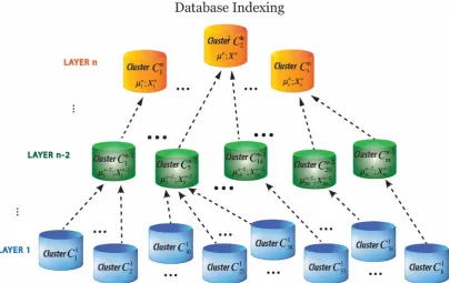
the method presented in this study is quite different. Hierarchically nested data clusters are structured in which data clusters at higher layers represent one or multiple clusters at a lower layer based on
mean values of the cluster centers (Figure3). The first layer clusters are generated based on feature
representations derived from the CNN model. Data clusters are formed by grouping the relevant
data points using a partition-based clustering approach known asK-means clustering [61].Figure3
illustrates how the hierarchical structure of clusters is formed.µandXare abstract values and denote
mean values and scalar products explained in Section3.3.
Journal of Imaging 2019, 5, x FOR PEER REVIEW 7 of 21
In an attempt to address the challenges faced by retrieval information on a large-scale dataset, we present a hierarchically nested structure. The introduced database indexing aims at arranging and structuring the image database into a simple yet effective form of data clusters and hierarchies. Although forming a hierarchical structure for retrieval optimization has been explored before [57– 60], the method presented in this study is quite different. Hierarchically nested data clusters are structured in which data clusters at higher layers represent one or multiple clusters at a lower layer based on mean values of the cluster centers (Figure 3). The first layer clusters are generated based on feature representations derived from the CNN model. Data clusters are formed by grouping the relevant data points using a partition-based clustering approach known as K-means clustering [61].
Figure 3 illustrates how the hierarchical structure of clusters is formed. µ and X are abstract values and denote mean values and scalar products explained in Section 3.3.
Figure 3. Schematic representation of the hierarchical nested indexing structure.
3.3. Fast Searching and Similarity Measure Based on Recursive Data Density Estimation
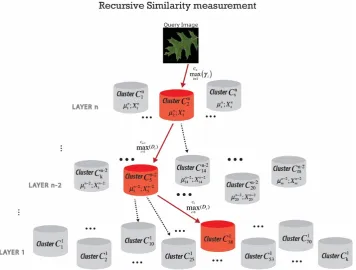
The final step after forming the hierarchically nested data clusters is to find the cluster which contains the most similar images to a query image. We applied recursive density estimation [62,63] to measure a similarity between the query image and all images inside each cluster recursively. The main idea of the recursive density function is to estimate the probability density function by a Cauchy type kernel and to recursively calculate it. The method is also applied for novelty detection in real-time data streams and video analytics [64]. The recursive calculation allows us to discard each data once it has been processed and only store the accumulated information in memory concerning the local mean (per cluster), µ and scalar product X. In order to speed up the retrieval process by an order of magnitude, the searching process is performed from the top of the pyramid in an ordered hierarchy based on “winner takes all” principle with maximum local recursive density estimation at each level (Figure 4).
Figure 3.Schematic representation of the hierarchical nested indexing structure.
3.3. Fast Searching and Similarity Measure Based on Recursive Data Density Estimation
The final step after forming the hierarchically nested data clusters is to find the cluster which
contains the most similar images to a query image. We applied recursive density estimation [62,63] to
measure a similarity between the query image and all images inside each cluster recursively. The main idea of the recursive density function is to estimate the probability density function by a Cauchy type kernel and to recursively calculate it. The method is also applied for novelty detection in real-time
data streams and video analytics [64]. The recursive calculation allows us to discard each data once
it has been processed and only store the accumulated information in memory concerning the local
mean (per cluster),µand scalar product X. In order to speed up the retrieval process by an order of
Figure 4. Schematic representation of searching through hierarchical nested structure and retrieve the most similar images (winner cluster) to the query.
The degree of similarity between the query image to images inside each cluster is measured by the relative local density with regards to the query image, which is defined by a suitable kernel over the distance between the current image sample and all the other images inside the cluster:
𝐷 = 𝐾 𝑑 𝑐 = [1, 𝐶] (1)
where 𝑀 is the number of images associated with cth cluster; 𝑑 denotes the distance between the query image and any other image of the cth cluster; 𝑖 = 1,2, … , 𝑁 ; N is the number of images within
cth cluster.
Different types of distance measures can be used, such as Euclidean or Cosine distance. We used a Cauchy type of kernel to define the local density 𝐷 . It can be proven that Cauchy type kernel asymptotically tends to Gaussian, but can be calculated recursively [63]:
𝐷 = 1
1 + 𝐹 − 𝜇 + 𝑋 − 𝜇 (2)
𝐹 = {𝑓 , ⋯ , 𝑓 } is the feature vector. 𝑖 = 1,2, … , 𝑁 ; Nc is the number of images within cth
cluster.
Both the mean, µi and the scalar product, Xi are updated recursively as follows [63]:
𝜇 =𝑖 − 1
𝑖 𝜇 +
1
𝑖𝐹 ; 𝜇 = 𝐹 (3)
𝑋 =𝑖 − 1
𝑖 𝑋 +
1
𝑖‖𝐹 ‖ ; 𝑋 = ‖𝐹 ‖ (4)
Finally, the cluster with the maximum local density Dc, with respect to the query image, is most likely to contain similar images:
𝐶∗= 𝑎𝑟𝑔𝑚𝑎𝑥 {𝐷 } (5)
Figure 4.Schematic representation of searching through hierarchical nested structure and retrieve the most similar images (winner cluster) to the query.
The degree of similarity between the query image to images inside each cluster is measured by the relative local density with regards to the query image, which is defined by a suitable kernel over the distance between the current image sample and all the other images inside the cluster:
Dic=K Mc
∑
j=1dcij !
c= [1,C] (1)
whereMcis the number of images associated withcthcluster;dcijdenotes the distance between the
query image and any other image of thecthcluster;i=1, 2, . . . ,Nc;Nis the number of images within cthcluster.
Different types of distance measures can be used, such as Euclidean or Cosine distance. We used
a Cauchy type of kernel to define the local densityDc
i. It can be proven that Cauchy type kernel
asymptotically tends to Gaussian, but can be calculated recursively [63]:
Dic= 1
1+kFi−µci k2+Xci− kµci k2 (2)
F = {f1,· · ·,f2048}is the feature vector. i = 1, 2, . . . ,Nc;Nc is the number of images within cthcluster.
Both the mean,µiand the scalar product,Xiare updated recursively as follows [63]:
µi= i−1
i µi−1+
1
iFi;µ1=F1 (3)
Xi = i
−1
i Xi−1+
1
i kFi k 2;X
J. Imaging2019,5, 33 9 of 21
Finally, the cluster with the maximum local densityDc, with respect to the query image, is most
likely to contain similar images:
Ci∗=argmaxCc=1{Dic} (5)
The final step is the similarity measurement between the query image and all the images inside the winning cluster at the lowest layer. The relevance score is defined by distance-based scoring using City Block distance. Images are then ranked accordingly to their obtained scores. A smaller value of City Block distance implies that the corresponding image is more similar to the query image and vice versa. The City Block distance between the query image and images inside the winner cluster is calculated as follows:
dIj,Q=
K
∑
k=1Qk−I
j k
;j=1, . . . ,Nc (6)
whereNcis the number of images of winning cloud;Kis the number of extracted features (K= 2048);
Qdenotes the query image; andIis the image in the winning cluster.
4. Experiments and Results
In this section, we present the experiments conducted to evaluate the key elements of CBIR: accuracy and computational efficiency. The deep learning framework and feature indexing were developed in Python using Keras API and MATLAB, respectively. The experiment was carried out on a desktop PC with Intel Core i7, processing power with 3.4 GHz CPU, 24 GB RAM, and GeForce GT 640 GPU running Ubuntu 16.04. Furthermore, the accuracy of the proposed approach is compared with two hand-crafted feature-based methods, known as BOVW and multiple fused global features (MFF). In addition, the computational efficiency and retrieval execution timing are evaluated against inverted file indexing and non-hierarchical searching.
Integrating multiple features: As mentioned, correct selection and utilizing appropriate features to
represent an image are key elements for having a more accurate retrieval system [65,66]. The common
approach is to combine color and texture properties to generate a robust feature representation [66,67]. In this study, two feature extractor techniques based on color and texture properties known and color
correlogram and GIST are integrated. GIST descriptor [68] is widely used in scene classification to
represent an image by a vector of spectral values which is based on spatial envelope properties, such as ruggedness, expansion, naturalness, and roughness. Color auto-correlogram, on the other hand, is used to preserve the spatial information of colors in an image. It describes the global distribution of local spatial correlations between identical colors [69].
Bag of visual words: In the BOVW method, the SIFT algorithm [18] is applied as a feature
descriptor in addition to Local Linear Constraint (LLC) [70] to project the descriptors into the
visual vocabulary and to reduce the computational complexity. In addition, to preserve the spatial
relationships of the code vector, Spatial Pyramid Matching (SPM) [71] was developed where the entire
image was divided into levels. Each image is divided into spatial sub-regions and histograms of
features are computed from each sub-region. Each level divides the image into 2l×2l−1; wherelis
level. The features are computed locally for each grid and the spatial information is incorporated into histograms. A three-level SPM is comprised of a single histogram in level 0, 4 histograms in level 1, and 16 histograms in level 2. In the end, the histograms from all the sub-regions are concatenated together to generate the final representation of the image. The result is a feature vector of
4.1. Datasets
MalayaKew (MK) Leaf-Dataset: This dataset [72] consists of a collection of leaves from 44 species
class, with 52 images in each class. The data is in the form of digital images, size 256×256 pixels,
collected at the Royal Botanic Garden, Kew, England. The dataset has been used solely for supervised image classification, since the dataset is extremely challenging as some of the classes have very
similar appearances (Figure5) making it extremely difficult to distinguish differences between classes
with a fully unsupervised model, as was presented in this study. Although the MK dataset is not considered a big dataset, we believe the similarity between classes can be a good example to demonstrate how discriminative the features are between the convolutional neural networks and the hand-crafted methods.
Journal of Imaging 2019, 5, x FOR PEER REVIEW 10 of 21
demonstrate how discriminative the features are between the convolutional neural networks and the hand-crafted methods.
Figure 5. Sample images of MalayaKew 44 leaf collection.
The University of California Merced (UCM) Dataset: UCM dataset [73] consists of 21 land cover, large-scale aerial images from the USGS national map urban area imagery. Each class contains 100 images with 256 × 256 pixels; the spatial resolution of each pixel is 30 cm measured in the RGB spectral space. The dataset has been widely utilized for evaluating the performance of high-resolution remote sensing image scene classification [74–76]. The UCM dataset shows very small inter-class diversity among some categories that share a few similar texture patterns or objects, which makes this dataset very challenging. Some sample image scenes from the UCM dataset are shown in Figure 6.
Figure 5.Sample images of MalayaKew 44 leaf collection.
The University of California Merced (UCM) Dataset: UCM dataset [73] consists of 21 land cover, large-scale aerial images from the USGS national map urban area imagery. Each class contains
100 images with 256×256 pixels; the spatial resolution of each pixel is 30 cm measured in the RGB
spectral space. The dataset has been widely utilized for evaluating the performance of high-resolution
remote sensing image scene classification [74–76]. The UCM dataset shows very small inter-class
diversity among some categories that share a few similar texture patterns or objects, which makes this
J. Imaging2019,5, 33 11 of 21
Journal of Imaging 2019, 5, x FOR PEER REVIEW 11 of 21
Figure 6. Sample images of the University of California Merced (UCM) dataset.
4.2. Performance and Accuracy
Throughout this work, we use two evaluation metrics widely used to assess CBIR performance, known as mean Average Precision (mAP) and the precision at rank N (P@N). Average Precision (AP) is one of the most frequent methods used to evaluate the retrieval quality of a single query’s retrieval results. AP takes consideration of both Precision (Pr) and Recall (Re). Precision is the fraction of retrieved images that are relevant, whereas Recall is the fraction of relevant images that are retrieved.
AP averages the precision values from the rank positions where relevant images are retrieved. The mean average precision (mAP) is widely used to summaries the retrieval quality, which averages the
AP over all queries. The definition of the above metrics follows below [4]:
𝐴𝑃 =∑ 𝑃(𝑘) × 𝑟𝑒𝑙(𝑘)
𝑅 (7)
where P(k) denotes the precision of top k retrieval results; rel(k) is a binary indicator function equaling 1 if the kth retrieved results are relevant to the current query image and 0 otherwise; and R and n denote the number of relevant results for the current query image and the total number of retrieved results, respectively. Also, the precision at particular rank-N accuracy is another evaluation metric to evaluate CBIR performance. P@N score refers to the average number of same retrieved images, within the top-N ranked images. It should be noted that although mAP and P@N are widely used as evaluation metrics in CBIR, defining a suitable metric to measure the quality of results for an arbitrary query image is not a trivial process. In CBIR, it is hard to define the ground-truth since different users might have a different measure of similarity. If the degree of similarity of some of the images is very low, ignoring or not displaying those images is not critical and does not impact the overall performance of the system. Labelling images as non-relevant is not always satisfactory to the users. Any CBIR should have a certain tolerance for false positives, which often provides useful information.
In this study, to form a hierarchically nested pyramid, at the lower layer, images were grouped into a fixed number of clusters, while at the second layer, the means of the clusters at the first layer were further grouped into smaller numbers of clusters. Since the number of images in both datasets
Figure 6.Sample images of the University of California Merced (UCM) dataset.
4.2. Performance and Accuracy
Throughout this work, we use two evaluation metrics widely used to assess CBIR performance,
known as mean Average Precision (mAP) and the precision at rankN(P@N). Average Precision (AP) is
one of the most frequent methods used to evaluate the retrieval quality of a single query’s retrieval
results. APtakes consideration of both Precision (Pr) and Recall (Re). Precision is the fraction of
retrieved images that are relevant, whereas Recall is the fraction of relevant images that are retrieved.
APaverages the precision values from the rank positions where relevant images are retrieved. The mean
average precision (mAP) is widely used to summaries the retrieval quality, which averages theAPover
all queries. The definition of the above metrics follows below [4]:
AP= ∑
n
k=1P(k)×rel(k)
R (7)
whereP(k)denotes the precision of topkretrieval results;rel(k)is a binary indicator function equaling 1
if thekthretrieved results are relevant to the current query image and 0 otherwise; andRandndenote
the number of relevant results for the current query image and the total number of retrieved results,
respectively. Also, the precision at particular rank-Naccuracy is another evaluation metric to evaluate
CBIR performance. P@Nscore refers to the average number of same retrieved images, within the
top-Nranked images. It should be noted that althoughmAPandP@Nare widely used as evaluation
metrics in CBIR, defining a suitable metric to measure the quality of results for an arbitrary query image is not a trivial process. In CBIR, it is hard to define the ground-truth since different users might have a different measure of similarity. If the degree of similarity of some of the images is very low, ignoring or not displaying those images is not critical and does not impact the overall performance of the system. Labelling images as non-relevant is not always satisfactory to the users. Any CBIR should have a certain tolerance for false positives, which often provides useful information.
J. Imaging2019,5, 33 12 of 21
in the region of few thousands, two-layer hierarchies are enough to achieve real-time image querying. In MK and UCM datasets, based on our experience, the number of clusters at the first layer was set to 44 and 21 clusters (number of categories) and 10 and 4 clusters at the top layer, respectively.
The retrieval process begins by calculating the local recursive density estimation between the query image and all the clusters at the top layer and selecting the winning cluster with maximum local Recursive Density Estimation (RDE). The search continues at the lower layers, but only with the clusters which associated to the winning cluster at the top layer. Finally, images in the winning cluster at the lowest stage are ranked based on calculating the eigenvector distance to the query image.
4.2.1. Retrieval Performance on MalayaKew Leaf-Dataset
The results of the convolutional neural network as a feature extractor (RL-CNN) are shown in
Figure7and Table1. The precision accuracy at rank-20 is compared in Figure7based on 20 queries.
The queries were selected to tackle every range of visual appearances with a unique shape, such as
qoxyodon, or similar appearances, likeq-aff-cerrisandqlaurifolia.
is in the region of few thousands, two-layer hierarchies are enough to achieve real-time image querying. In MK and UCM datasets, based on our experience, the number of clusters at the first layer was set to 44 and 21 clusters (number of categories) and 10 and 4 clusters at the top layer, respectively. The retrieval process begins by calculating the local recursive density estimation between the query image and all the clusters at the top layer and selecting the winning cluster with maximum local Recursive Density Estimation (RDE). The search continues at the lower layers, but only with the clusters which associated to the winning cluster at the top layer. Finally, images in the winning cluster at the lowest stage are ranked based on calculating the eigenvector distance to the query image.
4.2.1. Retrieval Performance on MalayaKew Leaf-Dataset
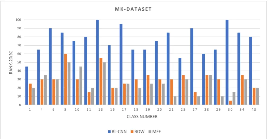
The results of the convolutional neural network as a feature extractor (RL-CNN) are shown in Figure 7 and Table 1. The precision accuracy at rank-20 is compared in Figure 7 based on 20 queries. The queries were selected to tackle every range of visual appearances with a unique shape, such as
qoxyodon, or similar appearances, like q-aff-cerris and qlaurifolia.
Several observations can be achieved from the precision results. The RL-CNN method outperformed the two state-of-the-art techniques by a large margin. The proposed method not only performed well on classes with unique visual appearances, such as qlobata or qpetraea, but it also distinguished categories with similar appearances, such as quercus and q-x-kewensis. In RL-CNN method, q-x-mannifera, qboissieri, qellipsoidalis, qmacransmera, and qpetraea obtained maximum accuracy with over 90%, whereas qlaurifolia and q-aff-cerris had the lowest value of 55% and 45%, respectively. The qlaurifolia class achieved 55% accuracy, whereas 9 out of 20 images belong to
qcanariensis, qrhysophylla, and qtrotana categories (Figure 8A). The accuracy dropped to 35% and 30% in BOVW and MFF, accordingly. The q-aff-cerris class obtained the lowest accuracy in RL-CNN with 45% accuracy rate, whereas 11 out of 20 images belong to qrobur category, which is visually almost identical to the query image.
Figure 7. The retrieval Rank-20 accuracy between the Convolutional Neural Network (CNN) as a feature extractor, bag of visual words, and multiple feature fusion (color and texture).
On the other hand, the BOVW and MFF performed poorly in identifying small differences between leaf varieties in MK dataset. Both methods retrieved images with the visual similarity to queries; however, they failed to distinguish small visual differences among classes. As illustrated in Figure 7, BOVW performed better than MFF in most cases, except classes q_rubur_f_purpubascens, qagriefolia, qagrifolia, and qpetraea. (The results for each class are presented in the Supplementary Materials).
0 10 20 30 40 50 60 70 80 90 100
1 4 6 8 1 0 1 1 1 3 1 6 1 7 1 8 1 9 2 0 2 1 2 5 2 7 2 8 2 9 3 0 3 4 4 3
RANK-20(%)
CLASS NUMBER M K - D A T A S E T
RL-CNN BOW MFF
Figure 7. The retrieval Rank-20 accuracy between the Convolutional Neural Network (CNN) as a feature extractor, bag of visual words, and multiple feature fusion (color and texture).
Table 1.The retrieval accuracymAPof convolutional neural network as a feature extractor (RL-CNN), bag of visual words (BOVW), and multiple fused global features (MFF) on Malaya–Kew (MK) and University of California Merced (UCM) datasets.
Dataset Method mAP(%)
MalayaKew
FE-CNN 88.1% BOVW 66.2%
MFF 52.6%
UCM
FE-CNN 90.5% BOVW 86.2%
MFF 69.8%
Several observations can be achieved from the precision results. The RL-CNN method
outperformed the two state-of-the-art techniques by a large margin. The proposed method not
only performed well on classes with unique visual appearances, such asqlobataorqpetraea, but it
J. Imaging2019,5, 33 13 of 21
method,q-x-mannifera,qboissieri,qellipsoidalis,qmacransmera, andqpetraeaobtained maximum accuracy
with over 90%, whereasqlaurifoliaandq-aff-cerrishad the lowest value of 55% and 45%, respectively.
The qlaurifolia class achieved 55% accuracy, whereas 9 out of 20 images belong to qcanariensis,
qrhysophylla, andqtrotanacategories (Figure8A). The accuracy dropped to 35% and 30% in BOVW and
MFF, accordingly. Theq-aff-cerrisclass obtained the lowest accuracy in RL-CNN with 45% accuracy
rate, whereas 11 out of 20 images belong toqroburcategory, which is visually almost identical to the
query image.Journal of Imaging 2019, 5, x FOR PEER REVIEW 13 of 21
Figure 8. Qualitative evaluation of the proposed image retrieval on the two lowest performance of classes in Malaya–Kew Leaf-Dataset (A) Retrieval result from qlaurifolia class (B) retrieval result from q-aff-cerris class. The first image is the query and the following images are the images most similar to the query image. The retrieved images wrongly categorized are highlighted in red.
Table 1 summarizes the mAP evaluation of the Malaya–Kew leaf dataset. The results are obtained from 20 queries in which the retrieval system can be tested and evaluated. The best accuracy score is 88.1%, achieved by RL-CNN, followed by BOVW and MFF with 66.2% and 52.6%, respectively.
Table 1. The retrieval accuracy mAP of convolutional neural network as a feature extractor (RL-CNN), bag of visual words (BOVW), and multiple fused global features (MFF) on Malaya–Kew (MK) and University of California Merced (UCM) datasets.
Dataset Method mAP (%)
MalayaKew
FE-CNN 88.1% BOVW 66.2% MFF 52.6%
UCM
FE-CNN 90.5% BOVW 86.2% MFF 69.8%
4.2.2. Retrieval Performance on UCM Dataset
The precision performances at P@40 for the UCM dataset are shown in Figure 9. The results show that RL-CNN method outperformed both the BOW and MFF by achieving better accuracy in all categories except baseball diamond category. In RL-CNN, high accuracy results obtained in agricultural, beach, forest, harbor, chaparral, and airplane (Figure 10) categories. On the other hand, in the baseball-diamond, dense residential (Figure 11), and freeway (Figure 12), RL-CNN achieved the lowest accuracy with 41%, 35%, and 50%, respectively (Figure 9).
Figure 8.Qualitative evaluation of the proposed image retrieval on the two lowest performance of classes in Malaya–Kew Leaf-Dataset (A) Retrieval result from qlaurifolia class (B) retrieval result from q-aff-cerris class. The first image is the query and the following images are the images most similar to the query image. The retrieved images wrongly categorized are highlighted in red.
On the other hand, the BOVW and MFF performed poorly in identifying small differences between leaf varieties in MK dataset. Both methods retrieved images with the visual similarity to queries;
however, they failed to distinguish small visual differences among classes. As illustrated in Figure7,
BOVW performed better than MFF in most cases, except classesq_rubur_f_purpubascens, qagriefolia,
qagrifolia, andqpetraea. (The results for each class are presented in the Supplementary Materials).
Table1summarizes themAPevaluation of the Malaya–Kew leaf dataset. The results are obtained
from 20 queries in which the retrieval system can be tested and evaluated. The best accuracy score is 88.1%, achieved by RL-CNN, followed by BOVW and MFF with 66.2% and 52.6%, respectively.
4.2.2. Retrieval Performance on UCM Dataset
The precision performances atP@40 for the UCM dataset are shown in Figure9. The results
show that RL-CNN method outperformed both the BOW and MFF by achieving better accuracy
in all categories except baseball diamondcategory. In RL-CNN, high accuracy results obtained in
agricultural,beach,forest,harbor,chaparral, andairplane(Figure10) categories. On the other hand, in the
baseball-diamond,dense residential(Figure11), andfreeway(Figure12), RL-CNN achieved the lowest
accuracy with 41%, 35%, and 50%, respectively (Figure9).
Figure11 shows the retrieval results of the dense buildingclass on a randomly given query.
The class achieved 35% accuracy, whereas 14 out of 40 images belong to the same class as the query
image. However, the rest of the images are still visually similar to the query retrieved frommedium
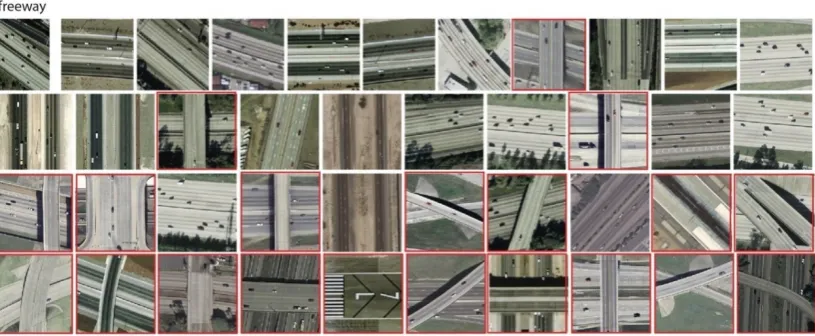
residentialandmobile home parkclasses. Thefreewayclass with 50% accuracy has a similar performance,
whereas half of the retrieved images belong torunwayandoverpassclasses, which are still visually very
J. Imaging2019,5, 33 14 of 21
Journal of Imaging 2019, 5, x FOR PEER REVIEW 14 of 21
Figure 9. The retrieval Rank-40 accuracy between feature extractor using convolutional neural network, bag of visual words, and multiple feature fusion (color and texture).
Figure 11 shows the retrieval results of the dense building class on a randomly given query. The class achieved 35% accuracy, whereas 14 out of 40 images belong to the same class as the query image. However, the rest of the images are still visually similar to the query retrieved from medium residential and mobile home park classes. The freeway class with 50% accuracy has a similar performance, whereas half of the retrieved images belong to runway and overpass classes, which are still visually very similar to the freeway class (Figure 12).
Figure 10. Retrieval results of airplane category using convolutional neural network as a feature extractor (RL-CNN). The methods obtained 100% retrieval accuracy.
0 10 20 30 40 50 60 70 80 90 100
Rank-40
UCM-Dataset
RL-CNN BOW MFF
Figure 9.The retrieval Rank-40 accuracy between feature extractor using convolutional neural network, bag of visual words, and multiple feature fusion (color and texture).
Figure 9. The retrieval Rank-40 accuracy between feature extractor using convolutional neural network, bag of visual words, and multiple feature fusion (color and texture).
Figure 11 shows the retrieval results of the dense building class on a randomly given query. The class achieved 35% accuracy, whereas 14 out of 40 images belong to the same class as the query image. However, the rest of the images are still visually similar to the query retrieved from medium residential and mobile home park classes. The freeway class with 50% accuracy has a similar performance, whereas half of the retrieved images belong to runway and overpass classes, which are still visually very similar to the freeway class (Figure 12).
Figure 10. Retrieval results of airplane category using convolutional neural network as a feature extractor (RL-CNN). The methods obtained 100% retrieval accuracy.
0 10 20 30 40 50 60 70 80 90 100
Rank-40
UCM-Dataset
RL-CNN BOW MFF
Figure 10. Retrieval results of airplane category using convolutional neural network as a feature extractor (RL-CNN). The methods obtained 100% retrieval accuracy.
Journal of Imaging 2019, 5, x FOR PEER REVIEW 15 of 21
Figure 11. Retrieval results of dense-building category using convolutional neural network as a feature extractor (RL-CNN). The green rectangles indicate correct retrieval results.
Figure 12. Retrieval results of freeway category using convolutional neural network as a feature extractor (RL-CNN). The red rectangles indicate incorrect retrieval results.
The retrieval mAP of different models on the UCM image dataset are listed in Table 1. As shown in the table, the RL-CNN outperformed both the state-of-the-art techniques. The mAP measure in RL-CNN is 90.1%, whereas the BOW and MFF achieved 86.2% and 69.8%, respectively.
4.3. Retrieval Time Per Query
Commercial CBIR applications are often assessed for requirements in computational capacity and memory efficiency. As mentioned earlier, the proposed hierarchically nested structure is beneficial for the retrieval performance in terms of search time and memory size required to store the indexed images. In this section, we provide more details on the retrieval time per query between the proposed method, the inverted index file method, and the non-hierarchical searching with a single layer. The non-hierarchical searching technique processes each image by scanning all image patches and computing similarity values for every individual image, unlike the nested hierarchical indexing described in Section 3.2.
Figure 13 shows the execution time of CNN-hierarchically nested structure, CNN sequential searching, BOVW-inverted indexing technique, and BOVW-non-hierarchical retrieval method. The non-hierarchical method processes each image by scanning all images and computing similarity values between query images and all images. In contrast, the hierarchically nested indexing avoids comparing the query image with every image in the dataset by grouping similar images together and measures the similarity based on recursive density estimation. The inverted index technique also
J. Imaging2019,5, 33 15 of 21
Journal of Imaging 2019, 5, x FOR PEER REVIEW 15 of 21
Figure 11. Retrieval results of dense-building category using convolutional neural network as a feature extractor (RL-CNN). The green rectangles indicate correct retrieval results.
Figure 12. Retrieval results of freeway category using convolutional neural network as a feature extractor (RL-CNN). The red rectangles indicate incorrect retrieval results.
The retrieval mAP of different models on the UCM image dataset are listed in Table 1. As shown in the table, the RL-CNN outperformed both the state-of-the-art techniques. The mAP measure in RL-CNN is 90.1%, whereas the BOW and MFF achieved 86.2% and 69.8%, respectively.
4.3. Retrieval Time Per Query
Commercial CBIR applications are often assessed for requirements in computational capacity and memory efficiency. As mentioned earlier, the proposed hierarchically nested structure is beneficial for the retrieval performance in terms of search time and memory size required to store the indexed images. In this section, we provide more details on the retrieval time per query between the proposed method, the inverted index file method, and the non-hierarchical searching with a single layer. The non-hierarchical searching technique processes each image by scanning all image patches and computing similarity values for every individual image, unlike the nested hierarchical indexing described in Section 3.2.
Figure 13 shows the execution time of CNN-hierarchically nested structure, CNN sequential searching, BOVW-inverted indexing technique, and BOVW-non-hierarchical retrieval method. The non-hierarchical method processes each image by scanning all images and computing similarity values between query images and all images. In contrast, the hierarchically nested indexing avoids comparing the query image with every image in the dataset by grouping similar images together and measures the similarity based on recursive density estimation. The inverted index technique also
Figure 12. Retrieval results of freeway category using convolutional neural network as a feature extractor (RL-CNN). The red rectangles indicate incorrect retrieval results.
The retrievalmAPof different models on the UCM image dataset are listed in Table1. As shown
in the table, the RL-CNN outperformed both the state-of-the-art techniques. ThemAPmeasure in
RL-CNN is 90.1%, whereas the BOW and MFF achieved 86.2% and 69.8%, respectively.
4.3. Retrieval Time Per Query
Commercial CBIR applications are often assessed for requirements in computational capacity and memory efficiency. As mentioned earlier, the proposed hierarchically nested structure is beneficial for the retrieval performance in terms of search time and memory size required to store the indexed images. In this section, we provide more details on the retrieval time per query between the proposed method, the inverted index file method, and the non-hierarchical searching with a single layer. The non-hierarchical searching technique processes each image by scanning all image patches and computing similarity values for every individual image, unlike the nested hierarchical indexing described in Section3.2.
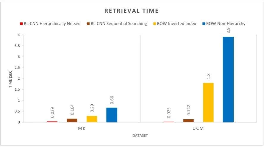
Figure13shows the execution time of CNN-hierarchically nested structure, CNN sequential
searching, BOVW-inverted indexing technique, and BOVW-non-hierarchical retrieval method. The non-hierarchical method processes each image by scanning all images and computing similarity values between query images and all images. In contrast, the hierarchically nested indexing avoids comparing the query image with every image in the dataset by grouping similar images together and measures the similarity based on recursive density estimation. The inverted index technique also avoids performing a linear search over all images in the dataset, helping us to speed up the querying process. In the inverted index method, we query our inverted index to find images that contain the same visual word as the query image. Then, we only compare images in the dataset that contain a significant number of visual words as the query.
As illustrated in Figure 13, the proposed hierarchical indexing method achieved the fastest
retrieval performance. The average retrieval time of RL-CNN with hierarchical indexing scheme on the MK and UCM image datasets are 0.039 and 0.025 seconds, respectively. RL-CNN with sequential
searching came second with 0.164 and 0.142 seconds, respectively. Nevertheless, this is anO(N)linear
operation; thus, the execution time increases considerably in the sequential searching if the number of images increases to hundreds of thousands or millions. BOVW with inverted index and BOVW without indexing had the slowest retrieval time, with 0.29 and 1.8 seconds and 0.66 and 3.9 seconds in MK and UCM datasets, respectively. Moreover, the RL-CNN with sequential searching showed faster performance compared to the BOW with a similar structure. This can be justified since the RL-CNN