Assessment of empirical algorithms for bathymetry extraction using Sentinel-2 data

Full Terms & Conditions of access and use can be found at

http://www.tandfonline.com/action/journalInformation?journalCode=tres20

International Journal of Remote Sensing

ISSN: 0143-1161 (Print) 1366-5901 (Online) Journal homepage: http://www.tandfonline.com/loi/tres20

Assessment of empirical algorithms for

bathymetry extraction using Sentinel-2 data

Gema Casal, Xavier Monteys, John Hedley, Paul Harris, Conor Cahalane &

Tim McCarthy

To cite this article: Gema Casal, Xavier Monteys, John Hedley, Paul Harris, Conor Cahalane & Tim McCarthy (2018): Assessment of empirical algorithms for bathymetry extraction using Sentinel-2 data, International Journal of Remote Sensing

To link to this article: https://doi.org/10.1080/01431161.2018.1533660

Published online: 22 Oct 2018.

Submit your article to this journal

Assessment of empirical algorithms for bathymetry

extraction using Sentinel-2 data

Gema Casala_{, Xavier Monteys}b_{, John Hedley}c_{, Paul Harris} d_{, Conor Cahalane}e and Tim McCarthya

a_{National Centre for Geocomputation, Maynooth University, Maynooth, Co. Kildare, Irelan;}b_Geological Survey Ireland, Dublin, Ireland;c_{Numerical Optics Ltd, Dublin City, Devon, UK;}d_{Sustainable Soil and} Grassland Systems, Rothamsted Research, Devon, UK;e_{School of Surveying and Construction} Management, Dublin Institute of Technology, Dublin, Ireland

ABSTRACT

Bathymetry estimated from optical satellite imagery has been increasingly implemented as an alternative to traditional bathy-metric survey techniques. The availability of new sensors such as Sentinel-2 with improved spatial and temporal resolution, in com-parison with previous optical sensors, offers innovative capabilities for bathymetry derivation. This study presents an assessment of thefit between satellite data and the underlying models in the most widely used empirical algorithms: the linear band model and the log-transformed band ratio model using Sentinel-2A data. Both models were tested in two study areas of the Irish coast with different morphological and environmental conditions. Results showed that the linear band modelfitted better than the log-transformed band ratio model providing coefficient of deter-mination values, R2, between 0.83 and 0.88 (0 m–10 m) for thefive images considered in the study. The closestfit was found in the depth range 2 m–6 m. Atmospheric correction, bottom type infl u-ence, and water column conditions proved to be key factors in the bathymetric derivation using these satellite datasets.

ARTICLE HISTORY

Received 1 May 2018 Accepted 11 August 2018

KEYWORDS

Bathymetry; empirical algorithm; atmospheric correction; coastal applications

1. Introduction

Timely and accurate environmental information such as bathymetry is necessary to support effective resource policy and management for coastal areas as well as to assure human security and welfare. Bathymetry derived from optical satellite data has been increasingly implemented as an alternative to traditional bathymetric survey techniques. Nevertheless, when it comes to the successful application of these methods in coastal environments, several challenges need to be considered.

The complex composition of the water column in coastal areas can impede the bathymetry extraction, both through reduction in the clarity of the water, and through confounding factor of spatial variability. Atmospheric correction is also considered a critical step in the analyses of satellite data related to aquatic environments, including the ones related to bathymetric extraction (e.g. Bramante, Raju, and Sin 2013; Hedley

CONTACTGema Casal [email protected] https://doi.org/10.1080/01431161.2018.1533660

et al. 2012; Eugenio et al. 2017). At satellite altitude, about 90% of sensor-measured signal corresponds to atmospheric and surface effects (Gordon and Morel1983). Hence, it is crucial to have an accurate atmospheric correction as 0.5% error in atmospheric correction or calibration can involve an approximate error of 5.0% in the derived water-leaving radiance (IOCCG2010).

Due to their complexity, coastal waters have more demanding requirements for the instrument spectral resolution and sensitivity, atmospheric correction accuracy and water constituent retrieval algorithms. This issue becomes especially important in multi-temporal studies where the analysis of the images needs to be done on a comparable basis; the influence of the atmosphere can be variable between images compromising the results. Adjacency effects due to the surrounding lands also complicate the atmospheric correc-tion procedures, especially in areas surrounded by elevated terrain. Another aspect to consider in aquatic applications is the sun glint. The sunglint effect consists in the specular reflection of light from the water surface and can be considered one of the greatest confounding factors that limit the quality and accuracy of remotely sensed data (Kay, Hedley, and Lavender2009). Sunglint is a function of the sea surface state, sun position, and viewing angle as it occurs when the water surface orientation is such that the sun is directly reflected towards the sensor (Kay, Hedley, and Lavender2009).

Despite these constraints, satellite-derived bathymetry is a cost-effective alternative methodology that, dependent on imagery spatial resolution, provides high-resolution mapping over a wide area rapidly and efficiently. In recent years many studies have been published using airborne (e.g. Chust et al. 2010; Vathmäe and Kutser 2016) and spaceborne sensors (e.g. Lyons, Phinn, and Roelfsema 2011; Kabiri 2017) to derive the bottom depth. Most of these studies have used empirical methods assuming that light is attenuated exponentially with depth and this attenuation is wavelength dependent. Even applied in less extent, in part for their higher data and computing requirements, physics-based methods are also used to derive bathymetry from airborne and space-borne sensors (Brando et al. 2009; Dekker et al. 2011). The physics-based method assumes that water optical properties can vary from pixel to pixel across the image and coefficients, along with other retrievable parameters (water quality, benthic com-munity endmember composition, and water depth), are deduced for every pixel by the best modelfit within the constraints (Hamylton, Hedley, and Beaman2015).

The technical capabilities offered by the Sentinel-2 satellites provide unique charac-teristics for mapping these shallow coastal areas. Sentinel-2 satellites carry a single Multi-Spectral Instrument (MSI) with 13 spectral channels ranging from the Visible and the Near Infrared (VNIR) to the Shortwave Infrared (SWIR) with a spatial resolution of 10 m, 20 m and 60 m. The Sentinel-2 mission is based on a constellation of two identical satellites in the same orbit, phased at 180º to each other. Both satellites, Sentinel-2A and Sentinel-2B provide an optimal coverage of Earth’s land surfaces, large islands as well as inland and coastal waters with a joint revisit time of 5 days. Preliminary results have already suggested the potential of Sentinel-2 in inland waters (Toming et al. 2016; Liu et al.2017), coral reefs (Hedley et al.2012,2018) and diverse coastal applications (e.g. Salama, Radwan, and van der Velde 2012; Gernez et al. 2015). However, bathymetry focussed applications are still scarce (e.g. Chybiki2017; Kabiri2017; Traganos et al.2018) especially in optically complex coastal waters, such as the Irish coast.

Therefore, the main aim of this study is to assess the extent to which two of the most widely used empirical algorithms, the linear band model (Lyzenga1978,1985; Lyzenga, Malinas, and Tanis2006) and the log-transformed band ratio model (Stumpf, Holderied, and Sinclair 2003), provide an accurate model for bathymetry using Sentinel-2 data. These models will be assessed in two study areas of the Irish coast. A complementary comparison of several atmospheric processors will be done through the assessment of the relationship between water depth and reflectance at certain bands.

2. Material and methods

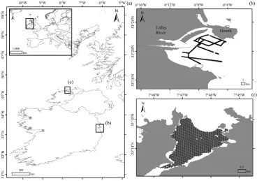
2.1. Study areas

2005). The spring bloom occurs between April and May with a mean chlorophyll concentration ranging between 2.2 µg L−1 and 5.5 µg L−1 (O’Boyle and Silke 2010). High biomass phytoplankton blooms are also frequent in this area.

Mulroy Bay (MB) is the most convoluted of the marine inlets in north-west Ireland being approximately 12 km long in a north-south direction. It has been described as a fully marinefiordic inlet, a glacially derived embayment in low-lying land situated on the northern coast of County Donegal (Figure 1). Mulroy Bay can be divided into four main areas: The Outer Bay, Northwater, Broadwater, and the Channel (also known by The Narrows). Only the‘The Outer Bay’will be considered in this study. This area comprises the most external part of the bay in communication with the open sea waters. Maximum depths within the bay relative to chart datum are 47 m in Northwater and 40 m in Broadwater, being shallower nearer ‘The Narrows’ and deeper in the basin. Approximately, 62% of the total surface area has a depth of 0 m–10 m, while 28% is between 10 m and 20 m and 10% is between 20 m and 47 m (Moreno-Navas, Telfer, and Ross2011). The tidal range varies on average from about 3.70 m (neap to spring) at the mouth of the Outer Bay to about 1.40 m in Broadwater (Moreno-Navas, Telfer, and Ross

2011). The area represents a wind-driven scenario as it suffers frequent strong winds, mainly from the south and south-west. Bar rocks and high rocks, exposed at low tide, are navigational hazards in the centre of the bay. Studies carried out in Mulroy Bay reported total chlorophyll concentrations to be low (about 2.0 µg L−1) for most of the year with only occasional peaks in February and March (>5.0 µg L−1) (Telfor and Robinson2003). Mulroy Bay is one of the most intensively farmed aquatic areas in Ireland affecting its

water quality conditions. However, this effect is more pronounced at the Broadwater and the Northwater (Telfor and Robinson2003), areas not considered in this study.

2.2. In situ data

In Dublin Bay, bathymetry data were collected on board the research vessel Lir as part of the INFOMAR Programme. Several multibeam survey lines and transects were acquired on the 25 July 2017 and processed using the hydrographic CARIS HIPS

™

suite (Figure 1). Vertical tidal corrections were applied and reduced to Lowest Astronomical Tide (LAT). Depth data meets the International Hydrographic Organization (IHO) order 1 standards. Between 0 m and 10 m water depth, position uncertainty and the depth error uncertainty are less than 0.50 m and 0.10 m, respectively. The horizontal spatial resolution of the ungridded data is circa 0.20 cm × 0.20 cm. In the case of Mulroy Bay bathymetry data were acquired on the 11 September 2005 and 12 September 2005 using airborne LiDAR (Figure 1). Vertical tidal corrections were applied and reduced to LAT. Position uncertainty was less than 1 m, and the vertical error uncertainty is approximately 0.5 m. The horizontal spatial resolution of the ungridded data is circa 4 m × 4 m. In both cases, the data were gridded to 5 m × 5 m using an Inverse Distance Weighted algorithm (IDW) and subsequently randomly reduced to approximately 2,000 data points to optimise computing procedures. Only water depths between 0 m and 10 m were considered for the subsequent analysis.

2.3. Satellite data and pre-processing

The cloud coverage and water column conditions (e.g. presence of suspension material and swell), hampered the number of suitable images available for Irish coast in most of the months. A total of five Sentinel-2A images, two images for Dublin Bay and three images for Mulroy Bay, were considered (Table 1). Sentinel products were downloaded from the Copernicus Scientific Data Hub website as level-1C, Top Of Atmosphere (TOA) reflectance in 100 km × 100 km tiles formats and a Universal Transverse Mercator (UTM)/ World Geodetic System 1984 (WGS84) projection. All the images were affected by sun glint to greater or less extent.

Only the 10 m spatial resolution bands B2 (497 nm), B3(560 nm), B4(665 nm) were

considered. A preliminary analysis including band B1(444 nm) was carried out but due to its

lower spatial resolution (60 m), its higher Signal to Noise Ratio (SNR) (Pahlevan et al.2017a) and its high collinearity with B2, B1was ultimately ruled out for further analysis.

Table 1.Details of the Sentinel-2 (S2) images included in the study. Acquisition time is provided in Coordinated Universal Time (UTC). Tide height (m) information was provided by the Irish National Tide Gauge Network at the stations. Wind speed (m s−1) was provided by the Dublin Bay Buoy and the Foyle Buoy for Dublin Bay and Mulroy Bay, respectively. Both buoys are part of the meteor-ological and oceanographic (MetOcean) sensors network.

Study area S2-granule Code Date Acquisition time (UTC) Tide height (m) Wind (m s−1₎

Dublin bay T29UPV DB1 17 June 2017 11:33 1.29 2.57

DB2 17 July 2017 11:33 1.25 6.17

Mulroy bay T29UNB MB1 4 May 2017 11:54 2.51 6.69

MB2 20 June 2017 11:43 1.99 4.63

Before the application of the empirical bathymetric models, all the images were resized to the defined study areas (Figure 2) and atmospherically corrected. Currently, several open source atmospheric correction algorithms are available for Sentinel-2. In this study Atmospheric correction for OLI‘lite’(ACOLITE), the Sentinel-2 data Correction (Sen2Cor version 2.4), the Image correction for atmospheric effects (iCOR) and the Case 2 Regional CoastColour processor (C2RCC) were tested. All of them use the image-based

approach; that means that all input data required for the atmospheric correction are derived from the image itself or provided through pre-calculated look up tables. Sen2Cor, C2RCC and iCOR are available through the European Space Agency (ESA)’s Sentinel toolbox in the Sentinel Application Platform (SNAP).

ACOLITE is an automatic method for atmospheric correction that can be applied over extremely turbid waters using SWIR bands (Vanhellemont and Ruddick 2015). Atmospheric correction of satellite imagery over turbid waters requires separation of aerosol and marine contributions from the TOA signal observed by the satellite. It assumes that due to extremely high pure water absorption in the SWIR bands the signal remaining in these bands after Rayleigh correction is caused by aerosol scattering. The SWIR bands are used both for water pixel detection and aerosol correction. ACOLITE was specifically developed for marine and inland waters (Vanhellemont and Ruddick 2016). User can define the output in remote sensing reflectances.

Sen2Cor is a semi-empirical algorithm based on the Atmospheric and Topographic Correction (ATCOR) that was initially developed for its application to terrestrial environ-ments. The processing starts with the Cloud Detection and Scene Classification followed by the retrieval of the Aerosol Optical Thickness (AOT) and the Water Vapour (WV) content from the level-1C image. The final step is the TOA to Bottom Of Atmosphere (BOA) conversion (Louis et al. 2016). The implemented algorithm requires Dense Dark Vegetation (DDV) pixels in the image for AOT retrieval (Louis et al.2016). The generated output contains BOA reflectance.

iCOR, previously known as Operational Atmospheric Correction for Land and Water (OPERA) (Sterckx et al.2015a), allows atmospheric correction over land, inland, and water coastal waters with a treatment of water surface reflectance. The workflow of iCOR can be summarized in the following steps: 1) land and water pixels identification 2) land pixels used to derive AOT (Guanter 2007) 3) adjacency correction performed using SIMilarity Environment Correction (SIMEC) (Sterckx et al.2015b) and 4) the radiative transfer equation solved. iCOR uses MODerate resolution atmospheric TRANsmission (MODTRAN) 5 Look up Tables (LUT) to perform atmospheric correction and needs information about solar and viewing angles. The generated output contains BOA reflectance.

C2RCC was firstly introduced in the 1990’s as a processor for the Medium Resolution Imaging Spectrometer (MERIS) sensor devoted to inland waters (MERIS Lakes Processor) and subsequently, an improved version was used in the MERIS 3rdReprocessing which is the current version of ESA’s distributed products. C2RCC (Doerffer and Schiller2007) relies on a large database of simulated water leaving reflectances and related TOA radiances. Neural networks are trained in order to perform the inversion of spectrum for the atmo-spheric correction, i.e. the determination of the water leaving radiance from the TOA, as well as the retrieval of inherent optical properties of the waterbody (Bockmann et al.2016). A major upgrade of the algorithm was developed in the ESA Data User Element (DUE) CoastColour Project when a 5 component bio-optical model and a coastal aerosol model were introduced (Bockmann et al.2016). Outputs as water leaving reflectances or remote sensing reflectances can be selected, in our case, the latter option was preferred.

homogenous in bottom type we could assume that the ratio of log-transformed bands over a range of depths is linear with depth.

2.4. Bathymetric models

2.4.1. Linear band model (LBM)

The most commonly used linear band algorithm was developed by Lyzenga (Lyzenga

1978) and updated in subsequent studies (Lyzenga 1985; Lyzenga, Malinas, and Tanis

2006). In this method, Lyzenga derived a relationship to determine water depth con-sidering the correlation between the water depth and the radiance of single or multiple spectral bands. If the water optical properties and the bottom reflectance are uniform, a single band can be used to describe the relationship between water depth and radiance. However, if the optical properties are not uniform, more than one wavelength must be used in the depth calculation.

The fundamental principle that Lyzenga followed in his method was derived from the Beer–Lambert Law where the relationship of observed reflectance to the corresponding water depth and bottom albedo can be defined as Equation (1):

Rrs¼ðAbR1ÞexpðgzÞ þR1 (1)

whereAbis the irradiance reflectance of the bottom (albedo),R∞is the reflectance of the

optically deep water, g is a function of the diffuse attenuation coefficients for both upwelling and downwelling light and z is the depth. This equation can be solved for depth as Equation (2):

z¼1

g½lnðAbR1Þ lnðRrsR1Þ (2)

Since the intensity of light is assumed to be decaying exponentially with depth, radiance can be linearized using natural algorithms. IfXjis transformed radiance for each of the bands 1-Nthe equation can be written as Equation (3):

Xj ¼ln Rw λj R1 λj

(3)

where Rw is the above-surface radiance in bandλj and R∞ is the average deep-water signal after atmospheric and sun glint corrections. Deep water radiance was used to account for surface reflection, including within-pixel sun glint, and atmospheric scatter-ing. In most cases, however, there are variations in the bottom reflectance and/or water optical properties that lead to errors in the depth estimated using Equation (2). To reduce these errors a rotational matrix was created, to account for depth-independent variability in radiance values between bands. GivenNspectral bands, Lyzenga defined as set of variables as Equation (4):

Yi ¼ XN

j¼1

Ai;jXj (4)

are independent of the depth, while the last one YN is a function of both the water depth and the bottom reflectance (Lyzenga, Malinas, and Tanis2006).

Following Lyzenga, Malinas, and Tanis (2006) it is reasonable to hypothesize that a correction for bottom reflectance variations can be expressed as a linear combination of these bottom type indexes, and to propose a depth algorithm of the form Equation (5):

h0¼h0

XN

j¼1

hjXj (5)

whereh0and eachhjare constants defining a linear relationship betweenXjand depth.

All values ofh0tohjare determined through a linear regression between a set of known

depths and the log-transformed radiances found at those depths. Lyzenga et al. demon-strated that this algorithm should account for heterogeneity in bottom type and water quality and still achieve accurate results. Theoretically, the number of significantly different bottom types and water masses for which this algorithm accounts for are directly proportional to the number of bands used (Lyzenga, Malinas, and Tanis2006).

The Lyzenga et al. model considers that the deep-water signal is due mostly to atmo-spheric scattering and surface reflection, or that water mass is homogenous across the study area. However, in turbid waters especially in areas with large plumes of suspended sediment, it would be inaccurate to assume that water mass is homogenous. The presence of suspended material near the surface of deep water areas results in a much higher deep-water signal across the visible-near infrared spectrum that can overestimate depth in shallower areas. In addition, closely packed seagrass and macroalgae can absorb enough light that can result in lower reflectance values than deep water. In both cases, when the deep-water signal is subtracted from total radiance, the resulting signal is negative, involving an imaginary value when log-transformed. For this reason, some authors (e.g. Bramante, Raju, and Sin2013; Vahtmäe and Kutser2016) have introduced a variation in Lyzenga’s model for its application in areas of turbid waters not considering the deep-water values in the calculation ofXj. Thus,Xjis calculated as Equation (6):

Xj ¼ln n Rwðλj

Þ (6)

wherenis afixed constant (n= 1000) andRwis the above-surface radiance in bandλj. In

our study both variations of Xj, using Equation (3) and Equation (6), have been tested trying tofind the best fit for our models.

2.4.2. Log-transformed band ratio model (BRM)

more slowly than high absorption bands. The ratio of a high absorption band to a low absorption band should display a linear decrease with depth when both are log-transformed. Therefore, there should exist a linear decrease between the ratio of a high absorption band to a low absorption band and water depth when both are log-transformed as Equation (7):

Z¼m1

ln½nRwð Þλi

ln nRw λj

m0 (7)

where m1 is a tunable constant to scale the ratio to depth, m0 is the offset for zero

depth,Rw is the radiance values for bandsi andj, andnis a fixed constant mainly for

ensuring positive log values and a linear response. The value of n was set to 1000 throughout the study (Stumpf, Holderied, and Sinclair2003). The ratio between the two bands will increase as depth increases. This concept effectively removes the error associated with varying albedo since both bands are affected in the same way. Accordingly, the change in the ratio between the bands will affect the higher absorption band more with increasing depth: therefore, as depth increases, the change in ratio between the two bands will be affected more by depth than by bottom albedo. With these premises, varying bottom reflectances at the same depth will have the same change in radiation.

2.4.3. Model evaluation and diagnostics

Aspects of both models (LBM and BRM) were evaluated using: Pearson’s correlation coefficient (r), the coefficient of determination (R2), the adjusted R2 and the Akaike Information Criterion (AIC) from a linear regression where both, the adjusted R2 and AIC, assess model parsimony (accurate fits are penalized the more complex they are). The Variance Inflation Factor (VIF) was also evaluated to assess collinearity in the explanatory data of a given regression. Further assessment in the accuracy of the satellite (estimated) data in relation to the in situ (actual) data was found through a Bias diagnostic and the Root Mean Square Error (RMSE). The Bias diagnostic determines the tendency to over–or under-estimate the in situ values (resulting in negative and positive Bias values, respectively). The RMSE value should tend to zero.

These parameters were calculated for the total number of matchups (0 m–10 m) and for different ranges of water depths: 0 m–2 m, 2 m–6 m and 6 m–10 m. These ranges were defined taking into account the behaviour of the data in the scatterplots of satellite-derived depth versus the multibeamin situdepth. A 3 × 3 low-passfilter was applied to the retrieved bathymetric maps before validation procedures to smooth the data.

3. Results

3.1. Atmospheric correction

As previously mentioned due to lack of in situ radiometric measurements different atmospheric correction algorithms were compared through the linear regression rela-tionship betweenin situmultibeam data and the ratio between log-transformed B2and

log-transformed B3. Results of this comparison showed differences among study areas

(R2≤0.48) except for MB1where theR 2

was relatively high (R2= 0.57). Similar values to Sen2Cor are produced by ACOLITE in the case of Mulroy Bay (R2≤ 0.33), butR2value increased considerably in the case of Dublin Bay (R2≤0.61). The iCOR processor showed the same trend as ACOLITE but with higherR2values in the case of Mulroy Bay.

The C2RCC processor produced higher R2 values in all the images. For the case of Mulroy Bay, this processor returned the highest R2values between the ratio between log-transformed B2and log-transformed B3and in situ water depth (R

2

≤0.76). The R2 values obtained for Dublin Bay were also relatively high (R2= 0.64) and similar to that obtained with ACOLITE. As the C2RCC algorithm showed more consistency in its R2 values for all images and dates, it was chosen as the preferred algorithm for the application of bathymetric models and further analyses.

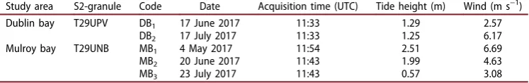
Another aspect to be taken into account in the selection of this processor is that C2RCC seems to reduce the sunglint present in the images; which does not happen when using the ACOLITE, iCOR or Sen2Cor processors. This fact could contribute to the relatively highR2values obtained with this processor. The presence of sunglint after the application of C2RCC was visually evaluated (Figure 3). Besides, the relationship between each visible band (B2–497 nm, B3–560 nm and B4–665 nm) considered in this study

and the NIR band (B8a–865 nm) was checked in areas of deep water not influenced by

the seafloor. All the images presented low correlation values after C2RCC application with an average ofR2= 0.24 for B2(497 nm),R2= 0.08 for B3(560 nm) andR2= 0.09 for

B4(665 nm). The decrease in these values in comparison with the original image can be

considered an indication of sunglint reduction that supports the visual evaluation. Although alternative sunglint correction methods have been described in the biblio-graphy (e.g. Hedley, Harborne, and Mumby2005; Kay, Hedley, and Lavender2009) they were not considered here as they would add an extra step to the processing chain. The results produced by C2RCC are considered reasonable for the purpose of this study.

3.2. Relation of satellite bands and in situ water depth

The relationships between bands after atmospheric correction using C2RCC were eval-uated. In case of considering a single band, B3(560 nm), representing the green region

of the electromagnetic spectrum, was the band that showed the strongest negative correlation with in situdepth in all cases, withr ranging between−0.81 and−0.87. B2

(497 nm) and B4 (664 nm) corresponding with the blue and red part of the

electro-magnetic spectrum presented moderate negative correlations with in situ depth, ran-ging theirrvalues for B2between−0.52 and−0.74 and for B4between−0.45 and−0.63. Table 2.Comparison ofR2betweenin situdepth and the log-transformed B2/B3band ratio using the different atmospheric correction (AT) processors: ACOLITE (AC), iCOR, Sen2Cor (S2C) and the Case 2 Regional CoastColour (C2RCC).

Study area Code Date AT R2 AT R2 AT R2 AT R2

Dublin bay DB1 17 June 2017 AC 0.68 iCOR 0.58 S2C 0.04 C2RCC 0.64

DB2 17 July 2017 AC 0.62 iCOR 0.73 S2C 0.48 C2RCC 0.64

Mulroy bay MB1 4 May 2017 AC 0.33 iCOR 0.73 S2C 0.57 C2RCC 0.77

MB2 20 June 2017 AC 0.08 iCOR 0.42 S2C 0.35 C2RCC 0.76

The linear relationship between different combinations of band ratios and in situ depth was also assessed. The widely used blue-green band ratio, B2 (497 nm)/B3

(560 nm) and B1 (444 nm)/B3 (560 nm), was the one that showed the strongest

correlation values. However, the ratio containing B1(444 nm) was ruled out due to the

coarse spatial resolution of this band (60 m). Therfor the B2(497 nm)/B3(560 nm) ratio,

considering the five Sentinel images, ranged between 0.80 and 0.88. Similar results,r values between−0.84 and−0.87, were found for the ratio of green and near-infrared red bands, B3(560 nm)/B8(833 nm). In Mulroy Bay, this band ratio, B3(560 nm)/B8(833 nm),

presented slightly weaker correlations than the B2(497 nm)/B3(560 nm). Correlations for

B2(497 nm)/B3(560 nm) were stronger in Mulroy Bay.

3.3. Assessment of bathymetry models in Dublin Bay

Before building the definitive LBM, both options of calculating Xj were investigated using Equations (3) and Equation (6). The relationship between the explanatory variables (atmospherically corrected Sentinel-2 bands using C2RCC processor) andin situ depth (multibeam data) was evaluated using multiple linear regressionfitted through Ordinary Least Squares (OLS). Theoretically the larger the number of bands employed, the larger of variations that can be tolerated (Lyzenga, Malinas, and Tanis2006). All possible band combinations were investigated, where the regression with the highest adjusted R2 coupled with the lowest collinearity (via VIF values) was obtained for a regression informed by bands B2(497 nm), B3(560 nm) and B4(665 nm).

The results of both variations for the calculation of Xjare presented in Table 3. The models with the highest adjusted R2 and lowest AIC were obtained for Xj without subtracting deep water values; however, the VIFs were highest in these models indicat-ing a higher redundancy between bands. For this reason, the inclusion of deep area values in the calculation ofXjwas considered (Equation (3)) and from now on the results presented will be referred to this variation.

Bathymetric maps using the LBM and the BRM for Dublin Bay are given inFigure 4. Of special attention is the striping effect caused by the alternation of detectors in the along-track direction of the MSI. This effect is nominal in Sentinel-2 imagery and is amplified when the levels of illumination from the sun are strongest on the eastern side of the image swath. The visual analysis of the resulting maps using LBM and BRM showed qualitatively good agreement with the charts produced by the INFOMAR programme using multibeam data. However, compared to the LBM, the BRM ratio model showed more spatially noisy results and saturated at estimated depths higher than 10 m. The LBM and BRM maps showed a progressive increase in depth from the shore to more external areas of the bay as described in other studies (e.g. Monteys et al.

2015). The LBM indicated a difference in depth between northern and southern areas being the areas at the northern bank of the Liffey River, close to the Howth peninsula, shallower. The Liffey River channel is clearly defined in the bathymetric maps as a deeper area. The Burford and Kish Banks are also detected by the models. These areas correspond to shallower sandbanks with an elongated shape that arise from horizontal plains of sediment ranging from gravel tofine sand. Both images, DB1and DB2, and both

models presented negative values in shallow areas close to the shore. These areas corresponded with depth values under 1 m and where bottom and floating material can influence the signal. An accumulation of seaweeds close to the shore can be appreciated in these areas in the Red Green Blue (RGB) composition.

To better describe the ability of the LBM and the BRM tofit the empirical data several statistics were evaluated (Table 4). In both images of Dublin Bay, DB1and DB2, the LBM

showed higherR2and lower RMSE and Bias values when the total number of validation points from 0 m to 10 m are considered, indicating this model to perform better than the BRM. The results were slightly better for the image taken on the 17 July 2017 (DB2).

When different depth ranges were analysed (0 m–2 m, 2 m–6 m, 6 m–10 m) both models showed the same trend. In general, the LBM provided the highest R2 values, lowest RMSE, and lowest Bias. Only in the depth range between 0 m and 2 m the Bias values were lower in the BRM. As the LBM is considered to perform generally better, we will focus only on these results from now on. Thus, when all ranges of depth are considered the LBM showed the highest R2 and lowest RMSE values, in the depth

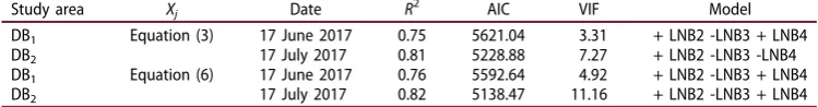
Table 3.Linear Band Model (LBM)fit assessment of the method forXjcalculation using Equations (3) and Equation (6). The different variables correspond to the Sentinel-2 bands after atmospheric correction using C2RCC processor. All variables included in the models showed apvalue = 0.01.

Study area Xj Date R2 AIC VIF Model

DB1 Equation (3) 17 June 2017 0.75 5621.04 3.31 + LNB2 -LNB3 + LNB4

DB2 17 July 2017 0.81 5228.88 7.27 + LNB2 -LNB3 -LNB4

DB1 Equation (6) 17 June 2017 0.76 5592.64 4.92 + LNB2 -LNB3 + LNB4

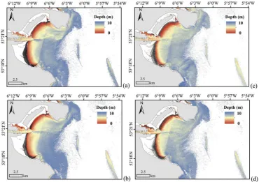
Figure 4.Bathymetric maps derived for Dublin Bay using: (a) Linear Band Model (LBM) for the image registered on the16 June 2017 (DB1) and (b) LBM for the image registered on the 17 July 2017 (DB2) (c) Log-transformed Band Ratio Model (BRM) for DB1and (d) BRM for DB2. The white areas close to the shore indicate the intertidal zone (0 m depth). The black areas correspond with negatives values.

Table 4._R2_{, RMSE, and Bias between measured water depths and satellite modelled depths for the} Linear Band Model (LBM) and the Log-transformed Band Ratio Model (BRM) at different depth ranges in Dublin Bay (DB). N represents the total number of validation points. In brackets the number of outliers. LBM and BRM were applied to atmospherically corrected Sentinel-2 data using the C2RCC processor.

Model Code Date Depth range (m) R2 _{Bias RMSE N}

Linear Band Model (LBM) DB1 17 June 2017 0–2 0.265 −0.534 0.852 164

2–6 0.828 −0.824 0.937 595 6–10 0.325 0.595 1.286 890 Total 0.835 −0.030 1.132 1649 DB2 17 July 2017 0–2 0.401 −0.648 0.932 164

2–6 0.547 −0.515 0.880 595 6–10 0.519 0.460 1.057 888 Total 0.873 −0.003 0.984 1647 (2) Log-transformed Band Ratio Model (BRM) DB1 17 June 2017 0–2 0.304 −0.163 1.038 164

2–6 0.531 −1.171 1.381 595 6–10 0.104 0.916 1.561 890 Total 0.720 0.056 1.453 1649 DB2 17 July 2017 0–2 0.242 −0.377 1.155 164

range between 2 m and 6 m. In both images, Bias was negative for depth ranges 0 m– 2 m and 2 m–6 m, indicating that the satellite-derived model overestimates the values at these depths. Bias was positive in the depth range 6 m–10 m, indicating that the satellite-derived model underestimates the values at these depths.

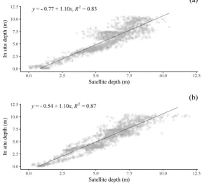
The scatterplots resulting from the LBM are given in Figure 5. Both showed over-estimation of satellite-derived depth at values shallower than 2 m and an underestima-tion of these values in areas deeper than 10 m. The overestimaunderestima-tion of modelled depths in areas shallower than 2 m was more acute in the DB1image while the underestimation

in the range of 6 m–10 m was more pronounced in DB2image. The tide height in both

images was very similar involving that these differences cannot be attributable to this fact.

3.4. Assessment of bathymetry models in Mulroy Bay

Before building the definitive LBM, both options of calculating Xj were investigated through Equation (3) and Equation (6) using the same process as in the case of Dublin Bay. The highest adjusted R2 and lowest AIC were obtained forXjwithout subtracting deep water values; however, the VIFs were highest in these models indicating a higher redundancy between bands (Table 5). For this reason, Equation (3) was preferred in the calculation ofXj. All possible band combinations were investigated, where the regression with the highest adjusted R2 coupled with the lowest collinearity (via VIF values) was

obtained for a regression informed by B2(497 nm), B3(560 nm) and B4(665 nm). All

bands were significant in all models (p values < 0.01) except for B4 (664 nm) in MB3.

However, B4was retained in the model for MB3to maintain consistency with the rest of

the images.

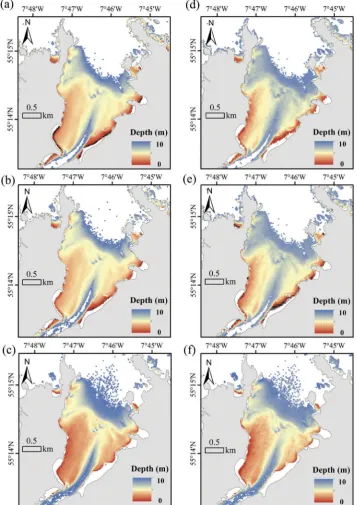
LMB and BRM were applied to the appropriate images to produce bathymetric maps (Figure 6). A visual inspection showed qualitatively good agreement with the charts produced by the INFOMAR programme using multibeam data and previous studies carried out in the area (Cahalane, Hanafin, and Monteys 2017). Shallow areas were located close to the shore, with the western side deeper than the eastern side. The deepest values were located at the mouth of the bay and at the inner channel. Negative values resulted in very shallow waters after the application of both models except for MB3, which is the image with the lowest tide (0.57 m). The areas of negative values were

larger in the bathymetric maps resulting from the BRMs.

LBM model presented higher R2and lower RMSE values than the BRM when all the validation points (0 m–10 m) were considered (Table 6). Due to the topography of the bay, the number of outliers was higher in the case of Mulroy Bay than previously identified in Dublin Bay. These values were located close to the shoreline and over rocky shallow areas that are exposed at low tide. This issue may explain why the highest number of outliers were found in MB3, as this image was captured at the lowest tide.

Bias values were lower for the LBM in all depth ranges considered except for the shallow areas (0 m–2 m). In this case, the BRM showed lower values.

As the LBM showed better fit than the BRM, it was chosen as the preferred model. Considering only the performance of this model in the three images, again high R2 values were found, as in the case of Dublin Bay, for the depth range between 2 m and 6 m. However, unlike Dublin Bay, high R2values were also found at depths between 6 m and 10 m, but in this case, the RMSE and Bias were higher. R2 values decreased considerably in the depth range 0 m–2 m. In MB1 and MB2, Bias values were negative

in the depth ranges 0 m–2 m and 2 m–6 m indicating an overestimation of the satellite-derived depth while these values were positive at depths higher than 6 m indicating an underestimation of satellite-derived values. In the case of MB3, the image registered in

the lowest tide, the trend is the same except for the range 0 m–2 m were Bias values were positive.

The LBM scatterplots confirm these results showing overestimation of satellite-derived depth at values shallower than 2 m and an underestimation of these values in areas deeper than 10 m (Figure 7). Modelled derived depths in areas shallower than 2 m

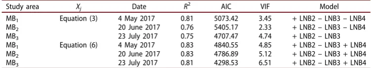
Table 5.Linear Band Model (LBM)fit: assessment of the method forXjcalculation using Equation (3) and Equation (6). The different variables correspond to the Sentinel-2 bands after atmospheric correction using C2RCC processor. All the models incorporated the three variables: B2, B3and B4. However, only variables that showed apvalue = 0.01 are included in the table.

Study area Xj Date R2 AIC VIF Model

MB1 Equation (3) 4 May 2017 0.81 5073.42 3.45 + LNB2–LNB3–LNB4

MB2 20 June 2017 0.76 5405.17 2.33 + LNB2–LNB3–LNB4

MB3 23 July 2017 0.75 4707.47 4.74 + LNB2–LNB3

MB1 Equation (6) 4 May 2017 0.83 4840.55 4.85 + LNB2–LNB3 + LNB4

MB2 20 June 2017 0.83 4786.89 5.12 + LNB2–LNB3 + LNB4

showed a high number of zero values in MB3as this image was registered in the lowest

tide (0.57 m).

4. Discussion

4.1. Atmospheric correction

As has been reported in many coastal studies (e.g. Lavender and Nagur2002; Casal et al.

2011; Vanhellemont and Ruddick 2015; Pahlevan, Roger, and Ahmad 2017b) atmo-spheric correction is critical in aquatic environments. The aim of this study was not to conduct an exhaustive comparison of atmospheric correction processors but to con-tribute to their evaluation in Irish waters, with the specific purpose of bathymetric applications. In our study, four atmospheric corrections: Sen2Cor version 2.4, ACOLITE, iCOR, and C2RCC were compared through their ability to produce linear relationships between ratios of log-transformed bands and depth, as the degree of light attenuation in the water column is wavelength dependent.

The different processors showed variable results among the images. Something to consider to justify this variability is the difference between the outputs produced by each processor. Processors such as ACOLITE and C2RCC produce remote sensing refl ec-tances while in the case of Sen2Cor and iCOR the outputs contain BOA reflectances that

Table 6._R2_{, RMSE, and Bias between measured water depths and modelled depths for the Linear} Band Model (LBM) and the Log-transformed Band Ratio Model (BRM) at different depth ranges in Mulroy Bay (MB). N represents the total number of validation points. In brackets the number of outliers. LBM and BRM were applied to atmospherically corrected Sentinel-2 data using the C2RCC processor.

Model Code Date

Depth range

(m) R2 _{Bias RMSE N}

Linear Band Model (LBM) MB1 4 May 2017 0–2 0.114 −0.364 0.992 80

2–6 0.681 −0.241 0.627 956 6–10 0.751 0.559 0.925 738

Total 0.885 0.086 0.782 1774 (23) MB2 20 June 2017 0–2 0.169 −0.342 1.012 75

2–6 0.688 −0.352 0.659 954 6–10 0.694 0.638 1.071 738

Total 0.856 0.062 0.870 1767 (23) MB3 23 July 2017 0–2 0.046 0.819 0.975 74

2–6 0.665 −0.237 0.751 941 6–10 0.774 0.392 0.782 743

Total 0.880 0.074 0.775 1758 (85) Log-transformed Band Ratio Model

(BRM)

MB1 4 May 2017 0–2 0.090 0.439 1.511 79

2–6 0.709 −0.359 0.817 958 6–10 0.669 0.573 1.060 745

Total 0.816 0.066 0.964 1782 (15) MB2 20 June 2017 0–2 0.056 0.614 1.272 81

2–6 0.199 0.030 1.125 106 6–10 0.799 0.085 0.931 1601

Total 0.819 0.107 0.963 1788 (9) MB3 23 July 2017 0–2 0.032 0.948 1.000 83

include sunglint and whitecaps contributions. As it was expected, Sen2Cor produced the lowest correlations due to it was initially designed for terrestrial areas and does not take into account intrinsic characteristics of the water column. ACOLITE was designed for turbid waters, and this can explain thatR2were higher in Dublin Bay, that presents more optically complex waters than Mulroy Bay as it was mentioned in the description of the study areas. In the case of iCOR,R2 were high in some of the images but these high values were not consistent in the whole dataset. The output of iCOR consists of BOA reflectances and sunglint can be appreciated after the application of this processor. A possible justification of the low values in some of the images can be the presence of sunglint not homogeneously distributed.

The processor that showed the highest and the most consistentR2values in all the images was the C2RCC processor. C2RCC was developed for Case 2 waters and relies on a large database of simulated water leaving reflectances and related TOA radiances (Bockmann et al.2016). The conditions of our study areas seem to be represented in this large database as C2RCC provided the highest R2 values. The important reduction of sunglint by this processor could be the final responsible of these high values. As mentioned before although alternative sun glint correction methods exist they were not considered as the C2RCC provided reasonable results for the purpose of this study reducing in one step the processing chain. A more exhaustive comparison of ACOLITE,

Figure 7.Scatterplot of satellite-derived depth versus the multibeam in situ depth using the linear band model (LBM) for (a) MB1(b) MB2and (c) MB3. The black line indicates the 1:1 ideal line of best

iCOR with C2RCC, applying sunglint correction if necessary, need to be considered for a more comprehensive evaluation on the performance of these processors over aquatic environments.

4.2. Assessment of bathymetric models

While in clear waters the blue band should be selected for bathymetry retrieval due to its higher penetration into the water column, in turbid waters the optimal bands shift to longer wavelengths such as green-yellow spectral regions (Vahtmäe and Kutser2016). This was in part confirmed in both of our study areas where the green band (560 nm) showed the highest correlation coefficients with water depth followed by the blue band (497 nm). The LBM applied to the Sentinel-2 data showed a betterfit to thein situbathymetry data in all the analysed images in comparison to BRM. These results are in concordance with other works carried out in turbid waters that reported the samefindings (Lyons, Phinn, and Roelfsema 2011; Bramante, Raju, and Sin 2013; Ehnes and Rooney 2015; Vahtmäe and Kutser 2016). In our case, this model considers three different bands instead of two used in the log-transformed band ratio model. The higher number of bands may provide more information about the water column and bottom conditions and so contribute to the better results. A closerfit of the satellite-derived bathymetry to the in situ bathymetry was reached, in general, for Mulroy Bay. This result can be explained because of the different water column conditions in both study areas, where Mulroy Bay has higher water transparency. Another aspect to consider here in the different spatial distributions of the calibration data. In the case of Dublin Bay, the calibration data are sparse as result of the vessel transects while in Mulroy Bay is homogeneous covering all bottom types and water quality conditions. This issue could also be responsible of the higherR2values obtained in Mulroy Bay.

Bathymetric maps showed consistence between dates in both study areas as the images were registered within less than one year between them. This reinforces the potential of Sentinel-2 data at longer time scales for monitoring purposes in the Irish coast. In both study areas, the highestR2and lowest RMSE values were obtained when the depth range was restricted to being between 2 m and 6 m. These areas of the water column are considered to be more stable without bottom influence and the loss of correlation between reflectance and depths higher than 6 m. In both study areas, some negative values appeared close to the shoreline except for MB3which was registered in

the lowest high tide. This could be explained by the influence of the bottom signal in areas shallower than 2 m. This issue would be especially important in Dublin Bay, where blooms of green algae in the intertidal area and subtidal blooms of the brown algae Ectocarpus siliculosusare registered (Jeffrey et al.1995). Algae and rocky bottoms present a darker signal compared to deep water areas having an influence on the performance of the model (Casal et al.2013; Vahtmäe and Kutser2016).

The alternation of detectors in the Sentinel-2 MSI affects the study area of Dublin Bay. However, even only two images were evaluated (due to cloud coverage conditions), the influence of this effect was actually small in the bathymetric profiles (Figure 8). In the case of Dublin Bay, there is a difference between bathymetric profiles (Figure 8 (b) and (c)) that could be explained by the different water quality conditions. In the case of DB2, a more

windy conditions present when the image was registered could contribute to the resuspen-sions of suspended material that can have an influence on the performance of the models. The selection of optimal images or the use of models that can handle variation in the bottom and water quality conditions are essential in the extraction of satellite-derived bathymetry.

TheR2values obtained in this study were similar to the ones obtained in studies that applied the same empirical methods to sensors of higher spatial resolution (e.g. Lyons, Phinn, and Roelfsema 2011; Hamylton, Hedley, and Beaman 2015: Hernández and Armstrong2016) indicating that empirical models applied to Sentinel-2 data can provide a good correspondence with bathymetry (Figure 8). The study carried out by Monteys et al. (2015) in the same study area of Dublin Bay reported higherR2values using spatial prediction methods in a single image of RapidEye (5 m per pixel). Although both studies are not comparable because of the different sensors with different technical character-istics, Monteys et al. reported higher accuracies when models that account for spatial effects are used. This suggests spatial regression models may offer some advantages. Nevertheless, this study demonstrates that LBMs are a reasonable starting point when the images are taken in optimal conditions (e.g. water clarity, no wind).

5. Conclusions and future work

Even further analyses are required, this study suggests that Sentinel-2 data can be a good alternative to cover the unmapped areas in the Irish coast. Atmospheric correction and bottom reflectance as well as water quality conditions were proved to be critical factors in thefit of the bathymetric models. Results showed that LBMs provide betterfit to empirical data than the BRM in the both study areas considered in this study. Future work using spatially explicit predictive models and physics-based analytical approaches will be done to optimise Sentinel-2 bathymetry derivation in the Irish coast.

Acknowledgements

This study was carried out as part of the projectOptical Remote Sensing for bathymetry and seabed

mapping in the coast of Ireland (BasMaI). BaSMaI is supported by the Geological Survey Ireland/

DCCAE Postdoctoral Fellowship Programme under the grant No. 2016-PD-005. Multibeam data were provided by INFOMAR Programme. Tide data were obtained through the Irish National Tide Gauge Network. ESA and Copernicus are thanked for Sentinel-2A imagery. Authors would like to thank the three anonymous reviewers for their helpful comments and suggestions.

Disclosure statement

No potential conflict of interest was reported by the authors.

Funding

ORCID

Paul Harris http://orcid.org/0000-0003-0259-4079

References

Bockmann, C., R. Doerffer, M. Peters, K. Stelzer, S. Embacher, and A. Ruescas.2016.““Evolution of the C2RCC Neural Network for Sentinel 2 and 3 for the Retrieval of Ocean Colour Products in Normal and Extreme Optically Complex Waters”.”InProceedings of the Living Planet Symposium 2016. Prague, Czech Republic. 9-13 May 2016

Bramante, J. F., D. K. Raju, and T. M. Sin. 2013. “Multispectral Derivation of Bathymetry in Singapore’s Shallow, Turbid Waters.” International Journal of Remote Sensing 34 (6): 2070– 2088. doi:10.1080/01431161.2012.734934.

Brando, V. E., J. M. Anstee, M. Wettle, A. G. Dekker, S. R. Phinn, and C. Roelfsema.2009.“A Physics Based Retrieval and Quality Assessment of Bathymetry from Suboptimal Hyperspectral Data.”

Remote Sensing of Environment113:755–770.

Brooks, P. R., R. Nairn, M. Harris, D. Jeffrey, and T. P. Crowe.2016.“Dublin Port and Dublin Bay: Reconnecting with Nature and People.” Regional Studies in Marine Science 8: 234–251. doi:10.1016/j.rsma.2016.03.007.

Cahalane, C., J. Hanafin, and X. Monteys. 2017. “Improving Satellite-Derived Bathymetry Using Spatial Regression Algorithms.”Hydro International, 16–19.

Casal, G., T. Kutser, J. A. Domínguez-Gómez, N. Sánchez-Carnero, and J. Freire. 2011.“Mapping Benthic Macroalgal Communities in the Coastal Zone Using CHRIS-PROBA Mode 2 Images.”

Estuarine, Coastal and Shelf Science94 (3): 281–290. doi:10.1016/j.ecss.2011.07.008.

Casal, G., T. Kutser, J. A. Domínguez-Gómez, N. Sánchez-Carnero, and J. Freire.2013.“Assessment of the Hyperspectral Sensor CASI-2 for Macroalgal Discrimination on the Ria De Vigo Coast (NW Spain) Using Field Spectroscopy and Modelled Spectral Libraries.”Continental Shelf Research55: 129–140. doi:10.1016/j.csr.2013.01.010.

Chust, G., M. Grande, I. Galparsoro, A. Uriarte, and A. Borja.2010.“Capabilities of the Bathymetric Hawk Eye LiDAR for Coastal Habitat Mapping: A Case Study within A Basque Estuary.”Estuarine,

Coastal and Shelf Science84 (4): 200–213. doi:10.1016/j.ecss.2010.07.002.

Chybiki, A. 2017.“Mapping South Baltic Near-Shore Bathymetry Using Sentinel-2 Observations.”

Polish Maritime Research3 (95): 24–25.

Coveney, S., and X. Monteys.2011.“Integration Potential of INFOMAR Airborne LIDAR Bathymetry with External Onshore LIDAR Data Sets.”Journal of Coastal Research 62: 19–29. doi:10.2112/ SI_62_3.

Dekker, A. G., S. R. Phinn, J. Anstee, P. Bissett, V. E. Brando, B. Casey, P. Fearns, et al. 2011. “Intercomparison of Shallow Water Bathymetry, Hydro-Optics, and Benthos Mapping Techniques in Australian and Caribbean Coastal Environment.” Limnology and Oceanography:

Methods9: 396–425.

Doerffer, R., and H. Schiller. 2007.“The MERIS Case 2 Water Algorithm.”International Journal of

Remote Sensing28 (3): 517–535. doi:10.1080/01431160600821127.

Ehnes, J. S., and J. J. Rooney. 2015. “Depth Derivation Using Multispectral WorldView-2 Satellite

Imagery”. U.S.Department of Commerce, NOAA Technical Memorandum NMFS-PIFSC-46.

Honolulu, Hawaii.

Eugenio, F., J. Marcello, J. Martin, and J. G. Rodŕıguez-Esparragón.2017.“Benthic Habitat Mapping Using Multispectral High-Resolution Imagery: Evaluation of Shallow Water Atmospheric Correction Techniques.”Sensors17: 2639. doi:10.3390/s17050968.

Gordon, H. R., and A. Y. Morel. 1983.“Remote Assessment of Ocean Color for Interpretation of Satellite Visible Imagery.”InA Review of Lecture Notes on Coastal and Estuarine Studies, 114. New York: Springer-Verlag.

Guanter, L.2007.“New algorithms for atmospheric correction and retrieval of biophysical para-meters in earth observation. Application to ENVISAT/MERIS data”. PhD diss., Universidad de Valencia.

Hamylton, S. M., J. D. Hedley, and R. J. Beaman.2015.“Derivation of High-Resolution Bathymetry from Multispectral Satellite Imagery: A Comparison of Empirical and Optimisation Methods through Geographical Error Analysis.”Remote Sensing7: 16257–16273. doi:10.3390/rs71215829. Hedley, J., A. R. Harborne, and P. J. Mumby.2005.“Simple and Robust Removal of Sun Glint for Mapping Shallow-Water Benthos.” International Journal of Remote Sensing 26: 2107–2112. doi:10.1080/01431160500034086.

Hedley, J., C. Roelfsema, B. Koetz, and S. Phinn.2012.“Capability of Sentinel-2 Mission for Tropical Coral Reef Mapping and Coral Bleaching Detection.”Remote Sensing of Environment120: 145– 155. doi:10.1016/j.rse.2011.06.028.

Hedley, J., C. Roelfsema, V. Brando, C. Giardino, T. Kutser, S. Phinn, P. Mumby, O. Barrilero, J. Laporte, and B. Koetz. 2018.“Coral Reef Applications of Sentinel-2: Coverage, Characteristics, Bathymetry and Benthic Mapping with Comparison to Landsat 8.” Remote Sensing of

Environment216: 598–614. doi:10.1016/j.rse.2018.07.014.

Hernández, W. J., and R. A. Armstrong. 2016.“Deriving Bathymetry from Multispectral Remote Sensing Data.”Journal of Marine Science and Engineering4 (1): 8. doi:10.3390/jmse4010008. IOCCG. 2010. Atmospheric Correction for Remotely-Sensed Ocean-Colour Products”.Reports of

the International Ocean-Colour Coordinating Group, No. 10, IOCCG, edited by M. Wang, 78.

Dartmouth, Canada. doi:10.25607/OBP-101.

Jeffrey, D. W., B. M. Brennan, E. Jennings, B. Madden, and J. G. Wilson.1995.“Nutrient Sources for In-Shore Nuisance Macroalgae: The Dublin Bay Case.”Ophelia42:147–161.

Kabiri, K.2017.“Discovering Optimum Method to Extract Depth Information for Nearshore Coastal Waters from Sentinel-2A Imagery Case-Study: Nayband Bay, Iran.”The International Archives of the Photogrammetry, Remote Sensing and Spatial Information Sciences, Volume XLII-4/W4, edited by F. Karimipour and F. Samadzadegan. Tehran, Iran. October 7-10.

Kay, S., J. Hedley, and S. Lavender.2009.“Sun Glint Correction of High and Low Spatial Resolution Images of Aquatic Scenes: A Review of Methods for Visible and Near-Infrared Wavelengths.”

Remote Sensing1: 697–730. doi:10.3390/rs1040697.

Lavender, S., and C. R. C. Nagur.2002.“Mapping Coastal Waters with High Resolution Imagery: Atmospheric Correction of Multi-Height Airborne Imagery.”Journal of Optics A: Pure and Applied

Optics4 (S50): S55. doi:10.1088/1464-4258/4/4/363.

Legleiter, C. J., D. A. Roberts, W. A. Marcus, and M. A. Fonstad. 2004.“Passive Optical Remote Sensing of River Channel Morphology and In-Stream Habitat: Physical Basis Feasibility.”Remote

Sensing of Environment93: 493–510. doi:10.1016/j.rse.2004.07.019.

Liu, H., Q. Li, T. Shi, S. Hu, G. Wu, and Q. Zhou.2017.“Application of Sentinel 2 MSI Images to Retrieve Suspended Particulate Matter Concentrations in Poyang Lake.”Remote Sensing9: 761. doi:10.3390/rs9070761.

Louis, J., V. Debaecker, B. Pflug, and M. Main-Knorn.2016. Sentinel-2 Sen2Cor: L2A Processor for Users. In Proceedings of the Living Planet Symposium. Prague, Czech Republic, 9-13 May 2016. Lyons, M., S. Phinn, and C. Roelfsema.2011.“Integrating Quickbird Multis-Pectral Satellite and Field Data: Mapping Bathymetry, Seagrass Cover, Seagrass Species and Change in Moreton Bay, Australia in 2004 and 2007.”Remote Sensing3 (1): 42–64. doi:10.3390/rs3010042.

Lyzenga, D. R.1978.“Passive Remote Sensing Techniques for Mapping Water Depth and Bottom Features.”Applied Optics17: 379–383.

Mansfield, M. 1992.“Dublin Bay Water Quality Management Plan: Field Studies of Currents and Dispersion”. Technical Report 3, Environmental Research Unit, Ireland.

Monteys, X., P. Harris, S. Caloca, and C. Cahalane.2015.“Spatial Prediction of Coastal Bathymetry Based on Multispectral Satellite Imagery and Multibeam Data.”Remote Sensing7: 13782–13806. doi:10.3390/rs71013782.

Moreno-Navas, J., T. C. Telfer, and L. G. Ross.2011.“Application of 3D Hydrodynamic and Particle Tracking Models for Better Environmental Management of Finfish Culture.”Continental Shelf

Research31: 675–684. doi:10.1016/j.csr.2011.01.001.

O’Boyle, S., and J. Silke.2010.“A Review of Phytoplankton Ecology in Estuarine and Coastal Waters around Ireland.”Journal of Plankton Research32 (1): 99–118. doi:10.1093/plankt/fbp097. O’Higgins, T. G., and J. G. Wilson. 2005. “Impact of the River Liffey Discharge on Nutrient and

Chlorophyll Concentrations in the Liffey Estuary and Dublin Bay (Irish Sea).”Estuarine, Coastal

and Shelf Science64: 323–334. doi:10.1016/j.ecss.2005.02.025.

Pahlevan, N., J. C. Roger, and Z. Ahmad.2017b.“Revisiting Short-Wave-Infrared (SWIR) Bands for Atmospheric Correction in Coastal Waters.” Optics Express 25 (6): 6015–6034. doi:10.1364/ OE.25.006015.

Pahlevan, N., S. Sarkar, B. A. Franz, S. V. Balasubramanian, and J. He.2017a.“Sentinel-2 MultiSpectral Instrument (MSI) Data Processing for Aquatic Science Applications: Demonstrations and Validations.”Remote Sensing of Environment201: 47–56. doi:10.1016/j.rse.2017.08.033.

Salama, M., M. Radwan, and R. van der Velde.2012.“A”Hydro-Optical Model for Deriving Water Quality Variables from Satellite Images (Hydrosat): A Case Study of the Nile River Demonstrating the Future Sentinel-2 Capabilities”.” Physics and Chemistry of the Earth 50-52: 224–232. doi:10.1016/j.pce.2012.08.013.

Sterckx, S., E. Knaeps, S. Adriaensen, I. Reusen, L. De Keukelaere, and P. Hunter.2015a.“Opera: An Atmospheric Correction for Land and Water”. In Proceedings of the ESA Sentinel-3 for Science

Workshop. Venice, Italy. 2-5 June 2015. ESA SP-734.

Sterckx, S., S. Knaeps, S. Kratzer, and K. Ruddick.2015b.“SIMilarity Evnironment Correction (SIMEC) Applied to MERIS Data over Inland and Coastal Waters.”Remote Sensing of Environment157: 96– 110. doi:10.1016/j.rse.2014.06.017.

Stumpf, R. P., K. Holderied, and M. Sinclair. 2003. “Determination of Water Depth with High-Resolution Satellite Imagery over Variable Bottom Types.” Limnology and Oceanography 48: 547–556. doi:10.4319/lo.2003.48.1_part_2.0547.

Telfor, T., and K. Robinson.2003.“Environmental Quality and Carrying Capacity for Aquaculture.”In

Marine Environmental and Health Series, No. 9, edited by M. B. Co and Donegal. Ireland: Marine

Institute. ISSN: 1649-0053.

Toming, K., T. Kutser, A. Laas, M. Sepp, B. Paavel, and T. Nõges.2016.“First Experiences in Mapping Lake Water Quality Parameters with Sentinel-2 MSI Imagery.” Remote Sensing 8: 640. doi:10.3390/rs8080640.

Traganos, D., D. Poursanidis, B. Aggarwal, N. Chrysoulakis, and P. Reinartz. 2018. “Estimating Satellite-Derived Bathymetry (SDB) with the Google Earth Engine and Sentinel-2.” Remote

Sensing10: 859. doi:10.3390/rs10060859.

Vahtmäe, E., and T. Kutser.2016.“Airborne Mapping of Shallow Water Bathymetry in the Optically Complex Waters of the Baltic Sea.” Journal of Applied Remote Sensing 10 (2): 025012. doi:10.1117/1.JRS.10.025012.

Vanhellemont, Q., and K. Ruddick.2015.“Advantages of High Quality SWIR Bands for Ocean Colour Processing: Examples from Landsat-8.”Remote Sensing of Environment161: 89–106. doi:10.1016/ j.rse.2015.02.007.