Coherence and path indistinguishability for the interference of
multiple single-mode fields
Rathindra Nath Das∗
Department of Physics, Indian Institute Technology Bombay,
Powai, Mumbai, Maharashtra 400076
Sobhan Kumar Sounda†
Department of Physics, Presidency University, 86, 1,
College St, College Square, Kolkata, West Bengal 700073
(Dated: August 10, 2020)
Abstract
A well known result for the interference of two single-mode fields is that the degree of coherence
and the degree of indistinguishablity are same when we consider the detection of a single photon.
In this article we present the relation between degree of coherence, path indistinguishability and
the fringe visibility considering interference of multiple number of single-mode fields while being
interested in the detection of a single photon only . We will also mention how Born’s rule of
I. INTRODUCTION
The equivalence of coherence and indistinguishability is an very important result in the
perspective of wave-particle duality. Coherence is one of the main criteria for interference of
light beams. On the other hand in single photon interference experiment the lack of photon’s
path information plays a crucial role. In his famous article L. Mandel1 has shown that the
modulus of degree of second order coherence is identical to the degree of indistinguishability
for the case of two single-mode fields emitted from two sources and by considering the
detection a single photon only. In recent times experiments of interference for more than
two slits2 has been of prime interest for proving the validity of Born’s rule . In this paper we describe the generalisation of L. Mandel’s result for 3 single-mode fields followed by N
number of single-mode fields while considering the detection of a single photon only. We
also discuss how the equivalent form of Born’s rule is obtained in the context of coherence
and fringe visibility.
II. INTERFERENCE OF THREE SINGLE-MODE FIELDS
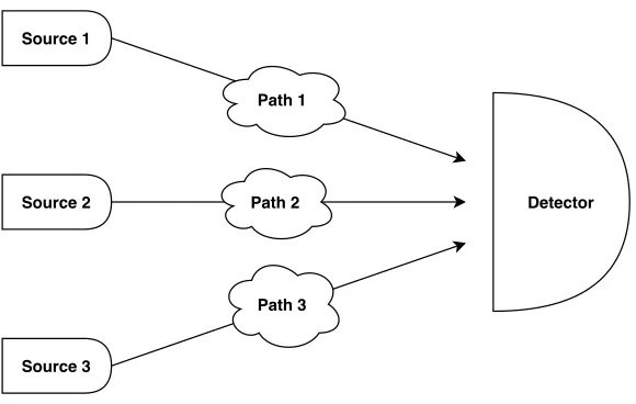
Before we discuss the generalised version of the interference, We consider the case of
interference of three single-mode fields and the detection of a single photon only. The
schematic diagram of the experiment under consideration is shown at Fig.1. Here we have
three sources and so a photon detected at any point on the detector may take three possible
paths. We write the state of the photon before the detection process takes place as
|ψi=α|1i1|0i2|0i3+β|0i1|1i2|0i3+γ|0i1|0i2|1i3 (1)
where|α|2,|β|2 and|γ|2are the probability of the photon being produced by the first, second
and third source respectively and |α|2+|β|2+|γ|2 = 1. Considering this state the density
matrix of this pure state can be written as
ˆ
ρID =|ψihψ|
=
|α|2 αβ∗ αγ∗
α∗β |β|2 βγ∗
α∗γ β∗γ |γ|2
Detector Source 1
Source 2
Source 3
Path 1
Path 2
Path 3
FIG. 1. Schematic diagram of the interference experiment
On the other hand we could have an incoherent mixture of states and the corresponding
density matrix of this photon represented by a diagonal density matrix of the form
ˆ ρD=
|α|2 0 0
0 |β|2 0
0 0 |γ|2
(3)
In the second case we do not have the off diagonal terms implying that the intrinsic
indistin-guishability of the photon path is lost. So, now for the density matrix ˆρD in principle we will
be able to detect the source of this photon experimentally and the interference pattern will
be lost. Following the notation of L. Mandel here also the subscript of ˆρID and ˆρD signifies
the path indistinguishability and this potential path distinguishability for those two density
matrices respectively. Now in this Hilbert space we take a general density matrix of the
form
ˆ ρ=
3
X
n,m=1
ρnm|nihm| (4)
and we can decompose it in the terms of ˆρID and ˆρD to determine the degree of
indistin-guishability for the system . We write the general density matrix as
ˆ
ρ=PIDρˆID+PDρˆD where PID+PD = 1 (5)
From Eq.5, Eq.4 and Eq.3 we get
ρ11 =|α|2, ρ22 =|β|2, ρ33=|γ|2 (6)
due to the hermiticity of the density matrix we can evaluate the lower triangular elements
as the complex conjugate of the upper triangular ones. Now using very simple calculation
we see that
PID = ρ12
√
ρ11ρ22
e−i·arg(ρ12) = √ρ13
ρ11ρ33
e−i·arg(ρ13) = √ρ23
ρ22ρ33
e−i·arg(ρ23) (8)
= √|ρ21|
ρ11ρ22
= √|ρ31|
ρ11ρ33
= √|ρ32|
ρ22ρ33
which indicates that PID can be written in three equivalent forms where we only have
pairwise terms out of the three slits.
Now we calculate the degree of coherence for the system and for that We denote the
positive frequency component of the single-mode electric field of the source as
ˆ
E(+)(rj) = Kˆaj where j = 1, 2, 3 (9)
. The normalised second order coherence function of the form3,4
g(1)(xi, xj) =
G(1)(x
i, xj) p
G(1)(x
i, xi)G(1)(xj, xj)
(10)
where
G(1)(xi, xj) = Tr{ρˆEˆ(−)(xi) ˆE(+)(xj)} (11)
and G(1)(xi, xj) is the general second order coherence function. For the first pair of sources (x1, x2) we get G(1)(x1, x2) of the form
G(1)(x1, x2) =T r{ρˆEˆ(−)(x1) ˆE(+)(x2)}
=|K|2ρ21 (12)
similarly we get,
G(1)(x1, x1) = |K|2ρ11 (13)
G(1)(x2, x2) = |K|2ρ22 (14)
Now from Eq.10,12,13 and 14 we get,
g(1)(x1, x2) =
ρ21
(ρ11ρ22)
1 2
We can do similar calculation for other pair of sources and we will get
g(1)(x1, x3) =
ρ31
(ρ11ρ33)
1 2
(16)
g(1)(x2, x3) =
ρ32
(ρ22ρ33)
1 2
(17)
Now from Eq.8, Eq.15, Eq.16 and Eq,17 we see that
PID=|g(1)(x1, x2)|, PID =|g(1)(x1, x3)| and PID =|g(1)(x2, x3)| (18)
So, we see that the degree of indistinguishability is equal to the degree of coherence even
for the case of interference with three sources but in a pair wise manner for all possible
combinations of two sources and we also note that the degree of coherence for all pairs of
sources are equal to each other.
Now it is very straight forward to show that only the second order normalised coherence
of this system is non zero. Any higher order coherence of the following form will be zero for
this system;
g(2)(xi, xj;xj, xi) =
G(2)(x
i, xj;xj, xi) p
G(1)(x
i, xi)G(1)(xj, xj) = 0
where G(2)(x
i, xj) = Tr{ρˆEˆ(−)(xi) ˆE(−)(xj) ˆE(+)(xj) ˆE(+)(xi)} is the general fourth order co-herence function4 or the three point fourth order coherence function
g(3)(xi, xj, xk;xk, xj, xi) =
G(3)(xi, xj, xk;xk, xj, xi) p
G(1)(x
i, xi)G(1)(xj, xj)G(1)(xk, xk) = 0.
So, we see that when we are interested in the detection of a single photon the modulus of
degree of indistinguishability and the degree of second order two point coherence will be
equal for all possible pairs of the three sources.
Now we look at the relation of fringe visibility with the degree of path indistinguishability
. For that we ignore the overall scaling and write the total positive component of electric
field at the point of detection as
ˆ
E(+) = ˆa1eiφ1+ ˆa2eiφ2 + ˆa3eiφ3 (19)
Here the phases φ1, φ2 and φ3 are acquired during the propagation of the field from source
to the point of detection. So, the probability of the photon being detected at this point is
Tr( ˆE(−)Eˆ(+)ρ) = Trˆ haˆ†1e−iφ1 + ˆa†
2e
−iφ2 + ˆa†
3e −iφ3
ˆ
a1eiφ1 + ˆa2eiφ2 + ˆa3eiφ3
ˆ ρi
where φij =φi−φj. The visibility of interference fringe is defined as3
V = Imax−Imin Imax+Imin
(21)
In Eq.20 the angle differenceφij can be varied to getImaxandImin. Then from Eq.15, Eq.16,
Eq.17 and Eq.21 we get
V = 2 (|ρ21|+|ρ31|+|ρ32|) ρ11+ρ22+ρ33
= 2
|g(1)(x1, x2)| (ρ11ρ22)
1
2 +|g(1)(x1, x3)| (ρ11ρ33) 1
2 +|g(1)(x2, x3)| (ρ22ρ33) 1 2
(22)
Using the inequality
2pI1I2 ≤ I1+I2 (23)
we can write
2√ρ11ρ22 ≤ρ11+ρ22 (24)
as ρii>0 for i=1,2,3 we can write Eq.24 as
2√ρ11ρ22 ≤ ρ11+ρ22+ρ33 = 1
√
ρ11ρ22 ≤
1
2 (25)
Similarly,
√
ρ11ρ33 ≤
1
2 and
√
ρ22ρ33 ≤
1
2 (26)
Using Eq.25 and Eq.26 in Eq.22 we get
V ≤ |g(1)(x1, x2)|+|g(1)(x1, x3)|+|g(1)(x2, x3)|
(27)
≤ (3PID) (28)
Here we see that the fringe visibility is related to the sum of modulus of two point coherence
functions for all three possible pairs of slits which is reminiscent of the famous Born’s rule
of multi-source interference. Very simple calculation shows how according to Born’s rule in
quantum mechanics, the multi-slit interference experiment’s fringe intensity is nothing but
the sum of contribution’s of all possible pairs of slits2. In that paper2 they experimentally
proved the validity of Born’s rule for three slit experiments that rules out the possibility of
III. COHERENCE AND INDISTINGUISHABILITY FOR INTERFERENCE WITH N SOURCES
Now we generalise our result for N sources where we are interested in detection of one
photon. For the generalisation of the problem we use a new notation for simplification of
the calculation. We denote the state |1i1⊗ |0i2⊗ |0i3 ⊗ |0i4..|0iN simply as ||1i. So when the photon will be generated by the m th source the state will be denoted as ||mi which in our old notation would be |0i1⊗ |0i2⊗ |0i3⊗...|1im⊗...|0iN and so on. So the state of the photon for this case can be written as
|ψi= N X
i=1
αi||ii (29)
where|αi|2 is the probability of the state ψ being in the i th state. Now for this the density matrix can be written as
ˆ
ρID =|ψihψ|= N X
i,j=1
αiα∗j||iihj|| (30)
and likewise we denote the diagonal form of the density as
ˆ ρD =
N X
i=1
αiα∗i||iihi||= N X
i=1
|αi|2||iihi|| (31)
Now any general density matrix can be written as
ˆ ρ=
N X
i,j=1
ρij||iihj|| (32)
Now by decomposing this density matrix in terms of the ρD and ρID we can write
ˆ
ρ=PIDρˆID+PDρˆD
=PID N X
i,j=1
αiα∗j||iihj||+PD N X
i=1
|αi|2||iihi|| (33)
= N X
i=1
|αi|2||iihi||+PID N X
i6=j=1;
αiαj∗||iihj|| (34)
Now by comparing Eq.34 and Eq.32 we can write
By hermiticity of density matrix we can write
ρji =ρ∗ij =PIDα∗iαj (36)
So, From Eq.35 and Eq.36 we can write,
ρijρji =PID2 ρiiρjj (37)
From Eq.35 and 37 we write
(αiα∗j)
2 = ρ 2
ij P2
ID
= ρ
2
ij ×ρiiρjj ρijρji
(38)
Due to hermiticity of density matrix
ρij =ρjie2i·arg(ρij) (39)
Using Eq.38, Eq.39 and Eq.35 we can get,
PID = ρij
√
ρiiρjj
e−i·arg(ρij) = √|ρij|
ρiiρjj
= √|ρji|
ρiiρjj
(40)
PID can be expressed in NC2 equivalent ways considering all possible pairs of N sources.
This result boils down to Eq.18 for N=3 case and L. Mandel’s result1 for N=2 case. Eq.40 suggests that the degree of path indistinguishability are equal for all possible NC
2 pairs of
sources.
Now to calculate the degree of coherence we denote the positive frequency part of the
single-mode electric fields of these sources as
ˆ
E(+)(rj) =Kˆaj where j = 1,2, ...N (41)
Now as we have N sources we will have NC
2 pairs of sources for which we can calculate the
second order coherence function. We calculate the general second order coherence function
for a pair of points (xi, xj) from Eq.10 and Eq.32 as
G(1)(xi, xj) =|K|2Tr(ˆa
†
iˆajρ) =ˆ |K|2 N X
n=1
hn||ˆa†iaˆjρˆ||ni
=|K|2
N X
n=1
hn||ˆa†iaˆj N X
l,k=1
ρlk||lihk|| !
||ni
=|K|2
N X
k,l=1
From Eq.42 and Eq.10 we see that
g(1)(xi, xj) = ρji
√
ρiiρjj
. (43)
We also note any higher order coherence function than this will be zero for this
gener-alised case also. From Eq.40 and Eq.43 one sees that these pairwise second order coherence
functions are equal to the modulus of degree of indistinguishability,
|g(1)(xi, xj)|=PID (44)
Therefore, for N single-mode fields when we consider the detection of a single photon
only we see that the degree of coherence is exactly equal to the modulus of degree of
indis-tinguishability when we consider all possible pairs of the sources. Now to relate degree of
indistinguishability with the degree of coherence we denote the total positive component at
the point of detection without the scaling factor as
ˆ E(+) =
N X
m=1
ˆ
ameiφm (45)
whereφnis the phase acquired by the field while propagating to the point of detection from
the n th source. We denote the intensity as well as the detection probability at this point
of detection as expectation of the operator ˆE(−)Eˆ(+) as
Tr
ˆ
E(−)Eˆ(+)ρ
= N X
i=1
ρii + 2 N X
i,j=1;i>j
|ρij| cos(φij) (46)
From Eq.21, Eq.23 and Eq.46 we write the visibility as
V = 2 N P
i,j=1;i>j
|ρij| N
P
i=1
|ρii|
= 2 N X
i,j=1;i>j
|g(1)(xi, xj)|(ρiiρjj)
1
2 wherei > j (47)
≤
N X
i,j=1;i>j
(|g(1)(xi, xj)|) (48)
≤ NC
2PID (49)
Eq.47 is the general form for interference fringe visibility of N single-mode fields. Eq.48 and
Eq.49 are the generalised relations between the fringe visibility , degree of coherence and
degree of indistinguishability. Here also as expected from the results of three fields we get
IV. CONCLUSION
In this article we present a generalised relations between degree of indistinguishability
and the degree of coherence. We also see how these quantities are related to the visibility of
interference fringe for N single-mode fields for detection of one photon only. We also note
the consistency of these results with Born’s rule for the interference fringe . These results
present a good picture or relations between wave and particle nature of photon.
1 L. Mandel, “Coherence and indistinguishability”, Opt. Lett. 16, 1882-1883(1991).
doi:10.1364/OL.16.001882
2 Urbasi Sinha, Christophe Couteau, Zachari Medendorp, Immo S¨ollner, Raymond Laflamme, Rafael
Sorkin, Gregor Weihs,“Testing Born’s Rule in Quantum Mechanics with a Triple Slit Experiment”,
AIP Conference Proceedings 1101, 200 (2009);. doi:10.1063/1.3109942
3 Max Born, Emil Wolf “Principles of Optics”,(1999). ISBN:9781139644181,
doi:10.1017/CBO9781139644181
4 Christopher Gerry, Peter Knight “Introductory Quantum Optics 1st Edition”,(2004).