Axial Diffusion of the Higher Order Scheme on the Numerical Simulation of Non-steady Partial Differential Equation in the Human Pulmonary Capillaries

Article

Axial Diffusion of the Higher Order Scheme on the

Numerical Simulation of Non-steady Partial

Differential Equation in the Human Pulmonary

Capillaries

Azim Aminataei and Mohammadhossein Derakhshan *

1

2

3

4

5

6

7

8

9

10

11

Faculty of Mathematics, K. N. Toosi University of Technology, P.O. Box: 1676-53381, Tehran, Iran; [email protected]

* Correspondence:[email protected]

Abstract: Inthepresentstudy,amathematicalmodelofnon-steadypartialdifferentialequationfrom theprocessofoxygenmasstransportinthehumanpulmonarycirculationisproposed.Mathematical modellingof thiskindofproblems leadto anon-steadypartialdifferential equationandforits numericalsimulation,wehaveusedfinitedifferences.Theaimoftheprocessistheexactnumerical analysisofthestudy,whereinconsistency,stabilityandconvergenceisproposed.Thenecessityof doingtheprocessisthat,wewouldliketoincreasetheorderofnumericalsolutiontoahigherorder scheme. Anincrementintheorderofnumericalsolutionmakes thenumericalsimulationmore accurate,alsomakesthenumericalsimulationbeingmorecomplicated.Inaddition,theprocessof numericalanalysisofthestudyinthisorderofsolutionneedsmoreresearchwork.

Keywords: non-steady partialdifferential equation; higherorderfinited ifferences cheme;axial diffusion;convergence;consistency;stability

MSC:Primary:35-02,35B30,35B35,35B65.Secondary:92B05

12

1. Introduction 13

A brief review literature is given as follows: Wu et al. [1] have presented a numerical simulation of

14

blood flow in two anarysmal vessels, using mixture theory, the velocity fields and spatial distribution

15

of the red blood cell-induced platelet transport in Saccular Aneurysms and the plasma are predicted.

16

Bridges et al. [2] have studied the flow of a shear-thinning, chemically-reacting fluid that could be used

17

to model the flow of the synovial fluid. They have solved the balance of linear momentum together with

18

a convection-diffusion equation. Hund and Antaki [3] have proposed an extended convection-diffusion

19

model based on the diffusive balance of a fictitious field potential, that accounts for the gradients of both

20

the dilute phase and the local hematocrit. Wu and Massoudi [4] have studied the effects of dissipation

21

in the couette flow and heat transfer in a drilling fluid, and explore the effects of concentration and

22

the shear-rate and temperature-dependent viscosity, along with a variable thermal conductivity .

23

Massoudi and Antaki [5] have developed a model for blood using the theory of interacting continua,

24

that is, the mixture theory. They have discussed, a framework for modelling the rheological behavior of

25

blood. Skorczewski et al. [6] have considered computational simulations using a 2D lattice-Boltzmann

26

immersed boundary method were conducted to investigate the motion of platelets near a vessel wall

27

and close to an intravascular thrombus. Burger’s equation [7] (Johannes Martinus Burger), a Dutch

28

scientist, devised a simplified form of Navier–Stokes equation, in the presence of convective term and

29

diffusive term wherein uses the study of opposite effects of convection and diffusion at a basic level.

30

This equation is fundamental in modelling shockes and has found immense application in area of

31

viscous flow, such as blood flow in a creeping fluid. Zhan and Wang [8] have studied mathematical

32

modelling of convection enhanced delivery (CED) of chemo-therapeutic drugs which can successfully

33

bypass the blood-brain barrier. The modelling demonstrates the advantages of convection enhanced

34

delivery in enhancing the convective flow of intenstitial fluid and reducing the drug concentration

35

dilution caused by the fluid loss from blood stream in the tumour region around the infusion site.

36

The delivery outcomes of the drug in CED treatments are strongly dependent on its physico-chemical

37

properties. Kaesler et al. [9] computed computational modelling of oxygen transfer in artificial lungs.

38

Their study introduces an approach to model the oxygen transfer in blood on a fiber level with CFD.

39

Plasma and RBCs were implemented as two phases and the reaction of hemoglobin and oxygen to

40

oxyhemoglobin was included in the convection-diffision equation in form of a source term. Melnik and

41

Jenkins [10] concentrated on computational control of flow in airblast atomisers for pulmonary drug

42

delivery. In the paper, PDD systems based on airblast atomisation have been analysed mathematically.

43

Mountrakis et al. [11] simulated RBCs and platelets to explore their transport behavior in aneurysmal

44

geometries. They considered two aneurysms with different aspect ratios in presence of fast and slow

45

blood flows, and examined the distributions of the cells. Whittle et al. [12] suggest that the presence

46

of intra-aneurysmal clot in giant intracranial aneurysms has little prognostic significance and does

47

not alter the management or outcome after treatment. Hirabayashi et al. [13] considered a lattice

48

Boltzmann simulation of blood flow in a vessel deformed by the presence of an aneurysm. They

49

propose a stent positioning factor as characterizing tool for stent pore design in order to describe the

50

flow reduction effect and reveal the several flow reduction mechanisms using this effect. Weir [14] is

51

reviewed the pathological, radiological, and clinical information regarding unruptured intracranial

52

aneurysm. The author concluded that the current state of knowledge about unruptured aneurysms

53

does not support the use. The largest diameter of the lesion as the sole criterim on which to base

54

treatment decisions, although it is undoubted importance.

55

Now, apart from the above discussion on convective-diffusion equations and in the remaining

56

short span of the time and pages in this study, we try to examine higher order finite difference scheme

57

to approximate time-dependent partial differential equation including axial and radial diffusions

58

with convective effect of the blood. The standard convection-diffusion model is based on continuum

59

approach wherein we are using here. Also, our approach want to examine the effect of axial diffusion

60

since normally most of the models consider only radial diffusion as we did in our previous studies.

61

Here, it should be mentioned that, to our knowledge this happens for the first time in this order

62

of magnitude. Further, this kind of equation has application in bio-engineering problems, e.g.,

63

propagation of material [15], boundary layer of fluids, electrical circuits in cables and the mass transfer

64

problems with respect to the conditions [16–26]. In addition, our discussion is on the convergence,

65

consistency, and stability [27] of finite differences equations which describe the model.

66

2. Mathematical Description of the Model as a Whole 67

Let us consider at first, the RBC distribution and the blood flow transport. When we have

68

succeeded, we can add aneurysms wherein it has been described in the different literature in

69

introduction in our future study.

70

In the pulmonary capillaries, we have:

∂ci(p,t)

∂t =−∇.Ji(p,t) +Ri(p,t), (1)

whereci(p,t)is the concentration of the i-th species (i.e., oxygen or carbondioxide) at the positionp

and the timet. Position p in Cartesian co-ordinate is(x,y,ζ)or in polar co-ordinate is(r,θ,ζ)with

an origin [22]. The quantity Ji(p,t)is equivalent to the sum of the fluxes of species andRi(p,t)is the

of convection and diffusion and is according the Fick’s first law of diffusion. Hence, the mass balance in the Equation (1) for thei-th species is[24]:

∂ci(p,t)

∂t =−∇.

v(p,t)ci(p,t)−Di(p)∇ci(p,t)

+Ri(p,t), (2) even due Equation (2) is in capillaries, it can be written more precisely as:

∂ci(x,r,t)

∂t =−v(r)

∂ci(x,r,t) ∂x +Di∇

2_{ci(x,r,t) +Ri(x,r,t), (3)}

where∇2₌ ∂2

∂r2 +r−1_∂∂_r+ ∂ 2

∂x2. 71

Initial condition ci(x,r, 0) can be taken arbitrary, or with the solution of the steady-state

72

Equation (3) as a whole. Boundary conditions could be as the following:

73

(i) concentration in the beginning is zero or finite and for the flux (radial) ∂ci(x,r,t)

∂x atx=L(at the end

74

of capillary) is constant,

75

(ii) ∂ci(x,0,t)

∂r =0 (symmetry at the center of capillary), and 76

(iii) another condition is at the capillary wall where the derivative of the equations will be considered,

77

wherein depend on the species. For oxygen which is combined with the hemoglobin inside RBCs,

78

concentration in Equation (3) is the concentrations of plasma and RBCs. Hence, the diffusion has two

79

components, first diffusion in plasma and the second, diffusion of oxygen which is corresponded to

80

the diffusion of oxygen in the RBCs.

81

2.1. In the Tissues 82

We have the following:

∂ci(p,t) ∂t =∇.

Di(p)∇ci(p,t)+Ri(p,t), (4)

hence, in tissue and at polar co-ordinate, we have:

∂c(x,r,t) ∂t =D∇

2_{c(x,r,t) +R(t). (5)}

2.2. Transport Inside the Components 83

Differential equations is inside the tissues, and if we want the space of the cells, we should add again boundary conditions. A condition in connection of blood concentration and tissue condition which is regarding the influence of capillary wall. With continuity assumption of the capillary wall, we have:

c(x,a,t)|b= c(x,a,t)

α |t, (6)

D∂c(x,a,t) ∂r |b=D

∂c(x,a,t)

∂r |t, (7)

wherebandtstands for blood and tissue. Equation (6) announce that blood in the capillary wall is equivalent to that of tissue (with a coefficient ofα) and Equation (7) expresses that there is a balance

between capillary and the tissue. If the capillary wall has a permeability, the Equations (6) and (7) will be:

−

D∂c(x,a,t) ∂r

|b=p(x)cb(x,a,t)−ct(x,a,t) α

=

−

D∂c(x,a,t) ∂r

At the end, mathematical models for the description of transport equations in the pulmonary capillary

84

and surrounding tissue is considered in this section. Equations (1)–(7) show the vector flux of the

85

convection and diffusion which is based on Fick’s first law of diffusion. These equations are described

86

in Cartesian and polar co-ordinates. For solution of equation, arbitrary initial condition and boundary

87

conditions of (i) to (iii) is required. If capillary wall has a permeability, Equation (8) can be used [29].

88

3. Mathematical Description of the Model in the Present Study 89

New, we consider the following time-dependent partial differential equation as a simplification of section 2. Such an equation occurs in the transport of oxygen in a slab of capillary which depends on the unsteady transport by convection and the unsteady diffusion (axial as well as radial in the directions). The capillary is assumed to be a 2D channel of thickness 2aanda=1, respectively. Hence, the equation is:

ct+ucy=D(cxx+cyy), (9)

for 0≤ x ≤1; 0 ≤y ≤1 andt >0. In the capillary slab, the flow is laminar and is assumed to be

90

uniform with an average velocityu=0.4, and the diffusion coefficient of oxygen is considered as a

91

constant quantity,D=0.24. The first and second terms on the left-side are respectively the rate of

92

change of concentration per unit time and the transport due to convection whereas the terms on the

93

right-side indicate the free molecular diffusion in the radial as well as axial directions. Equation (9) is

94

to be solved under the following boundary, entrance and initial conditions.

95

(i) Boundary conditions:

96

(a) the flux of flow during the line of symmetry is zero, e.g.,

97

cx(0,y,t) =0; for∀tand 0≤y≤1, (9a)

98

(b) at the wall of horizontal line, we have:

99

c(1,y,t) =1; for∀tand 0≤y≤1, (9b)

100

(ii) Entrance conditions:

101

(c) in the start of axial direction, we have:

102

c(x, 0,t) =0; for∀tand 0≤x≤1, (9c)

103

(d) and at the wall of axial direction for the flux, we have:

104

cy(x, 1,t) =1; for∀tand 0≤x ≤1, (9d)

105

(iii) Initial condition:

106

(e) for the initial condition, we have:

107

c(x,y, 0) =0; forx≥0 andy≥0. (9e)

108

3.1. Description of the Domain Using Finite Difference Scheme 109

For the finite difference method, we divide the domain of interest into different meshes of net sizes∆x,∆yand∆tin thex,y, andtdirections respectively. Any node of the mesh can be represented as:

xi =i∆x;i=0, 1, 2, . . . ,(I−1), . . . ,n, yj =j∆y;j=1, 2, . . . ,(J−1), . . . ,m, tk =k∆t;k=1, 2, . . . ,

wherein n∆x = 1 andm∆y = 1. In the finite difference approximation, by applying the central,

110

backward and forward finite differences for each partial derivative in Equation (9), we obtain different

111

difference equations, which are an approximate solution of Equation (9). In this study, with application

112

of some of these difference equations, we consider the consistency and stability of these equations

113

because there is an important connection between the consistency of a stable finite difference scheme

114

and the convergence of its solution to that of the partial differential equation it approximates. Lax’s

115

equivalence theorem [30] states that if a finite difference approximation to a well-posed linear initial

value problem is consistent, then stability is a necessary and sufficient condition for convergence.

117

The two restrictions which apply to this theorem should be carefully noted. Firstly, the initial value

118

problem must be well-posed; that is, the solution of the partial differential equation must depend

119

continuously on the initial data. Secondly, the theorem only applies to linear problems. The important

120

feature of linear equations is the sum of separate solutions are also a solution of the equation, which

121

leads to the fact that the error terms themselves satisfy the homogeneous form of the finite difference

122

equation which approximates the given differential equation. This theorem is of considerable practical

123

importance. For while, it is relatively easy to show that a finite difference equation is stable and

124

that it is consistent with a partial differential equation. It is usually very difficult to show that the

125

solution of a finite difference equation converges to the solution of the partial differential equation

126

that it approximates. Lax’s equivalence theorem is needed to prove convergence in order to the finite

127

difference approximation to the unsteady convective-diffusion Equation of (9), because the given

128

differential equation is linear and is well-posed, it is sufficient to prove consistency and stability of the

129

finite difference approximations of the Equation (9).

130

3.2. Appearance of Difference Equation by Application of Crank–Nicolson Method 131

For the partial derivatives in the Equation (9), we use central finite differences at the points

(i∆x,j∆y,(k+1₂)∆t)as follows:

ct= 1

∆t(c

k+1

i,j −c

k

i,j) +O{(∆t)2}, cy= 1

2

c k

i,j+1−cik,j−1

2∆y +

ck_i,+1_j+1−ck_i,+1_j−1

2∆y

+O{(∆y)2},

cxx= 1

2

c k

i+1,j−2cki,j+cki−1,j (∆x)2 +

c_ik_+1,+1_j−2ck_i,+1_j +ck_i−+1_1,j (∆x)2

+O{(∆x)2}, and

cyy= 1

2

c k

i,j+1−2cki,j+cki,j−1

(∆y)2 +

c_ik_,+1_j+1−2ck_i,+1_j +ck_i,+1_j−1 (∆y)2

+O{(∆y)2},

we put these approximations in Equation (9):

ck_i,+1_j −c_ik_,j

∆t +

u

2

c k

i,j+1−cki,j−1

2∆y +

ck_i,+1_j+1−ck_i,+1_j−1

2∆y

= D

2

c k

i+1,j−2cki,j+cki−1,j (∆x)2 +

c_ik_+1,+1_j−2ck_i,+1_j +ck_i−+1_1,j (∆x)2

+ D

2

c k

i,j+1−2cik,j+cki,j−1

(∆y)2 +

c_ik_,+1_j+1−2ck_i,+1_j +ck_i,+1_j−1 (∆y)2

.

Hence, we have:

ck_i,+1_j −ck_i,j

∆t +

u

4∆y

(c_ik_,j+1−c_ik_,j−1) + (cik,+1j+1−cki,+1j−1)

= D

2(∆x)2

(ck_i+1,j−2ck_i,j+ck_i−1,j) + (ck_i+1,+1_j−2ck_i,+1_j +ck_i−+1_1,j)

+ D

2(∆y)2

(ck_i,j+1−2ck_i,j+ck_i,j−1) + (cki,+1j+1−2cki,+1j +cki,+1j−1)

which is the difference equation of Equation (9). By taking,p= (u_∆∆_yt)andq= (D∆t)

(∆x)2 = (D∆t)

(∆y)2 wherein

∆x=∆y, we have:

ck_i,+1_j −ck_i,j+ p

4

(ck_i,j+1−ck_i,j−1) + (ck_i,+1_j+1−ck_i,+1_j−1) = q

2

(ck_i+1,j−2ck_i,j+cki−1,j) + (cki+1,+1j−2c k+1

i,j +c

k+1

i−1,j)

+q

2

(ck_i,j+1−2ck_i,j+ck_i,j−1) + (cki,+1j+1−2c

k+1

i,j +c

k+1

i,j−1)

,

wherein, we have:

4ck_i,+1_j −4ck_i,j+p

(ck_i,j+1−ck_i,j−1) + (ck_i,+1_j+1−ck_i,+1_j−1) =2q

(ck_i+1,j−2ck_i,j+ck_i−1,j) + (ck_i+1,+1_j−2ck_i,+1_j +ck_i−+1_1,j) +2q

(ck_i,j+1−2ck_i,j+ck_i,j−1) + (cki,+1j+1−2c

k+1

i,j +c

k+1

i,j−1)

,

and

−2qck_i−+1_1,j+ (4+8q)ck_i,+1_j −2qc_ik_+1,+1_j =2qck_i−1,j+ (4−8q)ck_i,j+2qck_i+1,j

+p(ck_i,j−1−ck_i,j+1) +2q(ck_i,j−1+ck_i,j+1) +p(ck_i,+1_j−1−ck_i,+1_j+1) +2q(ck_i,+1_j−1+ck_i,+1_j+1), (10) where,i = 0, 1, . . . ,n−1;j = 1, 2, . . . ,mandk = 0, 1, 2, . . .. With application of the boundary and initial conditions, we have: with respect to Equation (9b) for eachjandk, we have:

ck_n,j=1, (11)

with respect to Equation (9c) for eachiandk, we have:

ck_i,0=0. (12)

Here, for numerical solution, we consider m=10. Therefore, by using central differences and with respect to Equation (9d), for eachiandk, we have:

cy= 1

2

c k

i,j+1−cki,j−1

2∆y +

ck_i,+1_j+1−ck_i,+1_j−1

2∆y

+O{(∆y)2},

andj=m=10.⇒∆y= _m1,⇒∆y=0.1. Thus,

1= 1

2

c k i,11−cki,9

0.2 +

ck_i,11+1−ck_i,9+1

0.2

, (13)

and

ck_i,11+1+ck_i,11=0.4+ck_i,9+1+ck_i,9; (14) where we use the termsck_i,11+1+ck_i,11from Equation (14) in the numerical solution of Equation (9). With respect to Equation (9e) for eachiandj, we have:

and with respect to Equation (9a) for eachjandk, we have:

cx= 1

2

c k

i+1,j−cki−1,j

2∆x +

ck_i+1,+1_j−ck_i−+1_1,j

2∆x

+O{(∆x)2}, ati=0, we have:

0= 1

2

c k

1,j−ck−1,j

2∆x +

ck_1,+1_j −ck₋+1_1,j

2∆x

,

and therefore,

ck₋+1_1,j+ck−1,j=ck1,+1j +ck1,j. (16)

Now in Equation(10), we have:

−2qck₋+1_1,j+ (4+8q)ck_0,+1_j −2qc_1,k+1_j =2qck−1,j+ (4−8q)c0,kj+2qck1,j +p(c_0,kj−1−c0,kj+1) +2q(ck0,j−1+ck0,j+1) +p(ck0,+1j−1−c

k+1

0,j+1) +2q(c

k+1

0,j−1+c

k+1

0,j+1),

with application of Equation (16), we have:

−2q(ck_1,+1_j +ck_1,j) + (4+8q)c_0,k+1_j −2qck_1,+1_j = (4−8q)ck_0,j+2qck_1,j+p(ck_0,j−1−ck_0,j+1) +2q(ck_0,j−1+ck0,j+1) +p(ck0,+1j−1−ck

+1

0,j+1) +2q(ck +1 0,j−1+ck

+1 0,j+1),

wherein,

(4+8q)ck_0,+1_j −4qck_1,+1_j = (4−8q)ck_0,j+4qc_1,k_j+p(ck_0,j−1−ck_0,j+1)

+2q(ck_0,j−1+ck_0,j+1) +p(ck_0,+1_j−1−c_0,k+1_j+1) +2q(ck_0,+1_j−1+ck_0,+1_j+1). (17) Now by puttingi=n−1, in Equation (10), we have:

−2qck_n−+1_2,j+ (4+8q)ck_n−+1_1,j−2qck_n+1_,j =2qckn−2,j+ (4−8q)ckn−1,j+2qckn,j

+p(ck_n−1,j−1−ck_n−1,j+1) +2q(ck_n−1,j−1+ck_n−1,j+1) +p(ck_n−+1_1,j−1−ck_n−+1_1,j+1) +2q(ck_n−+1_1,j−1+ck_n−+1_1,j+1), and with application of Equation (11), we have:

−2qck_n−+1_2,j+ (4+8q)ck_n−+1_1,j−2q=2qckn−2,j+ (4−8q)ckn−1,j+2q

+p(ck_n−1,j−1−ck_n−1,j+1) +2q(ck_n−1,j−1+ck_n−1,j+1) +p(ck_n−+1_1,j−1−ck_n−+1_1,j+1) +2q(ck_n−+1_1,j−1+ck_n−+1_1,j+1), hence, we have:

−2qck_n−+1_2,j+ (4+8q)ck_n−+1_1,j =2qckn−2,j+ (4−8q)ckn−1,j+p(cn−k 1,j−1−ckn−1,j+1)

+2q(ckn−1,j−1+ckn−1,j+1) +p(ckn−+11,j−1−c

k+1

n−1,j+1)

+2q(ck_n−+1_1,j−1+c_n−k+1_1,j+1) +4q. (18) Now with application of Equations (10), (17) and (18), the matrix form of Equation (9) can be as follows:

Acj,k+1=Bcj,k+p[cj−1,k−cj+1,k] +2q[cj−1,k+cj+1,k]

where,AandBare square matrices of tri-diagonal dimensions of ordernas follows:

A= 

               

4+8q −4q

−2q 4+8q −2q

. .. . .. . ..

−2q 4+8q −2q

−2q 4+8q 

               

,

and

B= 

               

4−8q 4q

2q 4−8q 2q

. .. . .. . ..

2q 4−8q 2q

2q 4−8q



               

,

dandcj,k+1are column vectors of ordernas bellows:

d=

0, 0, . . . , 0, 4q T

, cj,k+1=

c_0,k+1_j ,c_1,k+1_j , . . . ,ck_n−+1_1,j T

,

wherein with the solution of this system by using Gauss elimination method or Gauss-Seidel method

132

or Thomas algorithm, thecj,k+1can be find. 133

3.3. The Truncation Error and Consistency 134

Difference equation of Equation (9) is as follows:

F_ik_,j(c) = 1

∆t(c

k+1

i,j −c

k i,j) +

u

4∆y

(c_ik_,j+1−ck_i,j−1) + (cki,+1j+1−c

k+1

i,j−1)

− D

2(∆x)2

(ck_i+1,j−2ck_i,j+ck_i−1,j) + (ck_i+1,+1_j−2ck_i,+1_j +c_i−k+1_1,j)

− D

2(∆y)2

(ck_i,j+1−2ck_i,j+ck_i,j−1) + (cki,+1j+1−2c

k+1

i,j +c

k+1

i,j−1)

SinceΓk_i,j = F_ik_,j(c); therefore by takings= ∆t,r = ∆yandh = ∆xand applying Taylor series [30] about the point(i∆x,j∆y,k∆t), we have:

∗c_ik_,+1_j =ck_i,j+s∂c ∂t|

k i,j+

s2

2!

∂2c ∂t2|

k

i,j+. . . , (20)

∗c_ik_,j+1=ck_i,j+r∂c ∂y|

k i,j+

r2

2!

∂2c ∂y2|

k i,j+

r3

3!

∂3c ∂y3|

k i,j+. . . ,

∗c_ik_,j−1=cki,j−r ∂c ∂y|

k i,j+

r2

2!

∂2c ∂y2|

k i,j−

r3

3!

∂3c ∂y3|

k i,j+. . . ,

∗c_ik_+1,j =ck_i,j+h∂c ∂x|

k i,j+

h2

2!

∂2c ∂x2|

k i,j+

h3

3!

∂3c ∂x3|

k i,j+. . . ,

∗ci−k 1,j =cki,j−h ∂c ∂x|

k i,j+

h2

2!

∂2c ∂x2|

k i,j−

h3

3!

∂3c ∂x3|

k i,j+. . . ,

∗ck_i,+1_j+1=ck_i,j+s∂c ∂t|

k i,j+r

∂c ∂y|

k i,j+

s2

2!

∂2c ∂t2|

k i,j+

2sr

2!

∂2c ∂t∂y|

k i,j

+r

2

2!

∂2c ∂y2|

k i,j+

s3

3!

∂3c ∂t3|

k i,j+

3s2r

3!

∂3c ∂t2∂y|

k i,j+

3sr2

3!

∂3c ∂t∂y2|

k i,j

+r

3

3!

∂3c ∂y3|

k i,j+

s4

4!

∂4c ∂t4

|k i,j+

r4

4!

∂4c ∂y4

|k i,j+. . . ,

∗ck_i,+1_j−1=ck_i,j+s∂c ∂t|

k i,j−r

∂c ∂y|

k i,j+

s2

2!

∂2c ∂t2|

k i,j−

2sr

2!

∂2c ∂t∂y|

k i,j

+r

2

2!

∂2c ∂y2|

k i,j+

s3

3!

∂3c ∂t3|

k i,j−

3s2r

3!

∂3c ∂t2∂y|

k i,j+

3sr2

3!

∂3c ∂t∂y2|

k i,j

−r

3

3!

∂3c ∂y3|

k i,j+. . . ,

∗ck_i+1,+1_j =ck_i,j+s∂c ∂t|

k i,j+h

∂c ∂x|

k i,j+

s2

2!

∂2c ∂t2|

k i,j+

2sh

2!

∂2c ∂t∂x|

k i,j

+h

2

2!

∂2c ∂x2|

k i,j+

s3

3!

∂3c ∂t3|

k i,j+

3s2h

3!

∂3c ∂t2∂x|

k i,j+

3sh2

3!

∂3c ∂t∂x2|

k i,j

+h

3

3!

∂3c ∂x3|

k i,j+. . . ,

∗ck_i−+1_1,j =ck_i,j+s∂c ∂t|

k i,j−h

∂c ∂x|

k i,j+

s2

2!

∂2c ∂t2|

k i,j−

2sh

2!

∂2c ∂t∂x|

k i,j

+h

2

2!

∂2c ∂x2|

k i,j+

s3

3!

∂3c ∂t3|

k i,j−

3s2h

3!

∂3c ∂t2∂x|

k i,j+

3sh2

3!

∂3c ∂t∂x2|

k i,j

−h

3

3!

∂3c ∂x3|

In the following expressions, we can findΓk_i,j.

F_ik_,j(c) = 1 s

c_ik_,+1_j −ck_i,j + u

4r

(c_ik_,j+1−ck_i,j−1) + (cik,+1j+1−cki,+1j−1)

− D

2h2

(ck_i+1,j−ck_i,j) + (c_i−k _1,j−ck_i,j) + (ck_i+1,+1_j−ck_i,+1_j ) + (c_i−k+1_1,j−ck_i,+1_j )

− D

2r2

(ck_i,j+1−c_ik_,j) + (ck_i,j−1−cki,j) + (cki,+1j+1−c

k+1

i,j ) + (c

k+1

i,j−1−c

k+1

i,j )

,

⇒F_ik_,j(c) = 1 s c

k i,j+s

∂c ∂t k i,j+

s2

2!

∂2c ∂t2 k i,j+

s3

3!

∂3c ∂t3 k

i,j+. . .−c k i,j

+ u

4r

ck_i,j+r∂c ∂y k i,j+

r2

2!

∂2c ∂y2 k i,j+

r3

3!

∂3c ∂y3 k

i,j+. . .−c k i,j

− ck_i,j−r∂c ∂y k i,j+

r2

2!

∂2c ∂y2 k i,j−

r3

3!

∂3c ∂y3 k

i,j+. . .−c k i,j

+ ck_i,+1_j +r∂c ∂y

k+1

i,j +

r2

2!

∂2c ∂y2

k+1

i,j +

r3

3!

∂3c ∂y3

k+1

i,j +. . .−c

k+1

i,j

− ck_i,+1_j −r∂c ∂y

k+1

i,j +

r2

2!

∂2c ∂y2

k+1

i,j −

r3

3!

∂3c ∂y3

k+1

i,j +. . .−c

k+1

i,j

− D

2h2

ck_i,j+h∂c ∂x k i,j+

h2

2!

∂2c ∂x2 k i,j+

h3

3!

∂3c ∂x3 k

i,j+. . .−c k i,j

+ ck_i,j−h∂c ∂x k i,j+

h2

2!

∂2c ∂x2 k i,j−

h3

3!

∂3c ∂x3 k

i,j+. . .−c k i,j

+ ck_i,+1_j +h∂c ∂x

k+1

i,j +

h2

2!

∂2c ∂x2

k+1

i,j +

h3

3!

∂3c ∂x3

k+1

i,j +. . .−c

k+1

i,j

+ ck_i,+1_j −h∂c ∂x

k+1

i,j +

h2

2!

∂2c ∂x2

k+1

i,j −

h3

3!

∂3c ∂x3

k+1

i,j +. . .−c

k+1

i,j

− D

2r2

ck_i,j+r∂c ∂y k i,j+

r2

2!

∂2c ∂y2 k i,j+

r3

3!

∂3c ∂y3 k

i,j+. . .−c k i,j

+ ck_i,j−r∂c ∂y k i,j+

r2

2!

∂2c ∂y2 k i,j−

r3

3!

∂3c ∂y3 k

i,j+. . .−c k i,j

+ ck_i,+1_j +r∂c ∂y

k+1

i,j +

r2

2!

∂2c ∂y2

k+1

i,j +

r3

3!

∂3c ∂y3

k+1

i,j +. . .−c

k+1

i,j

+ ck_i,+1_j −r∂c ∂y

k+1

i,j +

r2

2!

∂2c ∂y2

k+1

i,j −

r3

3!

∂3c ∂y3

k+1

i,j +. . .−c

k+1

i,j

,

⇒F_ik_,j(c) = ∂c ∂t k i,j+

s

2!

∂2c ∂t2 k i,j+

s2

3!

∂3c ∂t3 k

i,j+. . .+ u 4 ∂c ∂y k i,j+

r2

3!

∂3c ∂y3 k

i,j+. . .+ ∂c ∂y k i,j+

r2

3!

∂3c ∂y3|

k i,j+. . .

+ ∂c ∂y

k+1

i,j +

r2

3!

∂3c ∂y3|

k+1

i,j +. . .+ ∂c ∂y

k+1

i,j +

r2

3!

∂3c ∂y3|

k+1

i,j +. . .

−D

2

₁

2

∂2c ∂x2|

k i,j+

h2

4!

∂4c ∂x4|

k i,j+. . .

+1

2

∂2c ∂x2|

k i,j+

h2

4!

∂4c ∂x4|

k

i,j+. . .+

1 2

∂2c ∂x2|

k+1

i,j +

h2

4!

∂4c ∂x4|

k+1

i,j +. . .

+1

2

∂2c ∂x2|

k+1

i,j +

h2

4!

∂4c ∂x4|

k+1

i,j +. . . −D 2 1 2

∂2c ∂y2|

k i,j+

r2

4!

∂4c ∂y4|

k

i,j+. . .+

1 2

∂2c ∂y2|

k i,j+

r2

4!

∂4c ∂y4|

k i,j+. . .

+1

2

∂2c ∂y2|

k+1

i,j +

r2

4!

∂4c ∂y4|

k+1

i,j +. . .+

1 2

∂2c ∂y2|

k+1

i,j +

r2

4!

∂4c ∂y4|

k+1

i,j +. . .

⇒F_ik_,j(c) = ∂c ∂t k i,j+

s

2!

∂2c ∂t2 k i,j+

s2

3!

∂3c ∂t3 k

i,j+. . .+ u 4 ∂c ∂y k i,j+

r2

3!

∂3c ∂y3|

k

i,j+. . .+ ∂c ∂y k i,j+

r2

3!

∂3c ∂y3|

k i,j+. . .

+ ∂c ∂y k i,j+s

∂2c ∂t∂y

k i,j+. . .

+r

2

3!

∂3c ∂y3|

k i,j+s

∂4c ∂t∂y3

k i,j+. . .

+ ∂c ∂y k i,j+s

∂2c ∂t∂y|

k i,j+. . .

+r

2

3!

∂3c ∂y3|

k i,j+s

∂4c ∂t∂y3|

k i,j+. . .

−D 2 1 2

∂2c ∂x2|

k i,j+

h2

4!

∂4c ∂x4|

k i,j+. . .

+1

2

∂2c ∂x2|

k i,j+

h2

4!

∂4c ∂x4|

k

i,j+. . .+

1 2

∂2c ∂x2|

k i,j+s

∂3c ∂t∂x2|

k i,j+. . .

+h

2

4!

∂4c ∂x4|

k i,j+s

∂5c ∂t∂x4|

k i,j+. . .

+1

2

∂2c ∂x2|

k i,j+s

∂3c ∂t∂x2|

k i,j+. . .

+h

2

4!

∂4c ∂x4

|k i,j+s

∂5c ∂t∂x4

|k i,j+. . .

− D 2 1 2

∂2c ∂y2|

k i,j+

r2

4!

∂4c ∂y4

|k i,j+. . .

+1

2

∂2c ∂y2|

k i,j+

r2

4!

∂4c ∂y4|

k i,j+. . .

+1

2

∂2c ∂y2|

k i,j+s

∂3c ∂t∂y2|

k i,j+. . .

+r

2

4!

∂4c ∂y4|

k i,j+s

∂5c ∂t∂y4|

k i,j+. . .

+1

2

∂2c ∂y2|

k i,j+s

∂3c ∂t∂y2|

k i,j+. . .

+r

2

4!

∂4c ∂y4|

k i,j+s

∂5c ∂t∂y4|

k i,j+. . .

,

⇒F_ik_,j(c) = ∂c ∂t k i,j+

s

2!

∂2c ∂t2 k i,j+

s2

3!

∂3c ∂t3 k i,j

+u

4

4∂c

∂y k i,j+2s

∂2c ∂t∂y|

k i,j+

4r2

3!

∂3c ∂y3 k i,j+

2r2

3! 2s

∂4c ∂t∂y3

k i,j

−D 2 2∂ 2_c ∂x2 k i,j+s

∂3c ∂t∂x2|

k i,j+

h2

3!

∂4c ∂x4 k i,j+2

h2

4!s

∂5c ∂t∂x4

k i,j

−D 2 2∂ 2_c ∂y2 k i,j+s

∂3c ∂t∂y2|

k i,j+

r2

3!

∂4c ∂y4 k i,j+2

r2

4!s

∂5c ∂t∂y4

k i,j

,

⇒F_ik_,j(c) = ∂c ∂t k i,j+u

∂c ∂y k

i,j−D

∂2c ∂x2 k

i,j−D

∂2c ∂y2 k i,j+

s

2

∂2c ∂t2 k i,j

+ s

2u

∂2c ∂t∂y

k i,j−

s

2D

∂3c ∂t∂x2

k i,j−

s

2D

∂3c ∂t∂y2

k i,j+

s2

3!

∂3c ∂t3 k i,j

+u

4 4r2

3!

∂3c ∂y3 k i,j+

4r2

4! s

∂4c ∂t∂y3

k i,j

− D

2

h2

3!

∂4c ∂x4 k i,j+

2h2

4! s

∂5c ∂t∂x4

k i,j

−D

2

r2

3!

∂4c ∂y4 k i,j

+2r

2

4! s

∂5c ∂t∂y4

k i,j

,

with respect to Equation (9),we have:

∂c ∂t +u

∂c ∂y −D

∂2c ∂x2 −D

∂2c ∂y2 =0.

And by obtaining derivative with respect to timet, we have:

∂2c ∂t2 +u

∂2c ∂t∂y −D

∂3c ∂t∂x2−D

therefore, we have:

F_ik_,j(c) = s

2

3!

∂3c ∂t3 k i,j+u

r2

3!

∂3c ∂y3 k i,j+

r2

3!s

∂4c ∂t∂y3

k i,j

−D h

2

3!

∂4c ∂x4 k i,j+

2h2

4! s

∂5c ∂t∂x4

k i,j

−D r

2

3!

∂4c ∂y4 k i,j+

2r2

4! s

∂5c ∂t∂y4

k i,j

.

Hence, the introduced difference equation is consistent with the unsteady convective-diffusion (in both

135

directions) partial differential Equation (9) and has the error of order ofO (∆t)2_{+ (∆x)}2_{+ (∆y)}2 136

wherein we want to achieve.

137

3.4. Stability of the Mathematical Model 138

With respect to the matrix form of Equation (19) and the boundary conditions ony, we have:

−(−p+2q)ck_j+1+1+Ack_j+1−(p+2q)ck_j−+1₁ = (−p+2q)ck_j+1+Bck_j+ (p+2q)ckj−1+d, (21)

forj=2, 3, . . . ,m−2; and inj=1, we have:

−(−p+2q)ck₂+1+Ack₁+1= (−p+2q)ck₂+Bck₁+d, (22) and inj=m−1, we have:

1 2

ck_m+1−ck_m−+1₂

2∆y

+1

2

ck

m−ckm−2

2∆y

=1.

Hence,

Ac_m−k+1₁−4qc_m−k+1₂=Bck_m−1+4qckm−2+d+ (−p+2q)4∆y. (23)

The relations (21), (22) and (23) in matrix form can be written as follows:

Mck+1=Nck+Q, where,

M= 

               

A (p−2q)I

−(p+2q)I A (p−2q)I

. .. . .. . ..

−(p+2q)I A (p−2q)I

−4qI A 

               

m2_×m2

,

ck+1=

ck_1,1+1,c_2,1k+1, . . . ,ck_m+1_,1,c_1,2k+1,ck_2,2+1, . . . ,c_mk+1_,2, . . . ,ck_m+1_,m T

m2_×1

,

ck=

ck_1,1,ck_2,1, . . . ,ck_m,1,c_1,2k ,ck_2,2, . . . ,ck_m,2, . . . ,ckm,m T

m2×1

N= 

               

B (−p+2q)I

(p+2q)I B (−p+2q)I

. .. . .. . ..

(p+2q)I B (−p+2q)I

(p+2q)I B 

               

m2×m2

;

Under matrixQ:

Q= 

    

d d

.. .

d+ f 

    

m2_×1

,

and f = 4(−p+2q)∆yI. With respect to the stability concept by [32], here we pursue the suitable stability condition for the above difference equation. Suppose at first, for a small perturbation, we put

ck∗+1instead ofck+1andck∗instead ofck. Then, we consider:

M(ck+1−ck∗+1) =N(ck−ck∗) +Q−Q;

For, ek+1 = ck+1−ck∗+1, we have: Mek+1 = Nek; therefore, ek+1 = M−1Nek; hence, kek+1k1 =

kM−1_Nek_k

1≤ kM−1Nk1kekk1= kM−1Nk1k+1ke0k1; also, we have: kM−1Nk1≤ kM−1k1kNk1(we

takek.k1[33]). Since matrix M is strictly diagonally dominant, it is invertible andkM−1k16=0. Define

T= _kMM_+Ik

1,kTk1≤1. Obviously, we have:kM+Ik16=0 (whereinkM+Ik1= p+2q+3),

I−(T−I)T−1

I+T−I = I,

kT−1k₁=kI−(T−I)T−1k₁≤ kIk₁+kT−Ik₁kT−1k₁,

(1− kT−Ik1)kT−1k1≤1;(kT−Ik1≤1)−→ kT−1k1≤ 1

1− kT−Ik₁.

Now, by substitution of _kMM_+Ik

1, we have:

k( M

kM+Ik₁)

−1_k

1=kM+Ik1kM−1k1≤

1

1− k M

kM+Ik−Ik1

;

⇒ kM−1k1≤ _k 1

M+Ik₁− kM− kM+Ik₁Ik₁;

⇒ kM−1k₁kNk₁≤ kNk1

kM+Ik₁− kM− kM+Ik₁Ik₁ ≤ 4+14q+2p

4+18q+2p <1.

Hence, for real and positive values ofpandq, the difference scheme is unconditionally stable.

139

This means that for each∆t,∆xand∆y, the difference scheme is unconditionally stable.

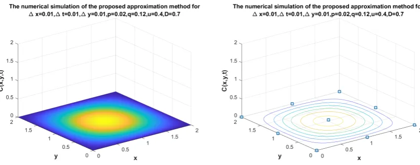
Figure 1. The numerical simulation of the proposed approximation method for equation (9) with ∆x=0.01,∆t=0.01,∆y=0.01,p=0.02,q=0.12,u=0.4,D=0.24

Figure 2. The numerical simulation of the proposed approximation method for equation (9) with ∆x=0.05,∆t=0.05,∆y=0.05,p=0.02,q=0.12,u=0.4,D=0.3

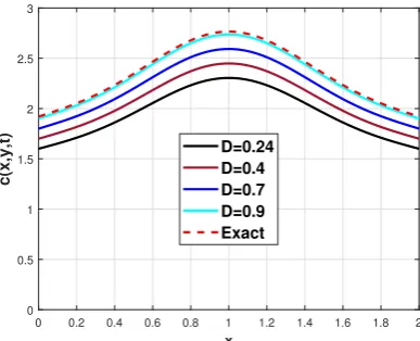
0 0.2 0.4 0.6 0.8 1 1.2 1.4 1.6 1.8 2

x

0 0.5 1 1.5 2 2.5 3

c(x,y,t)

D=0.24 D=0.4 D=0.7 D=0.9 Exact

Figure 4.The comparison of the obtained solutions of the proposed approximation method and exat solution for equation (9) with various values ofD.

Figure 5.Comparison between exact and approximate solution for equation (9) with various values of D.

0 10 20 30 40 50 60 70 80 90

t -0.1

-0.08 -0.06 -0.04 -0.02 0 0.02

Stability

D=0.5

0 10 20 30 40 50 60 70 80 90

t -1.2

-1 -0.8 -0.6 -0.4 -0.2 0 0.2 0.4

Stability

D=0.8

4. Numerical Investigation of the Present Study 141

In the present study, the unsteady convective-diffusion (in the both directions) partial differential

142

equation (9) together with the boundary (9a, b), entrance (9c, d) and initial (9e) conditions is solved

143

numerically by the finite difference scheme. For this, the first order derivative in time is approximated

144

by the second order difference formula and the diffusion terms in axial and radial directions is

145

expressed by the second order Crank-Nicolson difference operator. On one hand, the approximation of

146

convective term in the governing equation by central differences provides the non-physical oscillation

147

in the solution. On the other hand, upwind finite difference scheme gives the solution free from

148

the oscillation but it reduces the accuracy of the solution. Thus, for retaining the second order

149

accuracy of the solution for convective term, the Crank-Nicolson second order accuracy of the finite

150

difference scheme is used to approximate the convective term which provides the solution free from

151

the oscillations. The finite difference formulation leads to a system of linear algebraic equations which

152

needs a technique for computing the solution. It may be noted that the system has the tri-diagonal

153

character [34]. Such a system can be solved by the point iterative methods. However, the convergence

154

of the point iterative methods is very slow. In order to achieve faster convergence, we can use the line

155

iterative method. This method uses the tri-diagonal character of the coefficient matrix of equation, and

156

is easy to solve by the Thomas algorithm. Further, it may be noted that, by using this technique, the

157

equation involves an unknown c at every row for a fixed time level which saves the storage on the

158

computer. According to the Lax’s equivalence theorem, mathematical proofs of the numerical solution

159

technique were obtained. Hence, the consistency and stability of the equations were investigated which

160

assure the convergences. Computations have been done for ten intervals with x=0.1 in the positive

161

x direction, the step size y=0.1 in the positive y direction and the time step t=0.05 in the positive t

162

direction. The programs were tested even for the smaller step sizes. The technique described here can

163

be used to solve any linear system of unsteady convective-diffusion partial differential equation where

164

the axial diffusion term is ignored. Further, we may point out that the technique works in the equations

165

including axial diffusion term as well wherein we have done here in the form of the equation(9).

166

5. Numerical results 167

In this section, we show the numerical simulation of the proposed approximation method for

168

various values ofD,u,∆x,∆y,∆t,p,qto verify the efficiency of the proposed numerical method. The

169

numerical simulation of the proposed approximation method in Figures 1to 4are shown. The

170

behaviour of the obtained error for different values ofDare presented in Figure5. In Figure6stability

171

of the approximate solution for equation (9) with various values ofDare presented.

172

6. Conclusions 173

In the present study, we have considered a mathematical model for studying the non-steady

174

transport of oxygen in a slab of capillary. The capillary is assumed to be a two-dimensional channel

175

in dimensionless form. We have found that the difference equation which is described here, has the

176

same higher order of accuracy, wherein we want to achieve. We have increased the order of accuracy

177

from our previous studyO[(∆t) + (∆y) + (∆x)2][35], to the present higher order scheme using the

178

Crank–Nicolson method, i.e.,O[(∆t)2+ (∆x)2+ (∆y)2]. For stability condition, we have seen that, the

179

equations presented in the previous sections, are all stable and the results converges well. Further,

180

numerical results show that the axial diffusion does not effect the process of the oxygenation in a slab

181

of the capillary.

182

Acknowledgments 183

The authors wish to thank the unknown referees for their valuable comments and suggestions.

References 185

1. Wu, W.T.; Li, Y.; Aubry, N.; Massoudi, M.; Antaki, J.F. Numerical simulation of red blood cell-induced 186

platelet transport in saccular aneurysms.Appl. Sci.2017,7, 484. 187

2. Bridges, C.; Karra, S.; Rajagopal, K.R. On modelling the response of the synovial fluid: Unsteady flow of a 188

shear-thinning , chemically-reacting fluid mixture.Comput. Math. Appl.2010,60, 2333. 189

3. Hund, S.J.; Antaki, J.F. An extended convection diffusion model for red blood cell-enhanced transport of 190

thrombocytes and leukocytes.Phys. Med. Biol.2009,54, 6415. 191

4. Wu, W.T.; Massoudi, M. Heat transfer and dissipation effects in the flow of a drilling fluid.Fluids2016,1, 4. 192

5. Massoudi, M.; Antaki, J. An anisotropic constitutive equation for the stress tensor of blood based on mixture 193

theory.Math. Probl. Eng., doi:10.1155/2008/579172. 194

6. Skorczewski, T.; Erickson, L.C.; Fogelson, A.L. Platelet motion near a vessel wall or thrombus surface in 195

two-dimensional whole blood simulations.Biophysical J.2013,104, 1764. 196

7. Burger, J.M. Numerical study on non-linear Burger’s and modified Burger’s equations using B-Splines. 197

Internet Connection. 198

8. Zhan, W.; Wang, C.H. Convection enhanced delivery of chemotherapeutic drugs into brain tumour.J. Control. 199

Release2018,271, 74.

200

9. Kaesler, A.; Rosen, M.; Schmitz-Rode, T.; Steinseifer, U.; Arens, J. Computational modelling of oxygen 201

transfer in artificial lungs.Artif. Organs2018, doi:10.1111/aor.13146. 202

10. Melnik, R.V.N.; Jenkins, D.R. On computational control of flow in airblast atomisers for pulmonary drug 203

delivery.Int. J. Pharm.2002,239, 23. 204

11. Mountrakis, L.; Lorenz, E.; Hoekstra, A.G. Where do the platelets go? A simulation study of fully resolved 205

blood flow through aneurysmal vessels.Interface Focus2013, doi:10.1098/rsfs.2012.0089. 206

12. Whittle, I.R.; Dorsch, N.W.; Besser, M. Spontaneous thrombosis in giant intracranial aneurysms.J. Neurol. 207

Neurosurg. Psychiatry1982,45, 1040.

208

13. Hirabayashi, M.; Ohta, M.; Rüfenacht, D.A.; Chopard, B. Characterization of flow reduction properties in an 209

aneurysm due to a stent.Phys. Rev. E2003,68, 021918. 210

14. Weir, B. Unruptured intracranial aneurysms: A review.J. Neurosurg.2002,96, 3. 211

15. Desai, C.S.; Johnson, L.D. Evaluation of some numerical schemes for consolidation.Int. J. Numer. Methods 212

Eng.1973,7, 243.

213

16. Aminataei, A.; Sharan, M.; Singh, M.P. A numerical solution for the non-linear convective facilitated diffusion 214

reaction problem for the process of blood oxygenation in the lungs.J. Nat. Acad. Math.1985,3, 182. 215

17. Aminataei, A.; Sharan, M.; Singh, M.P. A numerical model for the process of gas exchange in the pulmonary 216

capillaries.Ind. J. Pure. Appl. Math.1987,18, 1040. 217

18. Aminataei, A.; Sharan, M.; Singh, M.P. Two layer model for the process of blood oxygenation in the 218

pulmonary capillaries-parabolic profiles in the core as well as in the plasma layer.Appl. Math. Modelling. 219

1988,12, 601.

220

19. Aminataei, A. A numerical two layer model for blood oxygenation in lungs.Amir-Kabir J. Sci. Tech.2001,12, 221

63. 222

20. A. Aminataei, Comparision of explicit and implicit approaches to numerical solution of uni-dimensional 223

equation of diffusion,J. of Sci., Al-Zahra Univ.2002,1, 15. 224

21. A. Aminataei, Blood oxygenation in the pulmonary circulation: a review,Euro. J. Scien. Res.2005,10, 55. 225

22. A. Aminataei, A numerical simulation of the unsteady convective-diffusion equation,The J. of Damghan Univ. 226

of Basic Scis.2008,1, 73.

227

23. A. Aminataei and S. Hassani, An efficient numerical method for the solution of initial and boundary values 228

problems,J. of Sci., Al-Zahra Univ.2009,22, 13. 229

24. E.F. Leonard and S.B. Jørgensen, The analysis of convection and diffusion in capillary beds,Annu. Rev. 230

Biophys. Bioeng.1974,3, 293.

231

25. A. Aminataei, Simulation of the breathing gases in the airways,J. Advan. Math. Model.2012,1, 51. 232

26. Aminataei, A. A mathematical model for oxygen dissociation curve in the blood.Eur. J. Sci. Res.2005,6, 5. 233

27. Lapidus, L.; Pinder, G.F.Numerical Solution of Partial Differential Equations in Science and Engineering; John 234

Wiley & Sons: New York, NY, USA, 1982. 235

29. Sharan, M.; Singh, M.P.; Aminataei, A. A numerical model for blood oxygenation in the pulmonary 237

capillaries-effect of pulmonary membrane resistance.BioSystems1987,20, 355. 238

30. Lax, P.D.; Richtmyer, R.D. Survey of the stability of linear finite difference equations.Commun. Pure Appl. 239

Math.1959,9, 267.

240

31. Evans, G.; Blackledge, J.; Yardleg, P.Numerical Methods for Partial Differential Equations; Springer-Verlag: 241

London, UK, 2000. 242

32. Smith, G.D.Numerical Solution of Partial Differential Equations: Finite Difference Methods; Oxford University 243

Press: Oxford, UK, 1993. 244

33. Noye, J.Numerical Simulation of Fluid Motion; North-Holland: Amsterdam, The Netherlands, 1978. 245

34. Thomas, L.H. Elliptic Problems in Linear Difference Equations Over a Network. Watson Scientific Computing 246

Laboratory, New York, Columbia University, 1949. 247

35. Aminataei, A. Numerical simulation of the process of oxygen mass transport in the human pulmonary 248