Unveiling the Hidden Rules of Spherical Viruses
using Point Arrays
David Wilson1
1 Department of Physics, Kalamazoo College, Kalamazoo, MI 49006, USA 1; [email protected]
* Correspondence: [email protected]; Tel.: 1-(269)-337-7096
Abstract: Since its introduction, the Triangulation number has been the most successful and ubiquitous scheme for classifying spherical viruses. However, despite its many successes, it fails to describe the relative angular orientations of proteins, as well as their radial mass distribution within the capsid. It also fails to provide any insight into critical sites of stability, modifications or possible mutations. We show how classifying spherical viruses using icosahedral point arrays, introduced by Keef and Twarock, unveils new geometric rules and constraints for understanding virus stability and key locations for exterior and interior modifications. We present a modified fitness measure which classifies viruses in an unambiguous and rigorous manner, irrespective of local surface chemistry, steric hinderance, solvent accessibility or triangulation number. We then utilize these point arrays to explain the immutable surface loops of bacteriophage MS2, the relative reactivity of surface lysines in CPMV and the non-quasiequivalent flexibility of the HBV dimers. We explain how using sister and double point arrays can function as predictive tools for site directed modifications in other systems. This success builds on our previous work showing that viruses place their protruding features along the great circles of the asymmetric unit, demonstrating that viruses indeed adhere to these geometric constraints.
Keywords: protruding features; spherical virus; point arrays; surface modifications; VLP; drug delivery; icosahedral; nanomedicine; ligand binding
1. Introduction
We present a modified fitting method for classifying spherical viruses using the 55 single and 513 double icosahedral point arrays which were introduced by Keef and Twarock [1]. We offer new interpretations of these point arrays as geometric restrictions that place constraints on which amino acids are possible to modify. We also discuss how these point arrays might be utilized to determine new potential locations for significant external or internal capsid modifications such as decoration proteins or ligand binding.
Spherical viruses have been canonically well described by their Triangulation number (T-number), introduced by Caspar and Klug [2], which posits that capsid proteins are arranged in such a manner as to have nearly identical chemical environments, known as quasi-equivalence. In general, the T-number specifies the total number of proteins needed(60T)to form the capsid, as well as the number of proteins within the asymmetric unit(T)(Figure1) and that there are 12 pentamers and 10(T−1) hexamers subunits in a capsid. While there are several notable exceptions to these rules, each of these exceptions is arranged in the same subunit layout as the canonical T-numbers. For example L-A virus, is a 120 protein capsid (T=2) with the same architecture as a T=1 capsid, though it has 10 proteins making up its pentameric unit and no hexamers. Also of note is SV40, which has a T=7d architecture. SV40 is composed entirely of pentameric subunits, with 60 pentamers residing where the 60 hexamers would normally be located, reducing the capsid from 420 proteins to 360 proteins. The T-number is also able to describe capsids with pseudo-Triangulation (pT) numbers, which are composed of multi-domain proteins which form pseudo-pentamers and pseudo-hexamers to resemble a larger T-number capsid. CPMV is an example of a pT3, which has the same subunit architecture as a
T=3 capsid, appearing to be composed of 12 pentamers and 20 hexamers, though only containing 60 proteins instead of 180 proteins. While theT-number is a powerful description, it is fundamentally a limited tool as it uses a 2dthin-shell description, that only specifies the general protein arrangement of the viral capsid, and does not specify where or how capsid proteins are oriented, nor their radial distribution nor any information about the organization of the genetic material contained within.
It has been demonstrated that several spherical viruses conform to the geometric constraints of the icosahedral point arrays introduced by Keef and Twarock et al. [1,3]. The points of these arrays represent material boundaries at multiple radial levels for proteins, genetic material and their interfaces. Each point array imposes a different set of radial and angular constraints on the virus [1,3,4]. The geometry of viral architecture has also been explored by Janner [5–9] using encasing forms which are constructed for viral components at different radial levels by embedding virus structure into lattices. Janner has also explored fitting point arrays by hand to viral capsids, and has argued that a more specific toolkit should be developed for the analysis of the viral architecture, including comparisons with indexed backbone positions and regions with site specific point symmetry [10]. We showed using these 55 point arrays, that viruses place their protruding features at discrete gauge points along the 15 icosahedral great circles of the asymmetric unit (Figure1), a direct consequence of viruses conforming to these geometric constraints [4]. These gauge points refer to the overall scaling of the point array. Another promising method of icosahedral point array generation has been offered by Zappa et al. [11,12], who propose generating point arrays from 6d projections of the hypercube. The fitting methods in this paper are compatible with this scheme, if a systematic library can be developed. Point arrays are a natural tool for measuring and characterizing spherical capsids, as they can be used to track changes throughout maturation as well as to quantify individual structural feature differences between capsids. In recent years, additional capsid descriptions have been offered, including an expanded Triangulation number by Rochal et al. [13] and icosahedral surface tiling by Twarock et al. [14], though each of these schemes focuses on surface organization rather than a detailed radial description.
In this work we will present an improved fitness algorithm which utilizes the gauge point fitting of protruding features to determine the best fit to the point arrays developed by Keef and Twarock [1] to characterize the viral architecture of spherical viruses. This improved algorithm was needed to clarify and remove poorly matching point arrays that were found to fit viruses in Refs [3,15]. Through gauge point filtering and removal of several free parameters, we have greatly clarified the fits of these point arrays. We will also show how to utilize these point array fits to suggest surface sites where virus capsids should and should not be modified, independent of their local chemistry, including the relative reactivity of surface Lysine residues of the pseudo T=3 (pT3) CPMV [16,17]. We will demonstrate that the location of protruding features can dramatically limit the possible interior structure of viruses, including the placement of interior drug placements for potential therapeutic VLPs.
2. Materials and Methods
maximum relative distance and orientation of the capsid protein features. In some cases these limits will also impose constraints on packing of the genetic material contained within.
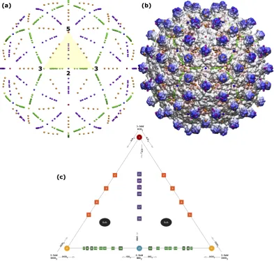
Figure 1.(a)The spatial distribution of gauge points have icosahedral symmetry,i.ethey have 2-, 3- and 5-fold symmetry axes as shown. There are 15 icosahedral great circles which connect nearest neighbor symmetry axes. We refer to these sections of the circles subtending 5, 2 and two 3 fold axes shown as the 5-2 GC, 5-3 GC and the 2-3 GC. The volume bounded between these circles in known as the asymmetric unit (yellow). The asymmetric unit (AU) is a representative one sixtieth section of the entire capsid (yellow). The gauge points all lay on these icosahedral great circles [4] and are colored as in Table1.(b)The gauge points have been placed on a radially colored HBV (1qgt) capsid at their small possible distance from the protein surface. We will later see that the only admissible gauge points are the purple and orange elements sitting atop the protruding dimers.(c)There are 21 unique gauge points in the asymmetric unit, see Table2. The gauge points on the 2-,3- and 5-fold axes only result fromαIDD2,
αDOD3andαICO5point arrays, respectively, whereαis the scaling length. The remaining gauge points on the great
circles come from exactly two different sister point arrays,e.g.Gauge Point 4 (GP:4) is created only fromφ0ICO3
andφDOD5. In total of 36 of the 55 point arrays have gauge points which are not located on the symmetry axes.
Points not on these great circles are referred to as bulk points.
2.1. Icosahedral Symmetry
Figure 2. A structural comparison showing the wide diversity in viral capsid shapes of even the simplest T=1 viruses. Each virus capsid has been radially colored, with red being the most interior, and blue the exterior. These three,(a)Infectious Bursal Virus (Avibirnavirus, 2gsy) [18],(b)Hepatitis E Virus Like Particle (Hepevirus, 3hag) [19], and(c)Penton Base of Adenovirus A (Mastadenovirus, 4aqq) [20], were chosen as they have almost no overlap in their protruding features. The best fit point array for each capsid is listed, as we will see, these point arrays describe unique features and complement the T-number classification. The asymmetric unit of each capsid is contained by the triangular region of gauge points (Figure1).
rotation matrices can be generated by successive combinations of the 2-fold rotationaand the 3-fold rotationbwhich border the asymmetric unit (Figure1), as
I ≡Da,b|a2=b3= (ab)5=1E. (1) The rotation matrices and all of our polyhedral vertices appear in the Appendix.
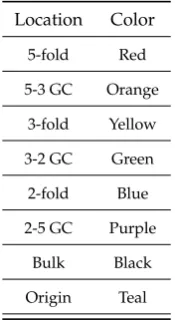
Table 1. The color scheme used for point array elements throughout this paper. Each color specifies the type of geometric location,e.g.5-fold axes are red, 2-fold axes are blue, and purple are the points on the great circle between the two (Figure1).
Location Color
5-fold Red
5-3 GC Orange
3-fold Yellow
3-2 GC Green
2-fold Blue
2-5 GC Purple
Bulk Black
Origin Teal
We begin with the vertices of the three standard (base) representations of icosahedral symmetry the icosahedron, dodecahedron and icosadodecahedon (Figure 3) which are representations of the 5, 3 and 2-fold symmetries respectively. The vertices of these polyhedra will also serve as our translation vectors for the affine extensions below. We align all of our structures with the Viper Database orientation [21] of the spherical volume with a 2-fold axis aligned with the +z direction and a 5-fold aligned with the vector(0, 1,φ), whereφ= 1+
√
5
2 ≈1.618 is the golden ratio . The
vertices of each of the three respective polyhedra are all equidistant from the origin and therefore constitute only a single radial level.
Throughout this work we will show images of point arrays layered atop virus capsids. We have introduce a standard color scheme, inspired by the icosahedral building kits made by Zometool. The symmetry axes have primary colors 5-fold (red), 3-fold (yellow) and 2-fold (blue). The points along the great circles connecting neighboring symmetry axes (Figure1) are based on the paint color addition of those two colors, see Table1.
2.2. Affine Extensions
Figure 3.The three standard polyhedrons with icosahedral symmetry and the affine extension translation vectors.
(a)The 12 vertices of the icosahedron are on the six 5-fold axes and the structure is generated by applying all 60 icosahedral rotations on a single point[0, 1,φ], which also serves as the translation vector~T5.(b)The 20 vertices of
the dodecahedron are on the ten 3-fold axes and the structure is generated by applying the full icosahedral group to the point[−φ0, 0,φ], which also serves as the~T3translation vector.(c)The 30 vertices of the icosadodecahedron
are on the fifteen 2-fold axes and the structure is generated by applying the full icosahedral group to the point
1
2[−1,φ2,φ], which serves as the~T2translation vector.
in the intersection of two or more vertices of the base polyhedron (ICO, DOD or IDD) [3]. This intersection reduces the cardinality (number of elements) of the point array from the maximal free group representation and is required to be admissible. The construction begins by translating ICO, DOD or IDD in the 2-fold(~T2), 3-fold(~T3)or 5-fold(~T5)direction, scaled by a translation amount λ. This translation is referred to as an affine extension. As this translated set of points no longer has
icosahedral symmetry at each radial level, we restore the symmetry by applying the 60 icosahedral rotations to form the complete point array (Figure4). The point arrays can be considered to have two components, the base vertices and the point cloud generated by applying icosahedral symmetry to the affine extension. Affine extensions are linear transformations which preserve parallel relationships within a geometric representation, however they do not preserve local angles or distances and are a standard tool for extending group symmetry.
For example we could determine which scaling length(s)(λ)for the translationλ~T5would result
in an intersection. One of the solutions isλ= φ1, which causes three vertices of ICO to intersect at a
3-fold axes, thus reducing the cardinality. This process is illustrated in Figure4. We represent this point array as ICO∪ I(ICO+φ~T5), which is the union (∪, combination) of the base polyhedron ICO
and the point cloud generated by the 60 icosahedral rotationsI of the translated vertices ICO+φ~T5.
This approach might seem ill-conceived, as icosahedral symmetry is the largest compact rotation symmetry in 3d. However, this method does add any new symmetry axes, rather it creates a representation of icosahedral symmetry at multiple radial levels. These representations have specified ratios of radial levels with only one free parameters, overall scaling of the point array. It has been suggested that this extended symmetry could help explain the inherent stability of viral capsids [3].
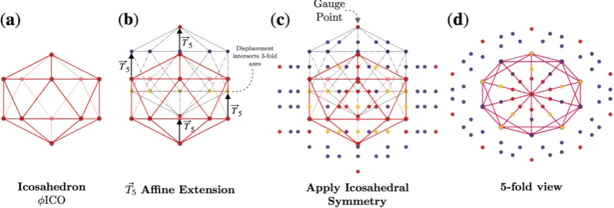
Figure 4.Formation of theφICO5point array [1].(a)The base of this point array is an icosahedron scaled up by
multiplying byφ.(b)The base point array is then translated by~T5. Under this~T5extension, the base point array
consists of 4 separate levels. The lowest level is a single vertex which remains on the 5-fold axes, the next level of 5 vertices all intersect 3-fold axes (all with the same radius). The next level ends up on the 5-2 great circle of the AU, resulting in 60 points, finally the gauge point of the point array is created by the largest radius point (Figure5).(c)
Icosahedral symmetry is now applied, creating the full point array (base and cloud), the points are colored as in Figure1. As the translation was~T5, the resulting gauge point remains on the 5-fold axes (Figure1)(d)A look down
one of the twelve 5-fold axes shows the the point array has icosahedral symmetry. This entire point is enveloped by a now larger icosahedron, with the purple points sitting on its edges. The formation of point arrays can equivalently be described as placing an icosahedron centered at each of the original base vertices to create the point cloud.
Figure 5. A histogram of the radii of the point array elements in arbitrary units. The base arrayφICO has a
bold outline around the 12 points atr∼0.64. The gauge point is on the 5-fold axes (Gauge Point 1). In total there are now 3 icosahedrons and one dodecahedron, all with different radii. There is also a layer of 60 points along the 5-2 great circle of the AU; due to the 60 rotations of the icosahedral group, any point not on a symmetry axes will yield 60 points after the symmetry is applied (Figure4). The cardinality or size of this point array is 116=12(ICO) +20(DOD) +12(ICO) +60(5-2) +12(ICO).
For ease of notation and formation of double point arrays, we rescale each of the base polyhedra so that their translation lengths,λ = 1, for each of the respective translation vectors,T2,T3orT5.
This rescaling leaves the point arrays equivalent up to an overall scaling and does not affect any aspect of their applications to virology. All scaling lengths can be written in the form 2mφn, where
m,n = −3, . . . , 3, whereφ= 1+
√
5
ICO
|{z} base
∪ I(ICO+
Affine Extension z}|{
φT5 )
| {z }
point cloud
→φ0ICO∪ I φ0ICO+T5
≡φICO5
Two or more point arrays with the same affine extension vector may be combined to form a larger point array,e.g.φICO5and DOD5may be combined asφICO5∪DOD5, as seen in Figure6. One way
to think of this union is that instead of staring with the baseφICO, you begin with the combined
baseφICO∪DOD and then translate this double base by~T5 and re-apply icosahedral symmetry.
Forming larger point arrays can be desirable for several reasons, including searching for additional constraints on the virus architecture or to find compatible internal or external structural modifications sites. We consider the set of 55 single base point arrays and 513 double base point arrays for our fitness measure.interpretation is that there are two base point arrays which are extended .
Figure 6.Formation of a Double Base Point Array. Here(a)point arrayφICO5and(b)point arrayφDOD5have
the same affine extension~T5and may therefore be combined to form(c)(ICO∪DOD)5a double base point array.
(d)A view down a 5-fold axes after applying icosahedral symmetry, the points originating fromφDOD5are shown
Comparing Different Options of Point Array Combinations
Figure 7.Here we examine two ways to form double point arrays withφICO5. As before, the base polyhedra are
outlined in bold. In(a)we examine the formation of ofφICO5∪φDOD5which adds points above the icosahedral
envelopment ofφICO5and could be used to locate a site for surface modification of the capsid. The cardinality of
φICO5andφDOD5is 116 and 172 respectively (Table2), however each of these point arrays respectively generate
the base of the other array, reducing the cardinality from 288 points to 256 points, with 8 radial levels, rather than 10. We also see the formation of(b)φICO5∪2IDD5which adds surface points near the same radial level as the original
gauge points ofφICO5. The cardinality of 2IDD5is 242 and none of the points overlapφICO5, therefore the total
2.3. Major Features of Point Arrays
At first glance, the library of point arrays appears to have a large number of degrees of freedom, which might seem to accommodate any architecture, however the constraints implied by each point array are quite specific, and the restriction of outer features of the viral capsid being coincident with gauge points considerably lowers the freedom of building spherical viruses. An important feature of each of these point arrays is that icosahedral symmetry now occurs on several radial levels (Figure5) and (Figure7). Each point array has only one free parameter, the overall radial scaling. Every other aspect is fixed, including the radial distribution, relative angular positions and positions of the points. The major features of the point arrays are
1. 55 Unique Single Point Arrays- there are 13 point arrays formed from~T5 = [0, 1,φ], 17 point
arrays formed from~T3= [1/φ, 0,φ]and 25 point arrays formed from~T2 = [0, 0,φ]extensions.
Forty one of these point arrays have points on the icosahedral symmetry axes at 2 or more radii. The remaining 14, which are only formed from the DOD and IDD bases withT2orT3extensions,
have only one radial level with points on the icosahedral symmetry axes. It is worth noting that in all of the affine extensions, no non-icosahedral symmetry appears nor do any new accidental icosahedral axes. This is due to the fact that the icosahedral group is the largest discrete compact rotation group in 3 dimensions. Generally, point arrays involving IDD or~T2extensions have the
most number of points.
2. Gauge Points- The set of outermost points from all of the 55 point arrays reveal there are only 21 unique locations within the AU, known as gauge points because they determine the scaling of the entire point array (Figure1). These points are required to be in agreement with protruding features [4]. This limited set of locations has important implications connecting the protrusions of viruses to their internal structure. Once the gauge points are know, there is an absolute maximum distance between the gauge point and next radial level which can not be transformed or scaled away, and this next radial level must coincide with the capsid proteins or the entire point array must be discarded. This implies new rules for modifying external and interiors surfaces of virus capsids. Protruding features located on these gauge points are referred to as Wilson Protrusions. The reason there are only 21 locations is that multiple point arrays generate the same gauge points,e.gφ0ICO3andφDOD5begin as different polyhedra, but after translation, arrive at the
same gauge point, see Table2. The 18 gauge points which are not on symmetry axes come from exactly two point arrays, referred to assister point arrays.
3. Sister Point Arrays - Most of the single base 55 point arrays have a nearly identical sister array. These point arrays have identical point clouds up to an overall radial scaling, see Table2. An example of these point arrays isφICO2 = φICO∪ I(φICO+T2) andφ0IDD5 =
1
φIDD∪ I
1
φIDD+T5
. Each point array has GP:21 and they have identical point clouds (Figure8). The only difference is their base point array and the point arrays which they can be combined. We believe that if one knew the location of the genetic material of a virus, they could distinguish between these two point arrays. We write sister point arrays with a tilde∼, e.g.φICO2∼φ0IDD5. In total there are 26 of the point arrays which only differ at a single radial
level, their base polyhedron and otherwise have identical point clouds. This brings the effective number of distinct point clouds down to 29. We also notice that there are six enveloping shapes for these point arrays ICO3∼DOD3, ICO2∼IDD5, DOD2∼IDD3, ICO5, DOD3and IDD2.
4. Double Base Point Arrays- There are 5131unique possible combinations of 2 single base point arrays resulting from the pairing of the 55 starting configurations with the same translation vector [1,3,15], (Figure6and7). In this work, we only consider the 568 single and double base point
1 Two of the possible pairings result in identical point arrays resulting in only 513 combinations rather than 514 originally
arrays. We write the largest relative radius point cloud first. We will see that double point arrays can improve fit and/or suggest sites for modification in the results for the Hepatitis E VLP. In general, double point arrays do not have sister double point arrays, as the translation vectors change. When double point arrays do have sister point arrays which can still be combined, the radial ordering of these point arrays reverses, creating a very different structure than the original double array. For example, 2φ0IDD5∪IDD5 has as its combined sisters point array ,
ICO2∪0.5φICO2, which swaps the top and bottom point arrays. Double point arrays can be
formed by pairing any of the two point arrays in theT5,T3orT2list, see Table2.
5. Single Free Parameter- While there can be many point arrays to consider, it is important to stress that each point array only has a single free parameter, the overall radial scale. We are not free to eliminate points that we do not like, although we do disregard layers of points below the viral capsid when matching point arrays to capsids, unless the genetic material is known (see fitness procedure in the next section).
Comparison of Two Sets of Sister Point Arrays
Figure 8.The radial distribution of point clouds for sister point arrays are identical, except for the base arrays (shown in bold outline). In(a)φ0ICO3is identical toφDOD5except for their two basesφ0ICO andφDOD. Note that
these point arrays have different affine extensions, so they can not be combined. In(b)IDD5is identical to ICO2
except for IDD and ICO. The bulk points atr∼.75 have two sets of 60 points one on the left and right side of the 5-2 great circle in the AU. While these points have the same radius, they are not equivalent locations.
2.4. Radially Ordered Single Base Point Arrays
Here we present a new radial ordering of the 55 single point arrays and their sister point arrays in Table2. The point arrays have been ordered from largest to smallest relative radius, to aid in the construction of similar radial size double point arrays. For example, consider a virus fit byφDOD5
and you want to find locations potentially favorable to surface modification, start by examining 2IDD5
which provides new geometric constraints which are above those inφDOD5. These 55 point arrays
The 13 T5Affine Extensions
Scale Base GP Loc Lvs Size Sister(∼) 2φ IDD5 16 5-2 6 290 .5φ0 ICO2 φ2 DOD5 5 5-3 5 200 φ02 ICO3
φ ICO5 1 ~5 5 116 φ0 ICO5
2 IDD5 17 5-2 6 242 0.5 ICO3
φ DOD5 4 5-3 5 172 φ0 ICO3
1 ICO5 1 ~5 5 85 − −
2φ0 IDD5 18 5-2 6 242 .5φ ICO3
1 DOD5 3 5-3 5 172 1 ICO3
1 IDD5 19 5-2 7 360 1 ICO3
φ0 ICO5 1 ~5 5 116 φ ICO3
2φ02 IDD5 20 5-2 6 290 .5φ2 ICO3
φ0 DOD5 2 5-3 5 200 φ ICO3
φ0 IDD5 21 5-2 7 360 φ ICO3 The 17 T3Affine Extensions
Scale Base GP Loc Lvs Size Sister(∼) 2φ IDD∗3 14 2-3 9 510 .5φ0 DOD∗2 φ2 DOD∗3 6 3-fold 8 360 φ02 DOD∗3 2 IDD3 13 2-3 8 362 .5φ0 DOD2
φ ICO3 2 5-3 5 192 φ0 DOD5
φ DOD3 6 ~3 7 252 φ0 DOD3
2φ0 IDD3 12 2-3 9 374 .5φ DOD2
1 DOD3 6 ~3 7 191 − −
1 ICO3 3 5-2 5 164 1 DOD5
1 IDD3 11 2-3 11 600 1 DOD2
2φ02 IDD3 10 2-3 8 362 .5φ2 DOD2
φ0 DOD3 6 ~3 7 252 φ DOD3
φ0 ICO3 4 5-3 5 164 φ DOD5
φ0 IDD∗3 9 2-3 10 570 φ DOD∗2 2φ03 IDD∗3 8 2-3 9 510 .5φ3 DOD∗2 φ02 DOD∗3 6 ~3 8 360 φ2 DOD∗3
φ02 ICO3 5 5-3 5 192 φ2 DOD5
φ02 IDD3 7 2-3 11 600 φ2 DOD2
The 25 T2Affine Extensions
Scale Base GP Loc Lvs Size Sister(∼) 2φ IDD∗2 15 2-fold 16 870 .5φ0 IDD∗2 φ2 DOD2 7 2-3 11 590 φ02 IDD3 φ2 IDD2 15 2-fold 14 710 φ02 IDD2 .5φ3 DOD∗2 8 2-3 9 500 2φ03 IDD∗3 2 IDD∗2 15 2-fold 16 870 .5 IDD∗2 φ ICO2 21 5-2 7 342 φ0 IDD5 φ DOD∗2 9 2-3 10 560 φ0 IDD∗3 φ IDD2 15 2-fold 12 552 φ0 IDD2 .5φ2 ICO2 20 5-2 6 272 2φ02 IDD5 .5φ2 DOD2 10 2-3 7 332 2φ02 IDD3 2φ0 IDD2 15 2-fold 16 870 .5φ IDD2
1 ICO2 19 5-2 7 342 1 IDD5
1 DOD2 11 2-3 11 590 1 IDD3 1 IDD∗2 15 2-fold 9 361 − −
.5φ ICO2 18 5-2 5 212 2φ0 IDD5 .5φ DOD2 12 2-3 8 344 2φ0 IDD3 .5φ IDD∗2 15 2-fold 16 870 2φ0 IDD∗2 φ0 IDD2 15 2-fold 12 552 φ IDD2 0.5 ICO2 17 5-2 5 212 2 IDD5
0.5 DOD2 13 2-3 7 332 2 IDD3
0.5 IDD∗2 15 2-fold 15 840 2 IDD∗2 φ02 IDD2 15 2-fold 14 710 φ2 IDD2 .5φ0 ICO2 16 5-2 6 272 2φ IDD5 .5φ0 DOD∗2 14 2-3 9 500 2φ IDD∗3 .5φ0 IDD∗2 15 2-fold 16 870 2φ IDD∗2
Table 2.The 55 Admissible Point Arrays [1,3], grouped by extension vectorsT5,T3orT2, ordered from largest
2.5. Point Array Fitness Algorithm
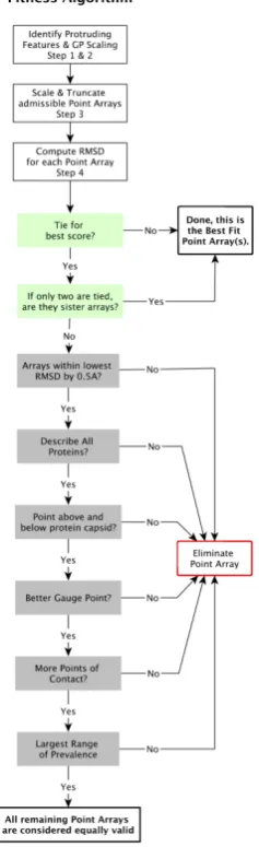
We now present our modified point array fitness algorithm which includes gauge point agreement, low relative surface RMSD and characterization of all capsid proteins (Figure 9).
Figure 9.Schematics representation of the fitness algorithm for point array matching to viral capsids. Most viruses only have a few point arrays that have a low RMSD. Many ties are due to sister point arrays.
1. Identify Protruding Features of a Virus- Our algorithm determines the most radially distal protruding features of each viral capsid. As these external features can be critically important in the lifecycle of the virus, and we previously showed nearly all spherical viruses use the set of gauge points for their protrusions, we prioritize their placement. In practice, we have found that the outer 3% of atoms by radius in a capsid are sufficient for finding protruding features. We then cluster all atoms in the outer 3% with those below them in the upper half of the capsid. We consider this as our protrusion and find its geometric center of mass, treating all atoms as if they have the same mass. This process is described in more detail in our previous work on protruding features [4].
2. Determine Gauge Point Scaling- We begin all of the 21 gauge points 5 angstroms beyond the atom with the largest radius. We then allow them to fall radially onto the capsid. A gauge point is stopped when it reaches its nearest distance to the protein surface, which we model as an overlap of 1.5Å spheres which is slightly smaller than the average van der Waals radii of each of the heavy atoms [22]. If a gauge point would fall through the surface of the capsid, we stop it at its point of closest approach. We only consider point arrays with gauge points located on or near these protruding features, referred to as admissible gauge points [4]. This dramatically reduces the number of point arrays which need to be considered when characterizing viruses, see Table2. The gauge points are presented in Figure1. An example of this step applied to Hepatitis B can be seen in Figure10& (b). The yellow gauge points on the 3-fold axis would have fallen through the capsid, but were stopped at the location of nearest approach. The determination of the admissible gauge points will prove to be a critical step in understanding the restrictions conferred by point array geometries on the entire capsid structure.
3. Scale and Truncate Point Arrays- We now scale point arrays with admissible gauge points to match the virus capsids. Generally point arrays cover a larger radial extent than the capsid proteins, going well into the interior of the virus. We interpret
4. Compute RMSD from Truncated Point Arrays to the Viral Capsid Proteins- We now compute the surface RMSD [3] for the point array elements within the asymmetric unit according to
Rsurf=
N
∑
i=1
mipid2i N
∑
i=1
mipi
1/2
(2)
wherediis the minimum distance from theithpoint array element to the nearest protein surface(s),
piis the protein multiplicity (number of distinct proteins) near the pointi(e.g.5 for a point on a
5-fold axes, or 2 if two proteins are equidistant from the same point. Finallymiis the number of
times the point appears in the full point array (e.g.,12, 20, 30 etc) andNis the total number of point array elements. Protein multiplicity is a weighting factor for when two or more proteins are roughly equidistant from a point to within a few tenths of an angstrom, it has a larger weight piin the RMSD,e.g., if a point array element were sitting on a 3-fold axis, it would be counted 3
times. Figure10provides an example of multiplicitypiand the number of times a point appears
in the AU of the point arraymi.
We minimize the RMSD by radially shunting the entire point array radially by±5 Å in 0.25 Å steps. During this shunting, we eliminate point arrays which contain points within the protein surfaces or small pockets, as point arrays represent external material boundaries [3,15]. We do not allow further interior point array elements to be cutoff during this optimization, we refer to this as gauge fixing. This modified algorithm eliminates most spurious point arrays from considerations, improving upon the fits of [3].
5. Determine Best Fit Point ArraysIn general, we only find a handful of point arrays which have the correct gauge point(s) and low RMSD. Often a point array and its sister point array will both meet the same criteria and without knowledge of the genetic material, they are indistinguishable. The following criteria to break ties
(a) If a point array has a lower RMSD score by 0.5 Å or more. (b) Have at least one element near each protein.
(c) Encase the protein capsid with points above and below.
(d) Have a better agreement with the gauge point fits, as seen in Figure11.
(e) Have more points of contact with capsid proteins,e.geach point on the five fold axes have at least 5 points of contact with protein surfaces. We consider this step after checking gauge point fits (d), as the number of contacts can be quite large for point arrays with IDD bases or~T2extensions which can considerably lower the RMSD score.
(f) Have the largest range of prevalence (Figure 10), indicating a wide range of radial agreement [3].
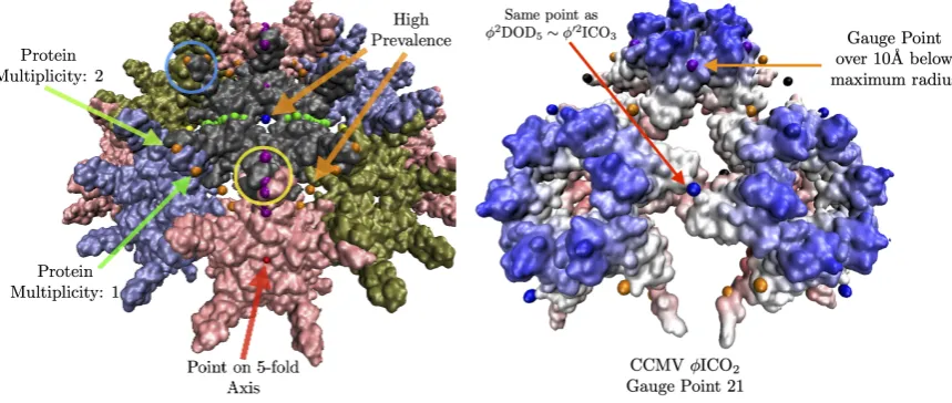
Figure 10. Features of the point array fitting algorithm. Here we have docked the gauge points on HBV, a T=4 virus with dimeric protrusions. We only consider the gauge points nearest the most radially distal protruding features,e.g., the nearest gauge points to the protruding dimers are GP: 17, 18 and 19 (yellow circles) and 4 and 5 (blue circles). Next we only consider the point arrays which contain these gauge points, see Table2. In this example, there are 3 gauge points that would have fallen through the capsid surface when docked, they were instead stopped at the distance of closest approach. Here we see most points sit on the surface of the proteins, and some on the symmetry axes in between proteins. Points that are near more than one protein are weighted more in the RMSD, through protein multiplicity pi, see Eq.2. High multiplicity always occurs at symmetry axese.g. gauge point 1 (red) on the 5-fold axis would count 5 times. There are several points which would lead to a high prevalencei.e. that is they do not intersect proteins over a large range of radial scaling, including gauge point 15 (blue) which is on a 2-fold axis and gauge point 3 (orange). In this example, these points would lead to a poor RMSD fit, as they are each several angstroms away from the surface.
Figure 11.A section of the swollen CCMV capsid radially colored and fit withφICO2. In our fitness
2.6. Comparison with Previous Measure
We will now review the key differences between Keef et al. [3] fitness measure and our own measure.
1. Gauge Point Agreement- We only allow point arrays with gauge points near the protruding features of viruses, dramatically limiting the number of point arrays to consider. This criteria is based on angular proximity with the protruding features, rather than overall scale of the point arrays, which has provided the single largest improvement to the fitness criteria.
2. Simplified RMSD Measure- The prior fitness measure used a topological RMSD in addition
to the surface RMSD, as RMSD=RMSD2surf+RMSD2top 1/2
, which was very sensitive to the overall radial scaling of the point arrays, and often had poor RMSDtopscores which could be
overcome by an abundance of good points, due to the large number of points offered by IDD and~T2systems, along the interior surfaces of the capsids. By contrast, gauge point agreement is
independent of radial scaling.
3. Gauge Fixing of Truncated Point Arrays- We make a single interior point array cutoff when the initial gauge point scaling is determined, which prevents poor interior points from being accidentally removed while optimizing the RMSDsurfscore.
4. Recognition of Sister Point Arrays- Many point array fits appear distinct, but upon inspection are doubly represented at the level of single base point arrays due to the radial truncation of the point arrays.
5. Tie Breaking Criteria- We introduce several criteria to break any RMSD ties, such as requiring at least one point per protein (Figure9). We also added a new criteria, that all point arrays have at least one point which corresponds to each protein within the asymmetric unit (AU). While we consider prevalence, we generally find that excluding point arrays due to their being located within a small pocket of a protein to be sufficient.
3. Results & Discussion
The locations specified by points arrays can serve as contact points for proteins, as well as external and internal material boundaries. The majority of the elements in these point arrays are located on the icosahedral great circles, for examples of these distributions see Figures5,7&8. We interpret these locations as boundary constraints in the sense of Janner’s encasing forms [5–9], for the protein capsid and genetic material contained within.
On one hand, this makes sense, as proteins can not be located directly atop the symmetry axes, so these points provide a convenient location for the proteins to maintain contact while adhering to the overall symmetry. We believe that some of these points might act as mechanical equilibrium locations for the icosahedral vibrational modes of the capsids. Given that the points are often sites of multiple protein contacts and that meeting these geometric restrictions appears to be advantageous, it is plausible that the proteins could be oscillating around these locations similar to a mass on a spring. We will see below that the chemically identical protein dimers of HBV have different vibrational properties which are consistent with the locations of the point array elements.
succeed, although not what form they should take. We will see that in MS2, the gauge points reveal critical structural locations which are nearly impossible to modify [23,24].
It can often be frustratingly difficult to modify protein capsids at particular locations, and the exact reasons are often unclear. Often sites appear ideal, based on local chemistry, solvent accessibility and a lack of steric hinderance. As we will see, knowledge of point array fits provides suggested sites to modify on the protein capsid, as well as sites that should not be modified, based on purely geometric constraints that would be overlooked in other analysis. A virus capsid’s adherence to the geometric constraints of point arrays likely stabilizes the protein capsid. It is also possible that these point arrays could specify multiple sites which must be modified in order to remain stable, depending on the distribution of point arrays by radius and the rules of combining point arrays.
3.1. Virus Point Array Classification
Here we present our results of the Point Array Fitness Algorithm for 16 viruses ranging over T = 1, 3, 4 and 7 virus capsids of RNA and DNA viruses in Table3. Overall we found that all viruses had only a single best array, up to sister fits, with RMSD values generally less than 2Å. The criteria that made the largest difference after RMSD ties were descriptions of all proteins, best gauge points and points above and below the capsid. We found that the only fits which could not be distinguished from other point arrays were the result of sister point arrays. Without knowing the locations of the genetic information, it is not possible in most cases to break this tie. Some notable exceptions are seen with Infectious Bursal Virus, Hepatitis E VLP and the Penton Base of Adenovirus A (Ad3), all T=1 viruses (Figure2). We will look at two of these viruses in more depth below.
Best Fit Point Arrays with RMSD Values
Name T PA RMSD (Å) GP NAU PDBID
Infectious Bursal Virus 1 .5φ3DOD2 4.5 8 9 2gsy, [18]
Hepatitis E VLP 1 2φIDD2∪φ2IDD2 2.8 15 26 3hag, [19]
Adenovirus Ad3 Dodecahedron 1 IDD5 3.7 19 7 4aqq, [20]
STMV 1 ICO3∼DOD5 1.2 3 3 1a34, [25]
L-A Virus 2 φDOD5∪DOD5 1.4 4 3 1m1c, [26]
Bacteriophage GA 3 φICO3∼φ0DOD5 0.2 2 2 1gav, [27]
Bacteriophage MS2 3 φICO3∼φ0DOD5 0.7 2 2 2ms2, [28]
CCMV Native 3 φ02ICO3 0.7 5 3 1cwp, [29]
CCMV Swollen 3 φ2DOD5 2.7 5 4 (a) [30]
Tobacco Necrosis Virus 3 φ0ICO5∪2φ02IDD5 0.9 1 5 1c8n, [31] Cowpea Mosaic Virus (CPMV) pT3 φ0ICO5∪2φ02IDD5 1.5 1 5 1ny7, [32]
Helicoverpa (HASV) 4 IDD5∪φ0ICO5 1.1 19 6 3s6p, [33]
Hepatitis B 4 ICO2∪.5ICO2 1.3 19 5 1qgt, [34]
Nudaurelia CapensisωVirus 4 DOD5∪φ0ICO5 1.5 3 5 1ohf, [35]
Bacteriophage P22 Mature 7l φICO5∪φDOD5 0.8 1 3 5uu5, [36]
HK97 Prohead II 7l φ0ICO5∪φ0IDD5 1.8 1 4 3e8k, [37]
Table 3.Here we present the results of our fitness algorithm of 16 viruses, considering RMSD scores, gauge points (GP), and points of contact (NAU). All fits are decided as in Figure9. Most RMSD fits are at least better than 0.5 Å than the next best array. Several viruses are equally well fit by a point array and its sister array. When both sister point arrays are equally valid,e.g.ICO3or DOD5of STMV, both are listed. If two point arrays are tied for best, that
is stated explicitly. All structures analyzed in this paper were taken from the Viper Database [21]. (a) There are two cryo-EM fit solutions for CCMV in the swollen state [30]. Here we examine ccmvswln1 from the Viper Database[21].
only a single best fit array, up to its sister array. We also acknowledge that if a virus simultaneously conformed to several point array geometries, it could be found to be more stable.
The only virus which we needed to consider prevalence for tie breaking was STMV (T=1,1a34), which had two fitsφ0DOD5and ICO3 ∼ DOD5, with RMSD values of 0.8Å and 1.2Å, respectively.
However this turned out to be coincidental, as one of the interior points was essentially stuck within a protein van der Waals pocket, and only permitted the point array to be scaled scaled up or down by 0.25, less than the diameter of a hydrogen atom. We therefore eliminated the point arrayφ0DOD5from
consideration. Of the 16 viruses presented here, each affine extension, 2-fold, 3-fold and 5-fold were used. We also found that 5 of the 6 possible enveloping point array shapes were needed to describe these viruses with only DOD3like capsids being absent, consistent with our lack of 3-fold protrusions
[4].
3.2. Advantage of Sister Point Arrays
When a virus is equally fit by sister point arrays, there may be several possible double base point array combinations which indicate modifications open to the virus. For example consider STMV, which is equally well fit by ICO3and DOD5. From Table2we see that ICO3can be combined with IDD3,
DOD3and IDD3and that DOD5can be combined with IDD5, 2φ0IDD5and ICO5allowing potentially
6 distinct surface modifications to this T=1 virus. For more examples of combining point arrays, see Figure7.
3.3. Penton Base of Adenovirus Ad3 Dodecahedron (T=1, 4aqq)
The first viral system that we explore is Human adenovirus serotype 3 (Ad3) [20]. During its lifecycle an excess of free pentameric Ad3 capsid proteins are synthesized compared to its trimeric fibers. These capsid proteins form a 12 component dodecahedral virus-like nano particle (Figure12) which is stabilized by strand-swapping near the N-termini. This stabilization does not appear to be present in the Ad2 serotype. The complex of these dodecamer capsids with the trimeric fiber proteins are responsible for virus penetration into the cell [20]. We find remarkable agreement between the precise location of the strand-swapping and the geometric constraints of the point arrays. The strand-swapping is required for stabilization of the capsid [20] and we have no ability to remove this geometric constraint from the overall constraint set, demonstrating how powerful the lack of free parameters is in the utilization of point arrays. Adenovirus Ad2, a different serotype has residues that stabilize the dodecamerization [38] and does not use the strand-swapping.
We find that this capsid is best fit by IDD5and it is not equally co-fit by its sister point array ICO2.
While these two point arrays contain nearly identical points, the radial location of the IDD and ICO bases (Figure8) lead to a considerable difference in their RMSD see Table3. The difference comes from a hole in the pentameric protein volume, (Figure12(c)), which leaves the inner protein surface several angstroms away from the 5-fold point in ICO2. This result is also of interest due to it using all of the
Figure 12.(a)Adenovirus Ad3 Dodecahedron is composed of a penton base (T=1,Matradenovirus, 4aqq [20]) and is best fit by IDD5instead of also by the sister point array ICO2. A radial histogram of these sister point arrays
can be seen in the righthand image of Figure8. It is noteworthy that the entire point array was used in the fitness algorithm, without any radial cutoff. While the gauge points and interior points agree well with the protein surface, there are several points (orange and black) that are off the surface by a few angstroms.(b)The interior view of the capsid. Here the base of IDD5is visible (blue) and circled (yellow). The non-circled inner most points (blue) sit well
on the surface and can be seen in the next image.(c)A side view of one of the pentamer subunits with a section of protein removed to show the interior point (red) contained by ICO2only and the interior points (blue) contained by
IDD5only. These 2-fold points (blue) of IDD5only are situated at the major point of contact between the adjacent
petameric units. Ad3 is also stabilized by strand-swapping which occurs at the lowest radial level also along the 2-fold (blue). As the two sister point arrays are identical except for these points (Figure8), they are the deciding factors on which RMSD is lower. Here the ICO2red point is sitting in an empty pocket, making the RMSD of the fit
4.9 Å higher when compared to IDD5with 3.7 Å.
3.4. Hepatitis E VLP (T=1, 3hag)
The Hepatitis E virus like particle (HEV) (T=1) [19] illustrates how combining point arrays can lead to an improved point array description (Figure13). Of the 55 single point arrays, HEV is best fit by 2φIDD2. However, there are no points located on the interior surface of this capsid. When we then
considered the additional 513 double point arrays, we find that 2φIDD2∪φ2IDD2lowers the RMSD
from 3.2 Å to 2.8 Å and provides points on the interior of the capsid as well. This particular point array fit is interesting, because it is the largest radius point array in the~T2extensions (Table2). We believe
that this implies it will be difficult to add new surface features beyond the radius of 2-fold gauge point 15 without also changing some interior structure of the capsid to fit the new embedding array. This lack of external modifications is consistent with the T=1 HEV being non-enveloped.
There may be another way to modify T=1 HEV, through modifying the capsid to fit the sister point array 0.5φ0IDD2. This however has its own challenges as this point array is now the smallest
radius point array within the~T2extensions, and thus there would be no longer be any interior point
Figure 13.Improving fits by combining arrays. In(a)we see T=1 Hepatitis E virus like particle (VLP, 3hag, [19]) fit only by 2φIDD2, which does not have any elements on the interior surface of the capsid. In(b)we combine
2φIDD2with the smaller point arrayφ2IDD2, shown here as magenta points, irrespective of their geometric locations
deviating from Table.1. These new points sit perfectly on the surface and add interior surface locations. In(c)we see the interior of our capsid,φ2IDD2shown in orange along the 5-2 great circle. The point array fitting of the capsid
interior can be seen in Figure14.
Figure 14.Here we examine the the interior point array fit of Hepatitis E virus-like particle (VLP, 3hag, [19]) using a ribbon view with each protein colored separately. In(a)we are viewing down a 2-fold axis, the gauge point is 15 (blue) on the 2-fold axes. We can see the many point array elements nestled in and around the protein surface. In(b)
we are looking at the same section from the side view, and you can see how the proteins fit neatly between the point arrays. The lowest radial points (orange) were added byφ2IDD2.
3.5. Bacteriophage MS2
The protein capsid of Bacteriophage MS2 (T=3, 2ms2, [28]) fits entirely into the top two of five radial levels of the sister point arraysφICO3∼φ0DOD5. Knowledge of the interior structure of the
ssRNA should enable us to distinguish between the two point arrays. Recently a series of very clever experiments were conducted by Hartman et al. [23,24], where they systemically replaced every amino acid, one by one, of the subunit proteins of MS2 with each of the 19 other possibleα-amino acids. As
(Figure15), they were almost completely unable to make any changes, and were only partially able to change the opposite side of the same protrusion with nearly equivalent amino acids. This suggests that this location is of critical importance to the stability of the capsid. This result is unexpected, as this feature is a relatively small protein loop on top of a much larger capsid and is not involved in enclosing the genome surface. It should be possible to make physically stable mutations to the capsid proteins which would not be viable in regards to infection, possibly due to disrupting the interaction with the host bacteria. We believe that this is clear evidence that viruses are indeed gaining stability by adhering to the geometric constraints of point arrays, and that most mutations or changes in this loop on the pentamer would decrease the overall stability as it would deviate from the point array. They also found that they were able to freely modify the f-g loop (Figure15), which is a desirable location as it is not sterically hindered and should easily be able to fit larger amino acid residues. This result agrees with the point array fit, as there are no restrictions on the center of the hexamer, rather only on the interior, several residues away from the f-g loop. They also found that it was difficult to swap amino acids near the interior point array elements, which are on proteinβ-sheets.
The capsid structure of the bacteriophage GA (T=3, 1gav) is nearly indistinguishable from the bacteriophage MS2. We find this to also be true in terms of the point array descriptions, each being well fit byφICO3 ∼ φ0DOD5with RMSD 0.7Å for MS2 and 0.2Å for GA. In our previous study of
protruding features [4], we observed that the orientation of the hexamer surface loops of bacteriophage GA were parallel to the surface, rather than oriented radially as with MS2. This is perfectly consistent with the point array description, as the protruding features on the pentamers and hexamers are chemically identical, their geometric constraints are not. In fact there is no restriction on the hexamer loop, so it could have a different orientation, as it does with GA. It should also in principle, be possible to modify these hexamer protrusions on GA and MS2 post-assembly of the viral capsid.
Figure 15.(a)A view down the 5-fold of the Bacteriophage MS2 (T=3) is best fitted byφICO3∼φ0DOD5. Even
3.6. Hepatitis B
The Hepatitis B capsid (HBV, T=4, 1qgt) is composed of 120 protein homodimers. It is fit by ICO2∪.5ICO2with an RMSD of 1.3 Å . While the dimers are chemically identical, they differ slightly
structurally. The pentamers are formed by half of the AB dimers and hexamers by the CD dimer and B-component of that dimer (Figure16). Each of these dimers is sandwiched atop and below by elements of the point arrays, as if the quaternary structure of the protein assemble is conforming to the restrictions of the point arrays. We see however that the geometric constraints on the AB dimer and CD dimer are different, as the AB dimer is restricted to meet at the top of theα-helices and the CD
dimer near the center of theα-helices. This should lead to different structural and flexible properties of
these dimers, which is seen in the enormous 1µssimulation with 2f stime steps, all-atom simulation of
HBV by Hadden et al. [39]. In this work, they found that the CD dimers were more flexible than the AB dimers, which is consistent with the equilibrium point of contact being in the middle of the dimer, as more fluctuations are possible which leave it in contact with the point array element than for the top of the AB dimer which is restricted to remain mainly in place. Another interesting feature of the HBV capsid is that the hexamers are centered on 2-fold axes, which is consistent with T=4 geometries. This requires that the hexamers have 2-fold rather than 3-fold symmetry. The hexamers accomplish this by arranging the CD dimers and AB dimers differently, creating a squashed 2-fold symmetric hexamer (Figure16(c)). This simulation also found that the capsid was never truly converged to an icosahedral capsid despite the long relaxation time, which could imply that the virus only has icosahedral symmetry on average.
Figure 16.(a) The best fit point array HBV (T=4, 1qgt [34]) is a combined point array IDD2∪.5IDD2with gauge
point 19 (purple) on the AB pentamer dimers (pink & white). There are also points (orange) at the interface of the CD dimers (blue and gray).(b)The AB dimer of the pentamer (pink). Here we see the dimer is arranged to fit inside the top and bottom purple points.(c)The CD dimer of the hexamers has an orange point on the line of contact between the twoα-helices of the CD dimer and rest atop two bulk points (black) on the bottom of each protein
of the dimer. The CD dimer is more flexible than the AB dimer [39].(d)An inside looking out view, showing the interior bulk and 5-2 GC points of the protein capsid. The center of the hexamer (white, gray and blue) is a 2-fold axes, with two 5-2 GC points (purple) and 4 bulk (black) points. The hexamer does not have local 3 fold symmetry, rather a slightly squashed hexagon shape, as is evident and predicted here by point arrays. Even though the point arrays are generated from IDD IDD, all of the 2-fold points are below the interior capsid.
oscillate about due to thermal fluctuations or other defects. It is important to remember that while point arrays provide many new constraints, asymmetric distortions are possible because point arrays do not fully constrain the viral capsid. It has also been suggested in [40] that reactive sites may be the reasons for these defects. We are currently seeking data on these systems to test out point arrays.
3.7. CCMV Maturation
Cowpea Chlorotic Mottle Virus is a well known ssRNA T=3 capsid with a long studied pH induced maturation. One of the first applications of point arrays2[41] was to study possible maturation pathways in higher dimensional space to utilize quasi-crystallographic techniques to characterize the maturation. We begin by analyzing the native state which is best fit byφ02ICO3with an RMSD of 0.7 Å
and gauge point 5. The hexamer subunits seem to be the most important to the stability of the capsid in terms of point arrays. The hexamer subunit is sandwiched above, below and at the two fold axes by point array elements (Figure17). While about 200 atoms of the RNA structure are known in the native capsid, we did not consider them in our point array fit as we do not know any of the RNA structure in the mature capsid. The best fit point arrayφ02ICO3extends about 50 Å below the interior of the
capsid, so there may also be restrictions placed upon the interior RNA. In principle, we can consider any interior or exterior structures in our fits as long as we have coordinates.
Figure 17.(a)A look down the 2-fold axes of CCMV withφ02ICO3and gauge point 5. The pentamers are shown in
pink and the hexamers are grey and blue. (b) Inside the capsid view of the points as they coordinate the pentamer and hexamer meeting. (c) Outside view of the hexamers. The pentamer proteins only make contact with one point, though the hexmamer unit makes contact with 3 points, above, below and at their junction.
2 We excluded one of the point arrays considered in this work 2φ0IDD
The all-atom coordinates of the swollen ccmv capsid is not known from crystallization data, rather they come from fitting the native capsid protein structures into cryo-EM data [30]. We found several apparent point array fits, which we have given in Table4. Interestingly the native state point array still fits the capsid after maturation, though not as well, as the RMSD increased by 1.2Å . In this case, we consider the sister point array to be a better description, as the interior center of the hexamer contracts relative to the native state to meet a new 3-fold point array location and therefore has 120 more points of contact with the proteins (Figure18). This demonstrates how point arrays can be a powerful tool for studying maturation as while the T-number remains constant throughout, protein orientations are able to change considerably.
CCMV Swollen (T=3)
PA RMSD GP NAU Notes
φ02ICO3 1.9 5 3
φICO2∪.5φ2ICO2 2.2 21 6 excluded
φICO2∪2φ0IDD2 2.3 21 7 excluded
φICO2∪φIDD2 2.6 21 8 excluded
φ2DOD5 2.7 5 4
Table 4.At first glance, there appear to be several point arrays tied for the best fit of the swollen CCMV particle, however 3 of these were excluded based on poor agreement with the gauge points (Figure11).
Figure 18.A comparison of the structural changes of CCMV maturation considering point arrays.(a)Exterior view of CCMV native state, showing the prominent role that hexameric features play in determining the point array fit. (b) The interior of CCMV natives state. There are point array locations (orange) in contact with the interior surface of the pentamer, as was seen in Figure17. (c) The swollen CCMV capsid is approximately a uniformly scaled native state, though the orientation of the hexamer chains rotate slightly and the center of the hexamer opens up at the top and closes at the bottom, allowing the sister point arrayφ2DOD5to fit the capsid. The overall effect of this
3.8. CPMV Lysine Analysis
Cowpea Mosaic Virus (CPMV) is a pT3 capsid with 60 multi-domain proteins which mimics a T=3 capsid geometry with 12 pentamers and 20 hexamers. It is a robust icosahedral capsid which has been used in many successful surface modifications [32]. The surface reactivity was carefully studied site by site through systematically replacing the 5 solvent exposed lysine residues one at a time with arginine residues. There are two nearly identical point arrays which are good fits to CPMV,φ0ICO5∪2φ02IDD5
andφICO5∪φDOD5, which differ by a single point (Figure19). While we typically consider the point
array with more points of contact a better fit, it does not mean the other point arrays are useless, as we will see CPMV likely switches point arrays after the Lysine attachments (Figure19). For our analysis, we treat the 3 protein domains A, B and C as separate protein chains. Our comparison of the point arrays fit and their restrictions to the relative reactivity data is given in Table5.
CPMV (pT=3) LYS reactivity comparison
Residue Reactivity φ0ICO5∪2φ02IDD5/ Naive Expectation
φICO5∪φDOD5
A LYS 82 Low X/X Solvent: +, Sterics: +
A LYS 38 Highest X/- Solvent: , Sterics:
-B LYS 199 Low X/X Solvent: +, Sterics: +
C LYS 34 Low -/- Solvent: +, Sterics: +
C LYS 99 Second -/- Solvent: , Sterics:
Figure 19.CPMV has five solvent exposed exterior Lysine residues found to be reactive which are labeled here by the protein domain they occupy. Theφ0ICO5∪2φ02IDD5andφICO5∪φDOD5point array fits are identical except
3.9. HK97
For our final analysis, we examine the potential loss of local 3-fold symmetry from point array fits in the dsDNA Bacteriophage HK97 Prohead II, one of the few bacteriophage procapsid X-ray structures known. This viral capsid has a unique protein motif, referred to as chainmail [37,43]. The best fit point array places geometric restrictions on the hexamers which break local 3-fold symmetry (Figure20). It has been observed that there is a conserved subunit interaction near the three fold axes [37], which point arrays may be able to explain. The best fit point array wasφ0ICO5∪φ0IDD5
(Figure20). There were two other point arrays also with close fits,φICO5∪φDOD5with RMSD 1.9Å
and ICO5∪DOD5with RMSD 2.1 Å though these failed to have any points on the interior of the
capsid surface. Interestingly, none of the three point arrays described all proteins, however all proteins were described by the three total point arrays. Unfortunately we are unable to simply merge these point arrays as they have different scaling lengths and would have to shift relative to each other (Figure6). It is possible that the capsid is stabilizing itself by adopting multiple point arrays until it is packaged with DNA. In future work we will explore how the point array description changes throughout the maturation of HK97.
3.10. Limitations of Point Arrays
As with any new idea in science we must step back and question these results. As of now, we do not suggest a deterministic understanding of precisely why viruses must utilize these point arrays, though we posit that an explanation involving energetics and stability must exist. Even if it were shown that these point arrays are simply a geometric coincidence of icosahedral packing, rather than energetically required, these results would still offer valuable insights into the best ways to determine where and how to modify viral capsids. As we have seen these point arrays describe a range of triangulation numbers, though we do not believe it will hold for all spherical viruses. As the diameter of viral capsids increases, the thickness of their capsids remains relatively constant [44]. This limits our description due to the distance between radial levels directly scaling with capsid diameter. At some point, the capsids will no longer be able to meet the radially distributed requirements and at most will satisfy only the gauge point locations, suggesting another scheme or dramatic modification would be needed for giant spherical viruses.
4. Conclusions
Our characterization and understanding of spherical virus architecture has been enhanced through the use of icosahedral point arrays first introduced by Keef and Twarock [1]. This characterization is independent of triangulation number and quasiequivalence, thus providing entirely new angular and radial information on the relative locations and orientations which capsid proteins must meet while forming their pentamer and hexamer subunits, thus providing a complementary classification of spherical viruses. While viruses could, in principle conform to multiple point arrays, we have shown that over a wide range of viruses from T=1 to T=7 capsids, they are uniquely characterized, up to their sister point arrays. Our measure clarifies and simplifies the fitting of point arrays from previous work [3]. The recognition of sister point arrays aids in our understanding of single point arrays as well as the construction of double point arrays. Their boundary conditions combined with a lack of free parameters make them an exciting new predictive tool for understanding viral architecture, including modifications, drug placement and understanding potential limits on viral evolution.
All the viruses that we have investigated conform to the restrictions of the affine extended point arrays. We believe that these point arrays indicate sites of stabilization, conditions for modifications as well as mechanical flexibility, which would otherwise be missed by traditional chemical analysis, such as binding affinity, solvent accessibility, steric hinderance and local reactivity. These sites are also not required by Triangulation number nor quasi-equivalence. We have explained the surprising geometric importance of the surface loops on the MS2 penton as well as a consistent description of the relative reactivity of Lysine residues on the surface of CPMV. We demonstrated that these geometric locations also correlate with locations of mechanical equilibrium and flexibility, as in the case of the AB and CD dimers of HBV. In addition, these restrictions are important throughout the capsid interior, as seen in the freedom to modify the hexametric subunits known as the f-g loop of MS2, as well as the requirements satisfied by the critical protein strand-swapping of the Adenovirus 3 dodecahedral base, which was in perfect agreement with its point array.
In the future, we will work on developing a web tool which will allow scientists and engineers to have their viruses categorized, key geometric locations indicated and to receive point array suggestions for modifications. We are also exploring the link between point arrays and mechanical flexibility via normal mode analysis. While there is still much to learn about how viruses utilize these point arrays, it is clear that viruses are playing an intriguing game.
Funding:This research received no external funding.
Acknowledgments:We want to thank Nicole Steinmetz for her suggestion and assistance with CPMV. We want to thank Emily Hartman and Danielle Tullman-Ercek for their assistance with MS2. We also want to thank Jodi Hadden with her help with her Hepatitis B simulations. We also want to thank Reidun Twarock and Tom Keef for their incredible generosity of time and assistance in understanding their work. Finally we would like to thank Jan Tobochnik for his editing assistance.
5. Appendix
5.1. Icosahedral Rotation Matrices
The entire group of 60 icosahedral rotation matrices can be constructed using different combinations of a 2-fold rotation matrix(a)and 3-fold rotation matrix(b). The produce of these two matrices,(ab)is a 5-fold rotation. These rotation matrices are for the 2, 3 and 5 fold rotations which define the asymmetric unit in Figure1. Note there are two 3-fold axes in this image, we use the one on the righthand side of the page, however this does not affect the final form of the 60 matrices. These matrices in Viperdb orientation are areThe rotation matrices for the 2-foldaand 3-foldbrotations ,
a=
−1 0 0
0 −1 0
0 0 1
, b=
1 2
−1
φ φ 1
−φ −1 1φ
1 −1
φ φ
, ab=
1 2
1
φ −φ −1 φ 1 −φ1
1 −1
φ φ
5.2. Vertices of the Icosahedral Polyhedra
All of our icosahedral polyhedra are oriented in the Viper Database coordinates [21]. The 12 vertices for the Icosahedron (ICO)
are
w1 = [ 0, 1, φ]
w2 = [ 0, −1, φ]
w3 = [ φ, 0, 1]
w4 = [ −φ, 0, 1]
w5 = [ 1, φ, 0]
w6 = [ −1, −φ, 0]
w7 = [ 1, −φ, 0]
w8 = [ −1, φ, 0]
w9 = [ φ, 0, −1]
w10 = [ −φ, 0, −1]
w11 = [ 0, 1, −φ]
w12 = [ 0, −1, −φ]
The 20 vertices for the Dodecahedron (DOD) are
v1 = [ 1/φ, 0, φ]
v2 = [ −1/φ, 0, φ]
v3 = [ 1, 1, 1]
v4 = [ −1, −1, 1]
v5 = [ 1, −1, 1]
v6 = [ −1, 1, 1]
v7 = [ 0, φ, 1/φ]
v8 = [ 0, −φ, 1/φ]
v9 = [ φ, 1/φ, 0]
v10 = [ −φ, −1/φ, 0]
v11 = [ φ, −1/φ, 0]
v12 = [ −φ, 1/φ, 0]
v13 = [ 0, φ, −1/φ]
v14 = [ 0, −φ, −1/φ]
v15 = [ 1, 1, −1]
v16 = [ −1, −1, −1]
v17 = [ 1, −1, −1]
v18 = [ −1, 1, −1]
v19 = [ 1/φ, 0, −φ]
v20 = [ −1/φ, 0, −φ]
The 30 vertices for the Icosadodecahedron (IDD) are
u1 = [ 0 0 φ]
u2 = 12[ φ 1 φ2]
u3 = 12[ −φ −1 φ2]
u4 = 12[ φ −1 φ2]
u5 = 12[ −φ 1 φ2]
u6 = 12[ 1 φ2 φ]
u7 = 12[ −1 −φ2 φ]
u8 = 12[ −1 φ2 φ]
u9 = 12[ 1 −φ2 φ]
u10 = 12[ −φ2 φ 1]
u11 = 12[ φ2 −φ 1]
u12 = 12[ −φ2 −φ 1]
u13 = 12[ φ2 φ 1]
u14 = [ 0 φ 0]
u15 = [ 0 −φ 0]
u16 = [ φ 0 0]
u17 = [ −φ 0 0]
u18 = 12[ φ2 φ −1]
u19 = 12[ −φ2 −φ −1]
u20 = 12[ φ2 −φ −1]
u21 = 12[ −φ2 φ −1]
u22 = 12[ 1 φ2 −φ]
u23 = 12[ −1 −φ2 −φ]
u24 = 12[ −1 φ2 −φ]
u25 = 12[ 1 −φ2 −φ]
u26 = 12[ φ 1 −φ2]
u27 = 12[ −φ −1 −φ2]
u28 = 12[ −φ 1 −φ2]
u29 = 12[ φ −1 −φ2]


![Table 2. The 55 Admissible Point Arrays [1,3], grouped by extension vectors T5, T3 or T2, ordered from largestto smallest relative radii with common scaling lengths](https://thumb-us.123doks.com/thumbv2/123dok_us/1087221.1609345/11.595.94.503.196.576/admissible-arrays-extension-largestto-smallest-relative-scaling-lengths.webp)