LTESS-track: A Precise and Fast Frequency Offset
Estimation for low-cost SDR Platforms
Roberto Calvo-Palomino
IMDEA Networks Institute, Madrid, Spain & Universidad Carlos III de Madrid, Spain
Fabio Ricciato
University of Ljubljana, Slovenia [email protected]
Domenico Giustiniano
IMDEA Networks Institute, Madrid, Spain [email protected]
Vincent Lenders
armasuisse, Thun, Switzerland [email protected]
ABSTRACT
The availability of very cheap RTL-SDR "dongle" devices has un-leashed the popularity of Software-Defined Radio (SDR) projects in the last years, both among academics and hobbyists. The main success factors are the very affordable price (<25 USD), ease of use and wide availability of open-source SDR software. One important performance aspect of SDR receivers is related to the accuracy and stability of the Local Oscillator (LO). We present LTESS-track, an LO frequency offset evaluation method that relies on the Synchro-nization Signals (SS) transmitted by LTE base stations as reference. We compare LTESS-track with other publicly available tools for frequency offset estimation and show that our method can perform reliable measurements in less than 1 second, orders of magnitude faster than software publicly available. We leverage LTESS-track to assess the actual LO performances of two popular RTL-SDR models with and without Temperature Controlled Local Oscillator (TCXO). The experimental results show that the latest generation of RTL-SDR (with TCXO), despite being very low cost, has surprising excellent LO stability, well within the maximum tolerance of 1 ppm declared in the specifications.
KEYWORDS
frequency offset estimator; LTE; rtl-sdr; open source
1
INTRODUCTION
The field of Software-Defined Radio (SDR) is becoming increasingly popular among academics and practitioners. The popularity of SDR was unleashed by the combined availability of low-cost SDR hardware and free open-source SDR software. The so-called RTL-SDR dongle devices are nowadays among the most popular in the SDR community and are largely used in crowd-sourced projects such as Electrosense [9], OpenSky [12] and others [6].
Permission to make digital or hard copies of all or part of this work for personal or classroom use is granted without fee provided that copies are not made or distributed for profit or commercial advantage and that copies bear this notice and the full citation on the first page. Copyrights for components of this work owned by others than ACM must be honored. Abstracting with credit is permitted. To copy otherwise, or republish, to post on servers or to redistribute to lists, requires prior specific permission and/or a fee. Request permissions from [email protected].
WiNTECH’17, October 20, 2017, Snowbird, UT, USA © 2017 Association for Computing Machinery. ACM ISBN 978-1-4503-5147-8/17/10...$15.00 https://doi.org/10.1145/3131473.3131481
Generally speaking, low-cost devices may be expected to have much higher LO instability than other classical receivers, possibly limiting some potential applications. For example, in advanced de-coding schemes based on interference cancellation (in space and/or time) decoders may need to compensate for frequency offset ef-fects during the duration of a single packet. A time-varying LO offset might impede the correct estimation of time-of-arrival or time-difference-of-arrival, as relevant e.g. in time-based localiza-tion, since timing information is ultimately derived from LO. Also, it might impede the correct estimation of Doppler shifts [10]. In all such application categories, the software designer should then decide whether to include more or less sophisticated frequency cor-rection methods into the SDR code to counteract the LO frequency deviations and fluctuations.
In general, understanding LO offset near real-time is essential to take the most appropriate actions. Low measurement delay is impor-tant for two reasons. First, it allows to swiftly evaluate short-term frequency fluctuations of the device under test using a recorded dataset. Second, it can be used as an ancillary tool serving other SDR applications that requires periodic re-estimation of absolute LO offset. For instance, low-cost RTL-SDR sensors scanning the spectrum may periodically re-tune their center frequency to some common LTE base station in order to estimate and correct their LO offset. This procedure should be as fast as possible to minimize any outage in the measurement campaign.
The contribution of this work are three-fold:
• We present LTESS-track, a LO frequency offset evaluation
tool that allows SDR practitioners to determine the frequency offset of their SDR devices without the need to acquire addi-tional laboratory equipment, such as high-end signal genera-tors or other methods. LTESS-track leverages the ubiquity of LTE (Long Term Evolution) coverage: it exploits the Primary Synchronization Signal (PSS) that is continuously broadcast by LTE base stations as a reference signal of opportunity. In principle, LTESS-track can work with any SDR front-end ca-pable of tuning to LTE frequencies. Our method is designed to deliver a frequency offset estimation with sub-ppm resolu-tion andmaximum measurement delay below 1 second. This
is a particular feature of LTESS-track, not present in other existing LO offset estimation methods [1–3].
• We compare LTESS-track against three other popular
show that previous works have under-exploited the potential of cellular signaling for frequency offset estimation and we demonstrate that our architecture design allows to achieve higher performance. As we show in our work, one common limitation of previous methods is the high measurement de-lay, up to 12 seconds (Kalibrate-RTL) or even several minutes (rtl_test). Furthermore, we show that some of these other tools present occasionally large errors (LTE-Cell-Scanner), or simply do not work in the presence of large LO offset (Kalibrate-RTL).
•We use our method to assess the actual LO performance
of two very popular RTL-SDR models, namely the "Silver" and "Blue" models, respectively with and without Tempera-ture Controlled Local Oscillator (TCXO). We consider both normal and harsh environments, with device temperatures exceeding 50 degrees Celsius. The results show how the new generation of RTL-SDR with TCXO, despite its low cost, has an exceptional LO stability in changing temperature envi-ronments.
LTESS-track implements several key mechanisms not presented in other methods, such as initial frequency offset compensation, up-sampling, sampling of data only in time proximity to the expected synchronization signal to reduce the computational cost and linear regression of samples. Our method will further contribute to the “popularization" of low-cost SDR development and related
crowd-sourced SDR projects.
2
PROBLEM STATEMENT
2.1
Receiver model
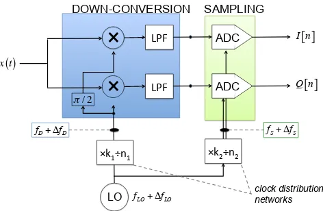
The available specifications do not provide the exact details in all the levels of the RTL-SDR hardware architecture [4]. For our work we have assumed the general architecture depicted in Fig. 1 with a single Local Oscillator (LO) that feeds both the Down-Conversion (DC) and the Sampling (S) stage by means of two distinct clock distribution networks.
We introduce the following notation:
• fLO thenominalLO frequency.
•∆fLO(t)the difference between theactualLO frequency at
timet and its nominal value, i.e., theabsolutefrequency
offset of LO.
•γ(t)def= ∆fLO
fLO the instantaneousrelativefrequency offset of
LO at timet.
• fDthenominaltune-in frequency.
•∆fD(t)the difference between theactualand nominal
tune-in frequency at timet, i.e., theabsolutefrequency offset at
the down-conversion stage.
• fSthenominalsampling rate.
•∆fS(t)the difference between theactualand nominal
sam-pling rate at timet, i.e., theabsolutefrequency offset at the
sampling stage.
In general, we can assume that therelativefrequency offset at the
down-conversion and sampling stage are equal or anyway very close to the LO one, formally:
∆fS(t)
fS ≈
∆fD(t)
fD ≈
∆fLO(t)
fLO =γ(t). (1)
LO π/ 2
fLO+ΔfLO
×
LPF ADC I n[ ]×
LPF ADC Q n[ ]×k2÷n2 ×k1÷n1
fD+ΔfD fS+ΔfS
DOWN-CONVERSION SAMPLING
clock distribution networks
x t( )
Figure 1: Reference receiver architecture.
The relative frequency offsetγ(t)is a dimension-less parameter.
The specifications typically provide an indication of the maximum LO frequency toleranceϕ expressed in parts-per-million (ppm). For example, a relative frequency tolerance of 30 ppm means a maximum time offset of 30 microseconds in one second. The tol-erance value represents an upper bound on the maximum relative deviation that may be expected, i.e.|γ(t)| ≤ϕ.
2.2
Design goals
Our goal is to develop a generic method to estimate and evaluate the frequency offset of the low-cost RTL-SDR devices with the following features:
• Reliable:The method should report a reliable estimate of the
LO frequency offset, with estimation error below 1 ppm.
• Fast: The method should be fast to provide new estimates
with a maximum delay of 1 second, in order to minimize any outage in the spectrum measurement campaign.
• Flexible:The method shall be flexible enough to work with
different RTL-SDR devices (TCXO and non-TCXO models), possibly with large LO offset values (several tens of ppm).
• Efficient:The method should be executed in small-factor
embedded architectures such as Raspberry Pi.
3
LTESS-track
In this section, we detail the proposed methodology to estimate the LO offset of SDR devices. Our method relies on the availability of LTE signals that are captured by the SDR devices.
3.1
LTE Signal model
We first briefly review a few fundamental concepts about LTE. Typically in LTE networks, the user needs to get the cell id of the base station and the frame synchronization to perform more complex operations. The first step in order to get the proper time and frequency synchronization is to search for the PSS (Primary
Synchronization Signal) and SSS (Second Synchronization Signal)
Table 1: LTE Parameters
TF 10 ms Nominal period of LTE frames. fS 1.92 MHz Nominal sampling frequency. TS 520 ns Sampling period (fS−1)
fD 806 MHz Nominal center frequency of the LTE cell∗ ∗We have tested three different LTE cells at different frequencies: 796 MHz, 806 MHz
and 816 MHz. All results were very similar. In this work we present only the results for the 806 MHz cell.
PSS and SSS signals can be found in subframes 0 and 5 of every frame. The PSS is a frequency-domain Zadoff-Chu [5] 128 bits long sequence and encodes the layer identity of the cell. The SSS encodes the cell identity and is modulated using binary phase-shift keying (BPSK). For our purposes, we consider only the PSS signal and its periodicity (twice every 10 ms) to design a frequency offset estimation method.
The choice of LTE synchronization signals as absolute clock ref-erence is motivated by the very high precision and stability of such signals: in fact, LTE base stations must meet strict requirements in terms of frequency stability with maximum tolerance below 0.05 ppm [7], i.e., much smaller than the expected tolerance of RTL-SDR devices currently on the market.
We consider the LTE parameters as shown in Table 1. The input stream of complex baseband IQ samples at the sampling ratefS
will be denoted byx[n]def=x(t)|t=nTs. We shall index ink=0,1, . . .
consecutive LTE frames. Without loss of generality, we fix the time origin at the (true) arrival time of the PSS signal for the first frame
k=0. For the generick-th frame, we denote byy[k]the true
(un-known) PSS arrival time, and by ˆy[k]the correspondingmeasured
value, as obtained with the measurement procedure detailed later in Section 3.2. Two distinct sources of errors affect the the measured value ˆy[k]: the clock errorρkand the measurement noiseek, i.e.
ˆ
y[k]=y[k]+ρk+ek=kTF+ρk+ek. (2)
The measurement noise termekis modeled by a sequence of i.i.d. random variables with zero-mean and varianceσe2. The clock
er-ror accumulated until thek-th frame is given by the integral of the instantaneous (relative) frequency deviationγ(t)and can be
developed as
ρk =∫ kTF
0 γ(t)dt≈γkTF +
∫ kTF
0
ℓ Õ
n=1
βntndt, (3)
wherein the last term represents the time-varying component of the LO frequency and is modeled (approximated) by a polynomial of sufficiently high degreeℓ. From Eq. (3) we derive the general signal model for time-varying LO frequency:
ˆ
y[k]=(1+γ) ·kTF +
ℓ+1
Õ
n=2
αnkn+ek (4)
withαn =βnTFn/n. For a short observation interval we can neglect
the time-varying component (αn=0,n=1, . . . , ℓ) and consider a
staticscenario with fixed frequency offsetγ(t)=γ. In this special
case the model simplifies as: ˆ
y[k]=(1+γ) ·kTF +ek. (5)
x n
[ ]
A: search for K consecu/ve PSSz n
[ ]
B: search for K consecu/ve PSS
C: tracking of PSS peaks ZC-128 template
adjusted template
ˆ
γ0
z'
[ ]
ny k
[ ]
Figure 2: Overview of our PSS tracking algorithm.
Consider an observation window of durationW seconds embed-dingN def=
⌊TW
F⌋frames. The vector of measurements collected in
said window will be denoted by ˆy def=
{yˆ[k],k = 1, . . . ,N}. The
choice between the static model Eq. (5) and the dynamic model Eq. (4) depends on the durationWof the observation window and on the temporal stability of the LO. For short windows of a few sec-onds, we can neglect temporal variations and resort to the simpler static model Eq. (5).
3.2
Estimation of PSS arrival times
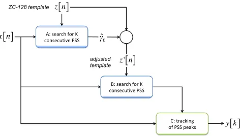
In this section, we describe the method implemented to obtain a pre-cise estimate of the (sequence of) PSS arrival times ˆy[k]. The overall
scheme is depicted in Fig. 2. The PSS tracking stage is preceded by an initial acquisition stage.
The core block of the PSS detection process is a correlation filter: a chunk ofL = 128 samples from the input IQ stream starting at positionmis correlated with the known ZC-128 templatez[n].
However, we introduce the following refinements:
• Frequency offset compensation: in order to counteract the
effect of frequency offset in the down-conversion stage, we consider the following frequency-adjusted template
z′
[n]def=z[n] ·exp−j2πγˆ0fDfS (6)
wherein ˆγ0denotes a coarse initial estimate of the frequency
offset, obtained during the initial acquisition phase.
• Up-sampling: in order to achieve sub-sample resolution for
the individual estimate ˆy[k]we up-sample the IQ stream
by a large factorU. Unless differently specified we used
U =40. For more details on the principles of re-sampling and up-sampling refer to [8].
• To speed-up the computation process, in the tracking stage
correlation and up-sampling are applied only to the portion of the incoming IQ stream in the neighborhood of the ex-pected PSS position as predicted from the previous frame, and specifically in a search window of±Nsearchsamples
centered at ˆy[k−1]+TF, withNsearch<<TFfS.
Hereafter we elaborate on the need to consider the frequency-adjusted template Eq. (6). Generally speaking, for a continuous-time signals(t), the ambiguity functionA(τ,ν)is given by the
byτ(sec) and shifted in frequency byν(Hz), formally:
A(τ,ν)def=
∫ ∞
∞
s(t) ·s∗(t−τ)exp+j2π ν tdt
(7)
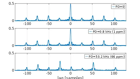
In Fig. 3(a) we plot the ambiguity function for one of the ZC-128 sequences used for PSS. The horizontal lines in the plot correspond to frequency offset values that are relevant for our experiments, namelyν1=0.8 kHz andν2=53.2 kHz. For a carrier frequency
fD = 806 MHz these values represent 1 ppm and 66 ppm CFO
(carrier frequency offset), respectively. The corresponding sections of the ambiguity function in the delay domain are plotted in Fig. 3(b). From there, it is clear the effect that a large frequency offset (66 ppm) has onto the cross-correlation function: the single large peak atτ=0 vanishes while other secondary peaks get stronger, with the effect of shifting the “highest peak" position by several sample periods. It should be noted that such a pattern will anyway occur periodically — with apparent periodγTF at the receiver —
due to the periodicity of the LTE frame structure. Since our goal is to estimate the actualrateof the PSS periodicity, and not the
absolutephaseof the periodic pattern, the delay shift introduced by
a frequency offset at the down-conversion stage does not impede by itself the estimation process. However, the reduced strength of the highest peak is detrimental to the precision of the process. For this reason, we perform an initial estimation of the frequency offset using the original templatez[k]and then compensate for the
frequency offset by considering the adjusted templatez′[k]defined
in Eq. (6) instead of the original sequencez[k](c.f. Fig. 2).
3.3
Estimation of instantaneous frequency
deviation
The overall estimation process is split into two stages:
•Estimation of PSS arrival times ˆyfrom the stream of IQ
samples, as presented in the previous subsection.
•Estimation of the instantaneous frequency offset ˆγ(or ˆγ(t)
for the dynamic case) from the vector of PSS arrival times ˆy. The latter is detailed in the present subsection.
If the observation windowWis sufficiently short, we can neglect higher-order variations of the instantaneous LO frequency (i.e., frequency drift) occurring within the observation window and consider the fixed-frequency (static) model in Eq. (5). In this case, from the vector ofN measurements ˆy[k]we obtain an estimate ˆγ
simply by linear regression. The higher the precision of individual measurements (i.e., the lowerσe), the faster a reliable estimate of ˆ
γcan be achieved. In case of longer observation windows (larger
W), we must consider the dynamic clock error model in Eq. (4). In this case, we apply higher-order polynomial regression in order to estimate the coefficients ˆγand ˆαn’s, and from the latter compute the
ˆ
βn’s. The collection of such parameters represents the full trajectory of the LO frequency within the (long) observation window.
To illustrate, in Fig. 4 we present the estimated profile of ˆγ(t)
ob-tained with real devices during an observation window of 5 minutes. The continuous line was obtained by processing all the data from the whole long window ofW=5 minutes in a single batch, with re-gression to an high-order polynomial. The red circles represent the estimates obtained by splitting the dataset into short sub-windows ofW=5 seconds, with simple linear regression based on the static
0.8 kHz 53.2 kHz
(a) Ambiguity function in the Doppler/delay plane. The horizontal lines represent the sections plotted in Fig. 3(b).
-100 -50 0 50 100
0 0.5
FO=0
-100 -50 0 50 100
0 0.5
FO=0.8 kHz (1 ppm)
-100 -50 0 50 100
lag [samples]
0 0.5
FO=53.2 kHz (66 ppm)
(b) Autocorrelation sequences for the different frequency offset values (sections of ambiguity function).
Figure 3: Ambiguity function for one ZC-128 sequence.
(a) non-TCXO “blue" (b) TCXO “silver"
Figure 4: Short-term fluctuations: the red circles represent estimates obtained with short windows of 5 sec and lin-ear regression. The continuous line represents the result of higher-order polynomial regression on the total window of 5 min.
(a) Raspberry-Pi (b) TCXO “Silver" (c) Non-TCXO “Blue"
Figure 5: Hardware
4
EVALUATION
In this section, we detail the testbed used and explain the com-parison made by LTESS-track against three open source tools for frequency offset estimation.
4.1
Testbed
We deploy an outdoor testbed to perform the evaluation of the frequency offset for different RTL-SDR devices. We rely on the Raspberry-Pi (RBPi) as the main board (Fig. 5(a)) to execute the different tools in a Linux environment. We setup a set of RBPis in a small container with TCXO RTL-SDR devices (Fig. 5(b)) and non-TCXO RTL-SDR devices (Fig. 5(c)) attached to enable the com-parison among the different frequency estimation methods. In ad-dition to that, we also measure the ambient temperature and the temperature of the RTL-SDR case (with commercial temperature sensors) in order to study their relation with the frequency offset.
4.2
Evaluated tools
The following three existing tools have been considered for this study in addition to the newly proposed method:
•rtl_test[3]. This benchmark tool is part of the rtl-sdr
soft-ware. The simple approach used for rtl_test is to count the samples read by the RTL-SDR device and compare it with the nominal sampling rate.
•Kalibrate-RTL[1]. This tool allows to scan and find GSM
base stations in a frequency range and therefore use them to estimate the frequency offset of the rtl-sdr local oscillator.
•LTE-Cell-Scanner[2]. This tool performs a LTE base
sta-tion search in a given frequency range. Once the base stasta-tion is detected the tool reports the cell id and the frequency off-set estimated using the PSS and SSS defined in LTE structure [11, Chapter 7] [5].
We evaluate each tool described above against our LTESS-track. As it is detailed below, we found some common limitations among those tools in terms of coarse time granularity, long processing time and, in some cases, gross estimation errors.
Comparison with rtl_test. The main limitation of the rtl_test
tool is the coarse temporal resolution. This tool computes the fre-quency offset based on the difference between the actual number of IQ samples collected in each time-bin of durationωinterval[0,ω]
and the expected number thereof based on the nominal sampling frequency. This method is affected by errors in the determination
0 2 4 6 8 10 12
time (minutes)
45 50 55 60 65 70 75
fr
eq. offset (ppm)
rtl_test (window=5s) rtl_test (window=15s) rtl_test (window=30s) rtl_test (window=60s) LTESS-track (window=1s)
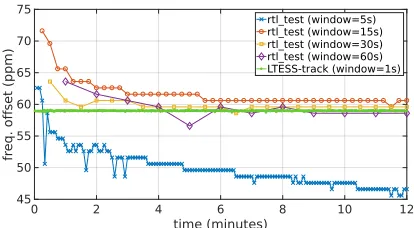
Figure 6: Comparison with rtl_test (non-TCXO).
of the reference intervalω in the absence of an accurate refer-ence clock. rtl_test introduces a new source of error which is the frequency offset of the internal clock of the computer where the measurement is performed. In order to mitigate this error, two pos-sible approaches can be taken: (1) choose a large value forW, and (2) averageksubsequent measurements. The temporal resolution of the measurements is thereforeτdef=k
·ω. Fig. 6 shows the estimated
LO frequency offset values reported by rtl_test afterτseconds based on the average ofksubsequent measurements in window of sizeW, for different values of the latter. The measurement obtained with our method is also plotted as reference. It can be seen that even with the most favorable setting (W =60 sec), it takes more than 3 minutes for rtl_test to approach the LO offset value as determined by LTESS-track after 1 sec. Furthermore, withW=5 sec the output values appear to be diverging. We conclude that rtl_test cannot be used to evaluate frequency offset variations at timescales smaller than a few minutes.
Comparison with Kalibrate-RTL. We observed that this tool
delivers grossly erroneous results when used with devices affected by large frequency offsets. For example, for the “blue" non-TCXO dongle, it was reporting an estimated value of ˆγ=−22 ppm while
all other tools where consistently reporting values around ˆγ = +59 ppm. The inaccuracy of this tool when applied on devices with LO offsets in excess of about 20 ppm is a known issue1. The problem can be mitigated by providing a good initial guess of the LO frequency offset as input to the tool. That means Kalibrate-RTL can be used only to refine the initial estimate obtained by other means. In Fig. 7, we report the estimated values obtained with Kalibrate-RTL for different initial guess values given as input. It should be noted that even with proper initialization, the reported output value is sensitive to the exact input value.
Comparison with LTE-Cell-Scanner. Next, we tested
LTE-Cell-Scanner. Similarly to our new tool, also LTE-cell-track relies on LTE signals as reference. This tool uses a fixed observation window of 160 ms and this is the value that we used in our tests. For most of the measurement timebins, the reported value were very close to the one estimated by our method—a clear indication of the precision of both tools. However, in less 1% of the timebins we observed occasional large errors (see Fig. 9(a) and Fig. 9(b)). Another limitation of this tool is the heavy computation: on a RPi-3 it takes approximately 1 minute to process the data and report a frequency
0 2 4 6 8 10 12 time (minutes)
-20 0 20 40 60
fr
eq.
offset
(ppm) Kalibrate-RTL (initial_ppm=0)
Kalibrate-RTL (initial_ppm=40) Kalibrate-RTL (initial_ppm=80) LTESS-track
Figure 7: Comparison with Kalibrate-RTL (non-TCXO).
0 10 20 30 40
time (minutes)
57 58 59 60 61 62
fr
eq. offset (ppm)
(a) Non-TCXO “Blue"
0 10 20 30 40
time (minutes)
-2 -1 0 1
fr
eq. offset (ppm)
(b) TCXO “Silver"
0 10 20 30 40
time (minutes)
30 35 40
temperat
ur
e (ºC)
non-TCXO rtl-sdr TCXO rtl-sdr
(c) Sensors temperature
Figure 8: Short-term frequency offset variations for Non-TCXO (top) and Non-TCXO (middle) RTL-SDR devices. Sensors temperature is shown on the bottom.
offset estimation. Due to such limitations, it is not possible with this tool to observe frequency offset fluctuations at small timescales.
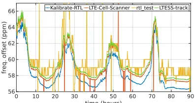
0 10 20 30 40 50 60 70 80 90
time (hours) 56
58 60 62 64 66
fr
eq. offset (ppm)
Kalibrate-RTL LTE-Cell-Scanner rtl_test LTESS-track
(a) Non-TCXO “Blue": Frequency offset vs time
0 10 20 30 40 50 60 70 80 90 time (hours)
-1 -0.5 0 0.5 1 1.5 2
fr
eq. offset (ppm)
Kalibrate-RTL LTE-Cell-Scanner rtl_test LTESS-track
0 10 20 30 40 50 60 70 80 90
-10 -5 0 5 10
(b) TCXO “Silver": Frequency offset vs time
0 10 20 30 40 50 60 70 80 90
time (hours)
20 30 40 50 60
temperat
ur
e (ºC)
non-TCXO rtl-sdr TCXO rtl-sdr Ambient
(c) Temperature vs time
Figure 9: Long-term frequency offset analysis.
4.3
Short-term variations
In Fig. 8(a) and Fig. 8(b), we plot the evolution of the LO frequency offset estimated with LTESS-track. We run our method during the first 40 minutes of operation (starting from a cold state of the de-vices), respectively, for the blue and silver dongles. Fig. 8(c) shows the device temperature. An initial transitory state is clearly in place, with steeper LO frequency excursion due to initial heating. After approximately 20 min the device temperature stabilizes (around 40◦C) and so does the LO frequency. For the non-TCXO dongle, we
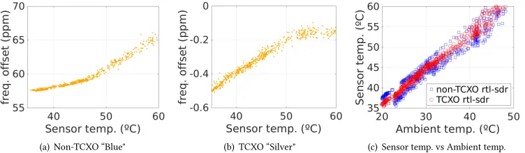
(a) Non-TCXO “Blue" (b) TCXO “Silver" (c) Sensor temp. vs Ambient temp.
Figure 10: Frequency offset and temperature analysis.
4.4
Long-term variations
We have conducted a set of long-term measurements to evaluate LO offset variations of the RTL-SDR devices over a long period and across different temperatures, and at the same time to perform a long-term comparison of the output of different tools. The different tools were run on the same device in a round-robin fashion, with cycles of 10 minutes during a measurement period of 90 hours. In order to perform a fair comparison we have configured each tool to work in the most favorable conditions. More specifically: 1) rtl_test runs duringτ=4 minutes and averaging the cumulative frequency offset estimation everyω=1 minute; 2) Kalibrate-RTL executes taking as input the initial offset estimation as computed by LTESS-track in the previous time-bin; 3) LTE-Cell-scanner executes with default configuration (recall that the computation time is about 1 minute in the Raspberry-Pi). 4) LTESS-track is configured with an observation window ofW=1 second.
Fig. 9(a) shows the frequency offset estimates reported in each cycle of 10 minutes by the different tools for the non-TCXO "Blue" device. The first observation is that the frequency offsets in these devices are strongly depending on the temperature: the higher the temperature, the higher the instantaneous LO frequency, as can be seen more clearly in Fig. 9(c). LTESS-track and LTE-Cell-Scanner report very similar values except that the second one occasionally estimates the frequency offset with a large error. Kalibrate-RTL shows a similar trend of the frequency offset estimated but with a gap in the order of 1-2 ppm. Recall from Fig. 7 that the output values of this tool are somewhat dependent on the initial guess provided in input. It seems that the precision of this tool is some-what limited to 1-2 ppm. By last, rtl_test reports very inaccurate frequency offset values even using the most favorable settings, with observation intervals of 4 minutes. Notice also that the resolution of the estimates provided by rtl_test is 1 ppm.
The long-term results for the TCXO "Silver" RTL-SDR device are shown in Fig. 9(b). The rtl_test tool again reports grossly in-accurate offset values (peaks of±10 ppm and average around -4
ppm). that the minimum resolution is 1 ppm. However the other 3 tools (Kalibrate-RTL, LTE-Cell-Scanner and LTESS-track) report similar values<1 ppm. Kalibrate-RTL shows a higher gap com-pared to our method (0.5 ppm), but as said above, the precision of this tool is anyway coarser than 1 ppm. LTE-Cell-Scanner shows again occasional large errors (maximum peaks of -9 ppm). Besides those, we observe a small and systematic gap of 0.2 ppm between
the estimates delivered by LTE-Cell-Scanner and LTESS-track that could be caused by minor differences in the computation details between the two tools.
In Fig. 10(b), we plot the frequency offset of the TCXO RTL-SDR device as reported by LTESS-track versus the device temperature. The plotted data points span the whole measurement period of 90 hours. We can conclude that the stability of the TCXO device is well within the specifications (<1 ppm). Notice that up to 50◦C
there is an approximately linear relation between frequency offset and temperature while in the range of 50-60◦C the frequency offset
remains constant. On the other hand, non-TCXO RTL-SDR devices (Fig. 10(a)) shows an absolute frequency offset of several tens of ppm (50-70) with daily fluctuations around±5 ppm depending on the
temperature. By last, Fig. 10(c) shows the linear relation between the temperature in the ambient and the temperature on the RTL-SDR device during operation. Both TCXO and non-TCXO devices seem to be 15◦C above the temperature of the environment.
4.5
Computation performance
We have evaluated the execution time of every tool by measuring the time required to compute one single LO offset estimate. The tests are performed in a Quad-Core i5 laptop. LTE-Cell-Scanner reads samples for 160 ms and then computes a single frequency offset measurement in 15 seconds, due to the heavy computations needed for the PSS and SSS detection. However, LTESS-track is optimized for LO estimation and is able to provide a frequency offset measurement every second (reading samples for 0.5 seconds). LTESS-track is also 10 times faster than Kalibrate-RTL which per-forms each frequency offset measurement every 10 seconds. The evaluation of the rtl_test performance is not relevant since the per-formance depends on the the observation window, and the latter is 4 minutes long for this tool (besides the frequency offset estimated is not reliable).
5
CONCLUSIONS
computational cost and linear regression of samples. Our method is 10 times faster than the best open-source tools currently available, and is able to provide a new estimate every second. Therefore, our method allows to analyze and evaluate short-variations in time of the frequency offset. We have evaluated the two most common RTL-SDR devices in the market, the ones with TCXO integrated and the ones without. We have demonstrated that the frequency offset of the LO can be highly temperature dependent. Thanks to LTESS-track we can conclude that the maximum fluctuation in the TCXO "silver" device is around 0.2 ppm, while the non-TCXO "blue" device reports daily fluctuations of±5 ppm around an average
value that can be in the order of 50-70 ppm. LTESS-track can be extended to work with any SDR front-end capable of tuning to LTE frequencies. The advantages of our approach become significant in crowd-sourced scenarios where LO frequency offsets need to be estimated quickly and compensated for a massive number of RTL-SDR devices deployed over a wide area. The MATLAB im-plementation of LTESS-track is released as open-source2. We are
currently working towards an optimized implementation in C/C++ designed to work with Raspberry-Pi.
REFERENCES
[1] 2012.kalibrate-rtl. https://github.com/steve-m/kalibrate-rtl.
[2] 2012.LTE-Cell-Scanner. https://github.com/Evrytania/LTE-Cell-Scanner. [3] 2016.rtl_test. https://github.com/steve-m/librtlsdr.
[4] 2016.Silver v3 specifications. http://www.rtl-sdr.com/buy-rtl-sdr-dvb-t-dongles/. [5] Evolved Universal Terrestrial Radio Access. 2016. Physical channels and
modula-tion.3GPP TS36.211 (2016), V8.
[6] Ayon Chakraborty, Md Shaifur Rahman, Himanshu Gupta, and Samir R Das. 2017. SpecSense: Crowdsensing for Efficient Querying of Spectrum Occupancy. InIEEE INFOCOM.
[7] ETSI. 2013.Evolved Universal Terrestrial Radio Access (E-UTRA); Base Station (BS) radio transmission and reception (3GPP TS 36.104).
[8] Fred J. Harris. 2004.Multirate Signal Processing for Communication Systems. [9] S. Rajendran, R. Calvo-Palomino, M. Fuchs, B. Van den Bergh, H. Cordobés, D.
Giustiniano, S. Pollin, and V. Lenders. 2017. Electrosense: Open and Big Spectrum Data. (2017). https://arxiv.org/abs/1703.09989
[10] M. Schäfer, P. Leu, V. Lenders, and J. Schmitt. 2016. Secure Motion Verification using the Doppler Effect.Proc. of the 9th ACM Conference on Security & Privacy in Wireless and Mobile Networks.
[11] S. Sesia. 2011.LTE - The UMTS Long Term Evolution: From Theory to Practice. [12] M. Strohmeier, M. Schäfer, M. Fuchs, V. Lenders, and I. Martinovic. 2015. OpenSky:
A Swiss Army Knife for Air Traffic Security Research. InProceedings of the 34th IEEE/AIAA Digital Avionics Systems Conference (DASC).