Centralized Unmanned Aerial Vehicle (UAV) Mesh
Networks Placement Scheme: A Multi-Objective
Evolutionary Algorithm Approach
Sérgio Sabino1,2,* , António Grilo1,2
1 Instituto Superior Técnico-Universidade de Lisboa; Av. Rovisco Pais 1, 1049-001, Lisboa, Portugal 2 INESC-ID; R. Alves Redol 9, CP 1000-100, Lisboa, Portugal, [email protected]
* Correspondence: [email protected]; Tel.: +351-969-356-209
Academic Editor: name
Version October 16, 2018 submitted to Preprints
Abstract: In the past, Unmanned Aerial Vehicles (UAVs) were mostly used in the military operations 1
to prevent pilot losses. Nowadays, the fast technological evolution enables the production of a class 2
of cost-effective UAVs which can service a plethora of public and civilian applications, specially 3
when configured to work cooperatively to accomplish a task. However, designing a communication 4
network among the UAVs is challenging task. In this article, we propose a centralized UAV placement 5
strategy, where UAVs are used as flying access points forming a mesh network, providing connectivity 6
to ground nodes deployed in a target area. The geographical placement of UAVs is optimized based 7
on a Multi-Objective Evolutionary Algorithm (MOEA). The goal of the proposed scheme is to cover 8
all ground nodes using a minimum number of UAVs, while maximizing the fulfillment of their data 9
rate requirements. The UAVs can employ different data rates depending on the channel conditions, 10
which are expressed by the Signal-to-Noise-Ratio (SNR). In this work, elitist Non-Dominated Sorting 11
Genetic Algorithm II (NSGA-II) is used to find a set of optimal positions to place UAVs, given the 12
positions of the ground nodes. We evaluate the trade-off between the number of UAVs used to cover 13
the target area and the data rate requirement of the ground nodes. Simulation results show that the 14
proposed algorithm can optimize the UAV placement given the requirement and the positions of the 15
ground nodes in the geographical area. 16
Keywords:Unmanned Aerial Vehicles, Genetic Algorithm, Mesh Networks, Optimization, MOEA, 17
NSGA-II 18
1. Introduction 19
Unmanned Aerial Vehicles (UAVs), also known as drones refer to aircrafts with no human pilot 20
on board. These are either programmed and fully autonomous or remotely and fully controlled 21
from another location, e.g., ground or space station. There are various types of UAVs (e.g., Fixed 22
wing and multi-rotor) and they come in different sizes, raging from small (less than 5 kg) to large 23
(over 4332 kg) [1]. Large UAVs are commonly used singly , for instance, in military operation such 24
as border surveillance, strike and reconnaissance, whereas small UAVs may be utilized in swarms 25
to accomplish a mission. With advancement in electronics and sensor technology, small UAVs are 26
becoming massively present in many public and civilian application, such as in search and rescue 27
operations [2], aerial surveillance [3], tracking targets[4], agriculture field monitoring [5], network 28
extension or compensation [6], leisure, to mention a few. 29
The use of swarms of small UAVs has many advantages compared to a single and large UAV [7]. 30
One of the key advantages is the cost to acquire and maintain small UAVs, which is generally much 31
lower than the cost of a large UAV [8]. Swarms of UAVs can automatically reconfigure themselves 32
in a case of node failure or link break, and accomplish the designated task. That is not possible with 33
a single UAV. Additionally, when network coverage extension is needed, it may be easily achieved 34
with swarms of UAVs by positioning additional UAVs in the target area and allow them to operate 35
through other already existing UAVs, unlike single UAV network coverage which is limited by the 36
communication range between the infrastructure and the UAV itself. 37
Although swarms of UAVs present many advantages, an important aspect to be considered when 38
designing an application using multiple UAVs is the communication network, which poses many 39
challenging issues as described in [9]. Depending on the purpose of the application at hand, UAVs may 40
be semi-stationary and hovering over the area of operations or move around at high speed changing 41
their relative positions. In the latter scenario, frequent topology changes are observed, which may 42
lead to network partitioning and poor link quality. On the other hand, the commonly used wireless 43
ad-hoc network communication protocols or algorithms (e.g., proactive and reactive routing) cannot be 44
directly used for UAVs [10]. For instance, since proactive routing protocols need to update the routing 45
tables periodically, in the presence of high degree of mobility and topology changes, it increases the 46
number of control messages to be exchanged, which degrade the network performance. On the other 47
hand, reactive protocols may introduce higher packet delivery delay each time they compute a new 48
route to the destination node. 49
UAV placement schemes can help to mitigate the aforementioned issues by finding suitable 50
positions to place UAVs while maintaining connectivity and improving the network performance. 51
The UAV placement optimization schemes can be classified as centralized or distributed. The former 52
assumes that the UAV positions are selected by a centralized entity and conveyed to the UAVs by 53
means of special purpose long-range low bit rate radio interface. On the other hand, in distributed 54
approaches, UAVs work cooperatively to adjust their position based on local interactions to achieve 55
optimal coverage. This work extends our previous work [11], where we considered the use of a swarm 56
of UAVs as flying access points forming a mesh network among themselves, providing connectivity to 57
ground nodes (GNs). Our main goal is to optimize the placement of the UAVs by choosing deployment 58
positions for the UAVs in order to provide adequate wireless communication coverage to GNs in a 59
target area, while fulfilling their Quality of Service (QoS) requirements. 60
This work is more related with centralized placement optimization. It considers the following 61
requirements and constraints: 62
• Minimization of the number of UAVs needed to service the GN, while ensuring that the QoS 63
requirements (here measured as the physical data rate) are properly met. 64
• The number of available UAVs is limited and must not be exceeded; 65
• The inter-UAV links do not necessarily employ the same technology as GN-UAV links. Inter-UAV 66
links are considered in an abstract way, but constrained to a maximum range. 67
• It is assumed that the throughput values of the links between UAVs are high enough not to 68
constrain end-to-end inter-GN traffic. Only GN-UAV links impose limits to the satisfaction of 69
QoS requirements (end-to-end QoS shall be addressed in future work); 70
• GN-UAV links are orthogonal. This can be achieved, for example, by assigning different 71
frequencies or orthogonal channel codes. 72
Given the nature of the problem requirements, we consider using Multi-Objective Evolutionary 73
Algorithm (MOEA) techniques to optimize the UAV node placement considering two main objectives, 74
namely, to minimize the number of UAVs and the degree of dissatisfaction regarding the required data 75
rate. 76
The paper is structured as follows. Section 2 presents the related work. In Section 3 the system 77
model is presented. Section 4 presents the problem definition and formulation as a Multi-Objective 78
Optimization Problem (MOP). Section 5 presents our MOAEA implementation. The simulation results 79
are presented in Section 6. Section 7 presents the simulation results discussion and Section 8 concludes 80
the paper. 81
2. Related Work 82
Optimal placement of UAVs has already been studied in the literature whether considering single 83
as earthquake, flood or bomb blast. The goal is to deploy an UAV to a position where it can bridge 85
communication between two static nodes on the ground. It is assumed that the UAV hovers the area 86
in spiral or ladder search mode sending hello/beacon messages in regular interval. Upon receiving 87
such a message, the GNs respond by sending their GPS positions back to the UAV. The UAV stores 88
this information and continues hovering in the immediate surrounding to find a position based on the 89
received signal strength (RSS) and distance between the UAV and nodes on the ground. Simulation 90
results showed that the algorithm provides maximum throughput and low bit error rate (BER) once 91
the UAV is fixed at an optimal position. The drawback of this system is that it is only validated for two 92
GNs. Therefore, as the number of GN grows, the solution should consider energy constraints during 93
the search process and bandwidth constraints when providing network access to GNs. 94
The authors in [12] have developed a framework named UAVNet. It is capable to autonomously 95
deploy a wireless mesh network to interconnect two end systems using small quadrocopter-based 96
UAVs with 802.11s nodes on board. Each UAV would act as access point and provides network access 97
for regular IEEE 802.11g wireless devices. There are two positioning modes to place the UAVs between 98
the end systems.The first one is the location based positioning mode. The latter uses the submitted 99
GPS locations of the end systems and directs the UAV to the exact geographical position between these 100
two GPS coordinates. The second one is the signal strength positioning mode. It extends the location 101
positioning mode and includes also the received signal strength of the two end systems to calculate a 102
more accurate position for the UAV. This takes the quality of the wireless link and other environmental 103
factors into account. 104
Usually, the process of network densification in cellular networks uses fixed small cells (e.g., 105
picocells and fentocells) to increase the network capacity based on the expected formation of hotspots. 106
In places where temporary hotspots are formed, fixed small cells would remain under-utilized once 107
the hotspots moved to a different location or disappeared. Authors in [13] proposed small cells 108
mounted on UAVs to offload user equipments (UEs) from the microcell infrastructure. The optimum 109
placement points of the UAVs are determined using K-means clustering algorithm. In their work, the 110
performance metric where measured based on the RSS experienced by the UEs. The simulation results 111
have shown that as UAVs are able to position themselves in real-time around actual UE position rather 112
than expected UE hotspots, they outperform equivalent small cell deployment. 113
In [14], the authors present a model for an optimal placement of UAVs to cover a set of targets, i.e., 114
GNs. They consider two cost metrics, namely, the number of UAV and energy consumption, seeking to 115
minimize both metrics. The authors assume that each UAV has a minimum and maximum observation 116
altitude. They also assure that the UAV’s energy consumption is related to this altitude, since the 117
higher the altitude, the larger the observed area, but also the higher the energy consumption. The 118
optimization problem is mathematically solved by defining an integer linear and a mixed non-linear 119
optimization model. 120
The authors in [15] use the same assumption as in [14] to model an optimized UAV placement and 121
formulate it as a multi-objective linear problem. The main difference is that, in [15], the connectivity 122
among UAVs is considered as an additional constraint. In [15], the following objectives are to be 123
minimized: number of UAVs and the maximum flying altitude. Our work is closer to [15] though 124
with some differences. Firstly, we consider using omnidirectional antennas instead of directional. 125
Secondly, one of our objectives is to minimize the difference between the assigned and required data 126
rate, whereas one of their objectives is to maximize the flying altitude. 127
3. System Model 128
We consider a wireless network consisting of two kinds of nodes, GNs and UAVs, which are represented by the setsVandU, respectively. All nodes are assumed to be located in a rectangular area
Awith lengthXmaxand widthYmax. Nodes are equipped with omnidirectional transceivers and a GPS.
uis represented in the 3D plane asqu(x,y,h), wherehis the flying altitude ofu. We assume that the main factor which affects the service quality offered by an UAV is path loss, as it is assumed that the links between a GN and its serving UAV are line-of-sight (LOS) links. We employ the free-space propagation model given by the Friis equation, as follows:
PR=PTGTGR
λ 4πd
2
(1)
wherePRis the received power,PT is the transmission power,GTandGRare the transmitter
and receiver antenna gains, respectively.λ= cf represents the wavelength of the carrier wave, where
cis the speed of light and f is the carrier wave frequency. UAVs are assumed to have the same operating characteristics, featuring the same transmit power, antenna gains and altitude. GNs can only communicate with each other through UAVs. The parameterdin Equation (1) represents the distance between the transmitter and receiver antennas of the nodes. Assuming communication between a GN and an UAV,dis computed as the Euclidean distance between their transceivers as follows:
d=
q
(xu−xv)2+ (yu−yv)2+h2u (2)
The distancedshould not be greater than the maximum communication rangeD. We computeD
based on the receiver sensitivity, denoted asPRSdBm. ConsideringGT =GR=1 (0dBm) in Equation (1), it yields:
D=10
PTdBm−PRSdBm−20 log(f) +147.56
20 (m) (3)
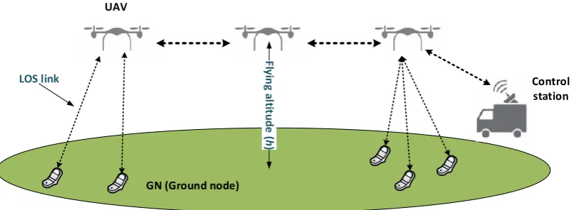
An overview of the proposed system is shown in Figure1. 129
UAV
GN (Ground node)
LOS link
Fly
in
g a
lti
tu
d
e
(
h
)
Control station
Figure 1.System model overview.
4. Problem Definition 130
Consider the network model presented in Section3. The goal is to ensure that all GNs are covered 131
and that the data rate requirements are met as much as possible when UAVs are used as relay nodes. 132
We assume that there is a cost associated with each used UAV. Thus, minimizing the number of UAVs, 133
is desirable. On the other hand, GNs may have different data rate requirements. The satisfaction 134
of data rate as GN requirements is closely dependent on the channel conditions (e.g., SNR), which 135
also depends on the communication distance, which results from the number and placement of the 136
serving UAV in the network. We intend to deploy as few connected UAVs as possible in suitable 137
locations to enable communication between GNs, while satisfying multiple independent data rate 138
simultaneously. This gives rise to the need of finding solutions that try to balance them. This problem 140
can be modelled meta-heuristically as a multi-objective optimization problem to find the trade-off 141
among non-dominated solutions. In the rest of this section, we define Multi-Objective Optimization 142
Problem (MOP) and present the formulation of our UAV placement optimization problem as a MOP. 143
4.1. Multi-Objective Optimization Problem (MOP)
144
A MOP can be stated as follows [16]:
minimizeF(ε) = (f1(ε), ....fm(ε))
subject toε∈Ω
(4)
WhereΩis thedecision (variable) space,<mis theobjective space, andF : Ω → <mconsist ofm 145
real-values objective functions. IfΩis a closed and connected region in<mand all the objectives are 146
continuous ofε, we call Equation (4) a continuous MOP. 147
4.1.1. Domination 148
Letk= (k1, ....,km), l = (l1, ....,lm) ∈ <mbe two vectors,kis said todominate lifki ≤lifor all 149
i=1, ....,mandk6=l1. 150
4.1.2. Pareto front 151
A pointε∗ ∈ Ωis called(Globally) Pareto optimalif there is noε∈ Ωsuch thatF(ε)dominates 152
F(ε∗). The set of all the Pareto optimal points, denoted byPS, is called thePareto set. The set of all 153
Pareto objective vectors,PF={F(ε)∈ <m|ε∈PS}, is called thePareto front. 154
4.2. Formulation of UAV Placement Optimization as a MOP
155
In this section we formulate the problem inR2objective space. We seek to minimize the number 156
of deployed UAVs and simultaneously minimize the difference between the data rate required by the 157
GNs to transmit data and the data rates that results from the MOP solution. 158
4.2.1. Minimize the number of UAVs 159
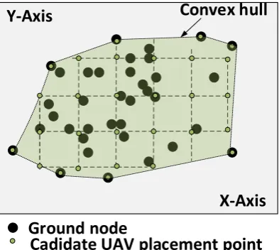
We start by identifying a set of potential UAV placement pointsQ, by finding a sub-areaa0 ⊂ A
160
which corresponds to the area inside the convex hull (convex envelope) [17] formed by the GNs inA
161
as shown in Figure2. We compute the convex hull to reduce the search space of the UAVs placement 162
points in the target area. We intend to cover all GNs ina0. Therefore, we discretizea0in a grid layout 163
according to Equation (5). 164
1 This definition of domination is for minimization. All the inequalities should be reversed if the goal is to maximize the
Ground node
Cadidate UAV placement point
Y-Axis
X-Axis
Convex hull
Figure 2.Convex hull formed by the GNs.
αD;α∈[0, 1] (5)
whereαadjusts the distance between two neighboring UAVs. Letqj ∈ Qbe thejthpotential UAV 165
placement point. We defineδuqj as a binary variable to indicate which points are currently being used 166
by an UAV as presented bellow. 167
168
δquj =
1 if UAVuis located atqj
0 Otherwise 169
We also defineζuvas a binary variable to indicate which GNs are being serviced by each deployed 170
UAV. It is assumed that a GN will be connected to the closest deployed UAV. 171
172
ζuv =
1 ifvis connected to UAVu 0 Otherwise
173
Our objective is to select points inQsuch that 174
min
∑
qj∈Q
∑
u∈U
δuqj (6)
subject to:
∑
qj∈Q
δquj ≤1,∀u∈U (7)
∑
v∈V
ζuv≥1,∀v∈V (8)
Constraint (7) indicates that each UAVucannot be placed in more than one point at the same 175
time. Constraint (8) ensures that a GN is at communication range of at least one UAV. The cardinality 176
of the setQdefines the maximum number of UAVs that can be used for each formed convex hull. In 177
order to ensure connectivity among UAVs, we have considered using the Algorithm1, which verifies 178
assumed to have two main attributes: serving, when the UAV is used to serve GNs and to connect the 180
network, and bridging when it is solely being used to connect the serving UAVs. 181
Algorithm 1Construction of connected UAV network. 1: Input:udest, adjacency matrix
2: Result: Connected UAV network 3: For eachu∈U
4: IF uis serving anduis not bridging
5: qcurr=qu; /*qcurr∈Qis the current point toward destination*/ 6: Untilnot reachable(u,udest)
6.1 Find the closest pointq0 ∈Qtoqudestwhich is whitin distanceDfromqcurr 6.2If q0is not in use
6.2.1 qcurr=q0
6.2.2 Findu0∈Uwhich is not serving or bridging 6.2.3 Set:u0to bridging
6.2.4 qu0 =qcurr
6.2.5 Update adjacency matrix
4.2.2. Minimizing the degree of dissatisfaction of the required data rate 182
Consider a set of transmission modes B comprising the possible bit ratesbi. We denote the
transmission modes in use by an UAV and requested by a GN asbui andbvi, respectively. We define the degree of dissatisfaction as follows:
γv=
|bui −bvi|
bvi if(b
u
i −bvi)<0
0 Otherwise
(9)
We consider that the use of abidepends on the SNR. Usually, GNs experiencing a relatively low 183
SNR will have their receiver interface tuned to a robust (with lower BER when compared with other 184
modes under the same channel conditions) transmission mode with lower data rate. On the other 185
hand, if SNR is relatively high, the receiver may be tuned to a transmission mode which offers higher 186
data rate. In this work, we try to minimize the maximum dissatisfaction value as follows: 187
min(maxv∈Vγv) (10)
5. UAV placement based on NSGA-II 188
In this section we present terminologies used by NSGA-II [18] and the main genetic algorithm 189
elements (individual or chromosome, fitness, selection, population and genetic operators). The term 190
solutions and individuals are interchangeably used along the remaining part of this paper. 191
NSGA-II is an elitist MOEA which comprises two main procedures. One is the Pareto ranking 192
procedure, which aims at sorting the population into different non-domination levels (irank) in 193
ascending order. The lowest ranking level contains the best solution. In order to identify solutions of 194
the first non-dominated front in a population of sizeN, each solution is compared with every other 195
solution in the population to find if it is dominated. After all members of the first non-dominated 196
front are found, they are discounted temporally so that the next non-dominated front could be found 197
by repeating this first procedure. The other procedure is the diversity preservation which is used to 198
maintain a good spread of solutions in the obtained set of solutions. Members in each non-dominated 199
of solutions surrounding a particular solution in the population. A solution with a smaller value of this 201
distance measure is, in some sense, more crowded by other solutions. Thecrowded-comparison operator, 202
denoted as≺n, is used to distinguish the best solution during selection process. It assumes that every 203
individualiin the population has two attributes,irankandidistance. The partial order≺nis defined as: 204
i≺n jif(irank<jrank)
or((irank =jrank)and(idistance>jdistance))
(11)
That is, between two solutions with differing non-domination ranks, we prefer the solution with 205
the lower (better) rank. Otherwise, if both solutions belong to the same front, then we prefer the 206
solution that is located in a less crowded region. 207
Algorithm2shows the main loop of NSGA-II proposed by the authors in [18], where the call of 208
the routinesfast-non-dominated-sort(Rt) andcrowding-distance-assignment(Fi) corresponds to the first 209
and second procedure described above, respectively. Rtis of size 2Nformed by combining parent 210
St and offspringZt populations. Fi refers to theith front or level. The detailed explanation of the 211
aforementioned procedures is also available in [18]. We describe the main loop of NSGA-II as follows: 212
Algorithm 2NSGA-II main loop. 1: Rt=St∪Zt
2: F=fast-non-dominated-sort(Rt)
3: St+1=∅andi=1 4: Until|St+1|+Fi ≤N
4.1. crowding-distance-assignment(Fi)
4.2.St+1=St+1+Fi
4.3.i=i+1 5: Sort(Fi,≺n)
6: St+1=St+1∪ Fi[1 :(N− |St+1|)] 7: Zt+1=make-new-pop(St+1) 8: t=t+1
Step 1. Combine parent and offspring population; 213
Step 2.F = (F1,F2, ...), sortRtaccording to non-domination procedure; 214
Step 3. Initialize an empty set for the parent populationPt+1=∅and set a counterito 1;
215
Step 4. Until the parent population is filled; 216
4.1. Calculate crowding-distance inFi; 217
4.2. Includeithnon-dominated front in the parent pop; 218
4.3. Check the next front for inclusion. Best solutions are inF1. If the size ofF1is smaller 219
thanN, we choose all the members of the setF1for the new populationSt+1. The remaining
220
members of the populationSt+1are chosen from subsequent non-dominated front in the
221
ascending order of their ranking,(F2,F3, ...). Say that the setFlis the last non-dominated 222
set beyond which no other set can be accommodated. In general, the count of solutions in 223
all sets fromF1toFlwould be larger than the population size. In order to choose exactlyN 224
population members, we sort the solutions of the frontFl using the crowded-comparison 225
operator(≺n)in descending order and choose the best solution needed to fill all population 226
slots; 227
Step 5. Sort in descending order using≺n; 228
Step 6. Choose the first(N− |St+1|)elements ofFi; 229
Step 7. Use selection, crossover and mutation to create a new populationZt+1;
230
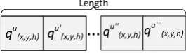
5.1. Individual
232
An individual encodes a candidate solution to the problem. Our proposed individual stores the 233
UAVs positionsqu
j ∈Qinside the discretized convex hull areaa0for each deployed or serving UAV. 234
The length of the individual (see Figure3) represents the number of deployed UAVs or points used in 235
Q. If it is detected that some GNs are not covered, then the corresponding individual is considered as 236
invalid, i.e., cannot be used in any step of NSGA-II algorithm. Algorithm1ensures that all individuals 237
are valid during the creation of initial population. 238
qu(x,y,h) qu'(x,y,h)
Length
qu(x,y,h) qu'(x,y,h) q u''
(x,y,h)qu'''(x,y,h)
...
Figure 3.Individual.
5.2. Initial population
239
The initial population is a set ofNrandomly generated valid individuals. 240
5.3. Objective or fitness function
241
A fitness function decodes the solution represented by a chromosome and let us know how far 242
we are from the optimal/ideal solution if it is known. In MOEA there will be a fitness function for 243
each objective space. Equations (6) and (10) compute the fitness for the number of UAVs and degree of 244
dissatisfaction, respectively. Values scored from both objective functions are used by NSGA-II to set 245
theithfront. 246
5.4. Selection
247
The goal of selection procedure is to pick the best individuals to the next generation. We use 248
binary tournament selection based on crowded-comparison operator≺nas described in Section5. 249
5.5. Genetic Operators
250
Genetic operators are responsible for generating new solutions to populate the next generations. 251
In the next sections we present how they are performed. 252
5.5.1. Crossover 253
Two parents are chosen to exchange their genes with a probabilitypc. We rely on 2D representation 254
of each parent (see Figure4) to show how crossover is conducted. In this procedure, we find the 255
midpoint ina0 and draw a separation or cutting line to divide the area in two parts in each of the 256
parents. The cutting line may be drawn diagonally in 45/-45 degrees or horizontally or vertically. 257
Next, we remove all UAVs that are within12Ddistance radius along the cutting line withina0. If the 258
separation line is either diagonally or vertically drawn, the leftmost part of one parent is joined with 259
the rightmost part of the other to form an offspring. On the other hand, if it is horizontally drawn, the 260
uppermost and bottommost will be joined instead. There may be some uncovered GNs in the vicinity 261
of the separation line, since we have removed some UAVs, which makes the resulting offspring an 262
invalid individual. In this case, we repair the offspring by repeatedly choosing a random uncovered 263
GN and place an UAV in a closest available pointqu
(x,y,h)until all GNs are covered and connectivity
264
among UAVs is verified by the Algorithm1. UAVs which are not serving or bridging any GNs are 265
Ground node Parent A
UAV coverage radius
Parent B
Offspring
Crossover point
Figure 4.Crossover procedure
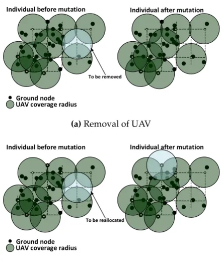
5.5.2. Mutation 267
For each individual an UAV is randomly chosen based on a probabilitypm. Next, either it is 268
temporally removed from the network or reallocated to a new available placement point with 50% 269
chance for each procedure to be performed. If the above procedures fail to produce a valid individual, 270
then the UAV is put back in its initial position. Figures5aand5bshow the removal and reallocation 271
procedures, respectively. 272
Ground node UAV coverage radius
Individual before mutation Individual after mutation
To be removed
(a)Removal of UAV
Ground node UAV coverage radius
Individual before mutation Individual after mutation
To be reallocated
(b)Reallocation of UAV
6. Simulation results 273
In this section, we present simulation results of our implementation of NSGA-II. We have two 274
objective functions. The first one aims at reducing the cost in term of the number of deployed 275
UAVs used to service GNs, and the second one is intended to reduce the maximum dissatisfaction 276
of GNs in term of the required data rate. We have developed the algorithm in C++ programming 277
language. The setup of the proposed scenarios, the MOEA termination criterion and the dominated 278
and non-dominated sets are presented in section6.1,6.2and6.3, respectively. 279
6.1. Scenario setup
280
We considered a network with 120 fixed GNs uniformly distributed in a rectangular area of size 281
10000 m×10000 m. We set three different scenarios by varying the value ofα. This parameter is used 282
to discretize the area inside the convex hull formed by the GNs. Differently from our previous work 283
[11] where UAVs were only allowed to fly at fixed altitude, here an UAV may fly at a given altitudeh
284
uniformly selected from the setH= {40, 80, 120} m. We assume that the transmit power among the 285
nodes is fixed at 23 dBm. Previously, in section4, it was stated that potential UAV placement points 286
will be identified within a convex hull formed by the GNs. The convex hull is found by the Graham 287
scan algorithm [19] based on the GN deployment positionsqv
(x,y,0). Table1shows all possible data rates
288
and their corresponding minimum sensitivities. These values were used to compute the maximum 289
achievable distanceDigiven by equation3. Moreover, each data rate in Table1is considered to be 290
using a different transmission mode. 291
Table 1. Calculation of the maximum achievable distance of each transmission mode based on the minimum sensitivity of the receiver antenna.
Data Rate (Mbits/s) Min. Sensitivity (dBm) Di(m)
6 -82 1760.93
9 -81 1569.43
12 -79 1246.64
18 -77 990.24
24 -74 701.04
36 -70 442.32
48 -66 279.08
54 -65 248.73
Our scenarios considers free space path loss for the signal attenuation. For the set of UAV 292
candidate positionQ, we choseDiwith the lowest minimum sensitivity and adjust it by using the 293
parameterαto ensure that two UAVs positioned side by side can communicate with each other. As 294
already stated, we assume that there is a wireless communication technology between UAVs that is 295
capable of efficiently relaying all the traffic from the GNs, never causing a bottleneck. The parameters 296
that are common in different scenario are detailed in Table2as follows: 297
Table 2.Parameters in each scenario.
Parameters Value
Transmit Power 23 dBm
Antenna model Omni-directional Propagation model Free space AreaA, (Xmax×Ymax) 10000 m×10000 m
Nr. of GNs 120
c 3×10⁸m/s
f 2.412×10⁹Hz
α [0.15, 0.30, 0.45]
We have adjusted NSGA-II parameters such as, the probability of crossover and mutation and the 298
population size so that the algorithm does not prematurely converge or perform excessive number of 299
computation due to either low values of the probability of crossover or high population size. NSGA-II 300
parameters are summarized in Table3. 301
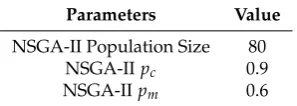
Table 3.NSGA-II setup parameters.
Parameters Value
NSGA-II Population Size 80
NSGA-IIpc 0.9
NSGA-IIpm 0.6
6.2. MOEA termination criterion
302
The MOEA termination adopted in this work is similar to that used in [20], in the sense that 303
we also maintain an external archive of non-dominated solutions obtained at some predefined steps 304
at earlier generations, and it is subject to be updated some generations later. However, instead of 305
computing the ratio of the number of solutions in the archive that are dominated by the new ones of 306
the current generation and the ratio of the number of solutions that are also present in the new set 307
of non-dominated solutions, we compute the ratio of new solutions which are not present in both 308
dominated and non-dominated sets of the archive and we use it to define our stopping criterion. We 309
usee=0.05 as cut-off value for the new solutions. However, the choice of the exact cut-off value may 310
depend on the problem and may require some trial and error. Figure6shows the ratio of new solutions 311
at every tenth generation (i.e., step=10). The ratio was significantly high in the first generation when 312
the algorithm was evolving and decreased with the generation as new solutions were not frequent. 313
We also observe that depending onαthe NSGA-II takes different number of generation to achieve 314
the cut-off value. In fact, the value ofαaffects the cardinality ofQhence increasing or decreasing the 315
search space, i.e., the higher the cardinality ofQthe higher is the number of generations to achieve the 316
cut-off value. On the other hand, the lower the cardinality ofQthe lower is the number of generation 317
to achieve the cut-off value. These results are shown in Table4. 318
Table 4.Number od generations achieved for cut-offe=0.05 for eachα.
α=0.15 α=0.30 α=0.45
# of generations 190 179 151
6.3. Dominated and non-dominated sets
319
For each value ofα, all dominated and non-dominated solutions are presented in Figure7. From 320
each Pareto front set, we can clearly see the trade-off between the number of UAVs that are flying in 321
the area and the degree of dissatisfaction of the GNs in terms of the required data rate, i.e., when few 322
UAVs are deployed, a high degree of the maximum dissatisfaction is observed. On the other hand, 323
when the number of UAVs increases, the degree of the maximum dissatisfaction decreases. 324
(a)α=0.15 (b)α=0.30
(c)α=0.45
Figure 7.Trade-off between the number of UAV and the degree of dissatisfaction of the GNs
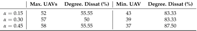
Table5presents the maximum and minimum number of UAVs and their respective degrees of 325
dissatisfaction from the Pareto front set of each value ofαpresented in Figure7. These results show 326
that the proposed algorithm can optimize the UAV placement given the requirement and the positions 327
Table 5.Maximum and minimum nr. of UAVs for each scenario.
Max. UAVs Degree. Dissat (%) Min. UAV Degree. Dissat (%)
α=0.15 52 55.55 43 83.33
α=0.30 57 50 39 83.33
α=0.45 58 55.55 37 87.50
7. Discussion 329
As shown above varyingαaffects the objective functions, though we have computed the convex 330
hall to reduce the search space to some extent. However, this parameter may still reduce or increase 331
the number of candidate points to place UAVs in the target area. The choice ofαdepends on the 332
requirement such as the area to be covered, the maximum transmission range, and also the number of 333
available UAVs to cover the GNs to meet the QoS requirements. 334
The use of NSGA-II as an optimization tool allows us to produce a set of solutions which are 335
better and spread as observed in our simulations results. It enables us with options to select a solution 336
according to the requirement of the application or problem at hand. For instance, if it is not acceptable 337
that any GN communicates beyond 75 % of degree of dissatisfaction and there are no more than 60 338
available UAVs , then they can easily be configured with solutions that respect these requirements 339
from our Pareto-optimal (non-dominated) set chosen from Figure7. 340
The experimental results presented in previous section are specific to the proposed scenarios and 341
assumptions which were considered in our system model. In a realistic environment, one should take 342
into account additional constraints such as the effect of interference, GN mobility, number of GNs to 343
be covered, terrain conditions, etc. 344
• Interference: Nodes may be positioned within acceptable distance for the required data rate, but 345
may fail to achieve it due to interference caused by ongoing transmission of their neighboring 346
nodes. 347
• GN mobility: Although the mobility is not considered in this work, it is worth to mention that it 348
would at least demand scheduling of periodic updates and computation of new solutions due to 349
topology changes. As was previously mentioned, that is a challenging issue, namely because of 350
the need to minimize temporary connectivity disruption due to UAV position changes. 351
• Number of GNs:UAVs have a limited capacity to efficiently service a certain number of GNs, if 352
this capacity is exceed, additional UAVs may be needed. 353
• Terrain conditions/ structure:UAV may not fly at desired altitude due to the existence of obstacles 354
(e.g., trees, mountains, buildings, etc.), which may require the addition of more UAVs to maintain 355
the connectivity among the nodes. 356
Algorithm1was used to ensure the connectivity of the network and produce valid solutions. We 357
use breadth first search (BFS) algorithm to check if there is a path to the destination. If a path is not 358
found, it adds a new UAV to connect it as explained in Section4.2.1. This procedure is not optimized, 359
which may conflict with the objective of minimizing the number of UAVs. However, it may eventually 360
reduce the degree of dissatisfaction of the GNs. 361
8. Conclusions 362
This paper presents an optimized placement scheme for UAV access points providing network 363
connectivity to GNs with differentiated data rate requirements. The goal of the proposed algorithm is 364
to deploy as few as possible connected UAVs to cover and simultaneously satisfy the aforementioned 365
requirements of the GNs. In order to attain this goal, we have mathematically formulated the problem 366
and used a MOEA named NSGA-II to run the simulations. In order to NSGA-II to work we proposed 367
a chromosome structure, crossover scheme and mutation procedure. Simulations were performed 368
mode within a set of available ones. Simulation results show that the algorithm optimizes the UAV 370
placement given the requirements and positions of the GNs, considering the trade-off between the 371
number of UAVs and quality of the coverage. 372
In future work we will consider additional constrains such as limited inter-UAV link capacity. We 373
will also consider joint topology and routing optimization. 374
Acknowledgments:This work was partially supported by Fundação Calouste Gulbenkian and by Portuguese 375
national funds through Fundação para a Ciência e Tecnologia (FCT) with reference UID/CEC/50021/2013. 376
Conflicts of Interest:The authors declare no conflict of interest. 377
Abbreviations 378
The following abbreviations are used in this manuscript: 379
380
BER Bit error rate BFS Breadth first search
GN Ground node
GPS Global positioning system
IEEE Institute of electrical and electronics engineer MOEA Multi-objective evolutionary algorithm MOP Multi-objective optimization problem NSGA-II Non-dominated sorting genetic algorithm II QoS Quality of service
PS Pareto set
RSS Received signal strength SNR Signal-to-noise-ratio UAV Unmanned aerial vehicles
UE User equipment
Wi-Fi Wireless fidelity 381
References 382
1. K. Dalamagkidis, K. P. Valavanis, and L. A. Piegl, “Current status and future perspectives for unmanned 383
aircraft system operations in the us,”Journal of Intelligent and Robotic Systems, vol. 52, no. 2, pp. 313–329, 2008. 384
2. H. Ullah, S. McClean, P. Nixon, G. Parr, and C. Luo. An optimal uav deployment algorithm for bridging 385
communication. InITS Telecommunications (ITST), 2017 15th International Conference on, pages 1–7. IEEE, 386
2017. 387
3. R. W. Beard, T. W. McLain, D. B. Nelson, D. Kingston, and D. Johanson. Decentralized cooperative aerial 388
surveillance using fixed-wing miniature uavs.Proceedings of the IEEE, 94(7):1306–1324, 2006. 389
4. L. Reynaud and I. Guérin-Lassous. Design of a force-based controlled mobility on aerial vehicles for pest 390
management. Ad Hoc Networks, 53:41–52, 2016. 391
5. H. Xiang and L. Tian. Development of a low-cost agricultural remote sensing system based on an autonomous 392
unmanned aerial vehicle (uav). Biosystems engineering, 108(2):174–190, 2011. 393
6. S. Rohde, M. Putzke, and C. Wietfeld. Ad hoc self-healing of ofdma networks using uav-based relays. Ad 394
Hoc Networks, 11(7):1893–1906, 2013.
395
7. I. Bekmezci, O. K. Sahingoz, and ¸S. Temel, “Flying ad-hoc networks (fanets): A survey,”Ad Hoc Networks, 396
vol. 11, no. 3, pp. 1254–1270, 2013. 397
8. K. Anderson and K. J. Gaston, “Lightweight unmanned aerial vehicles will revolutionize spatial ecology,” 398
Frontiers in Ecology and the Environment, vol. 11, no. 3, pp. 138–146, 2013.
399
9. L. Gupta, R. Jain, and G. Vaszkun, “Survey of important issues in uav communication networks,”IEEE 400
Communications Surveys & Tutorials, vol. 18, no. 2, pp. 1123–1152, 2016.
401
10. J. Jiang and G. Han, “Routing protocols for unmanned aerial vehicles,”IEEE Communications Magazine, 402
11. S. Sabino and A. Grilo, “Topology control of unmanned aerial vehicle (uav) mesh networks: A multi-objective 404
evolutionary algorithm approach,” inProceedings of the 4th ACM Workshop on Micro Aerial Vehicle Networks, 405
Systems, and Applications. ACM, 2018,pp. 45–50.
406
12. S. Morgenthaler, T. Braun, Z. Zhao, T. Staub, and M. Anwander, “Uavnet: A mobile wireless mesh network 407
using unmanned aerial vehicles,” inGlobecom Workshops (GC Wkshps), 2012 IEEE. IEEE, 2012, pp. 1603–1608. 408
13. B. Galkin, J. Kibilda, and L. A. DaSilva, “Deployment of uav-mounted access points according to spatial user 409
locations in two-tier cellular networks,” inWireless Days (WD), 2016. IEEE, 2016, pp. 1–6. 410
14. D. Zorbas, L. D. P. Pugliese, T. Razafindralambo, and F. Guerriero. Optimal drone placement and cost-efficient 411
target coverage.Journal of Network and Computer Applications, 75:16–31, 2016. 412
15. C. Caillouet and T. Razafindralambo. Efficient deployment of connected unmanned aerial vehicles for 413
optimal target coverage. InGlobal Information Infrastructure and Networking Symposium (GIIS), 2017, pages 414
1–8. IEEE, 2017. 415
16. H. Li and Q. Zhang. Multiobjective optimization problems with complicated pareto sets, moea/d and 416
nsga-ii. IEEE Transactions on evolutionary computation, 13(2):284–302, 2009. 417
17. R. A. Jarvis. On the identification of the convex hull of a finite set of points in the plane.Information processing 418
letters, 2(1):18–21, 1973.
419
18. K. Deb, A. Pratap, S. Agarwal, and T. Meyarivan. A fast and elitist multiobjective genetic algorithm: Nsga-ii. 420
IEEE transactions on evolutionary computation, 6(2):182–197, 2002.
421
19. R. L. Graham. An efficient algorith for determining the convex hull of a finite planar set. Information 422
processing letters, 1(4):132–133, 1972.
423
20. T. Goel and N. Stander, “A study of the convergence characteristics of multiobjective evolutionary 424
algorithms,” in13th AIAA/ISSMO Multidisciplinary Analysis Optimization Conference, 2010, p. 9233. 425