Article
1
Watershed-scale surface runoff and water quality
2
response to climate change, urbanization, and
3
implementation of LIDs
4
Mohammad Nazari-Sharabian 1, * Moses Karakouzian 2 and Sajjad Ahmad 3
5
1 Ph.D. Candidate, Department of Civil and Environmental Engineering and Construction, University of Nevada
6
Las Vegas, Las Vegas, USA; [email protected]
7
2 Professor, Department of Civil and Environmental Engineering and Construction, University of Nevada
8
Las Vegas, Las Vegas, USA; [email protected]
9
3 Professor, Department of Civil and Environmental Engineering and Construction, University of Nevada
10
Las Vegas, Las Vegas, USA; [email protected]
11
12
* Correspondence: [email protected]
13
14
Abstract: The Storm Water Management Model (SWMM) was used to evaluate the impact of
15
urbanization, climate change, and implementation of Low Impact Developments (LIDs) at the
16
Mahabad Dam watershed, Iran. Several scenarios of urbanization, with and without climate change
17
impacts, in different locations were defined, including near outlet, middle, far end, and whole
18
watershed. Climate change was considered to change the intensity of rainfall and increase
19
evaporation. Vegetative swales were implemented as LIDs to evaluate their applicability to reduce
20
pollutant loads. Digital Elevation Model (DEM) of the area was input into ArcGIS, and the
21
watershed was delineated using the ArcSWAT extension to identify topographic features. Water
22
quality properties were defined in the software, and each scenario was run for a twelve-hour
23
simulation. The results indicated that urbanization affects the imperviousness of sub-catchments,
24
and location of urbanization affects the amount and timing of runoff and pollutant yields.
Fifty-25
percent urbanization near the watershed outlet resulted in 23.1% and 27.4% increases in runoff and
26
pollutant loads, respectively. Fifty-percent urbanization in the middle resulted in 28.8% and 35.4%
27
increases in runoff and pollutant loads; and, at the far end, 23.1% and 3.9% increases in runoff and
28
pollutant loads were the result; Fifty-percent urbanizing the whole watershed gave 58.6% and 66.3%
29
increases in runoff and pollutant loads, respectively; Under climate change scenarios (higher
30
intensity, shorter duration rainfall) peaks occurred earlier. Moreover, results showed LIDs
31
decreased pollution loads up to 25%.
32
Keywords: Urbanization; Climate Change; SWMM; LID; Runoff; Water Quality
33
34
1. Introduction
35
Land development is strongly related to imperviousness, which is a critical property for
36
determining surface runoff in an area. Analyzing how surface runoff may vary depending on changes
37
in the imperviousness of the land can help in making decisions to manage development so that it
38
does not cause excessive runoff and ultimately lead to higher pollutant loads, which damages
39
ecosystems in the receiving water bodies. Moreover, climate change will affect the hydrological cycle
40
and change atmospheric and meteorological properties, such as precipitation patterns, atmospheric
41
water vapor, and evaporation [1—4]. Sediment yield and nutrient losses occur as water pollutants
42
are affected by spatial and temporal alterations in precipitation patterns and precipitation intensity,
43
as well as land-use practices, land management, and population pressure.
44
Understanding how pollutants travel in an environment requires analyses of the underlying
45
hydrologic processes. The previous work of hydrologists has yielded several mathematical models
46
that can analytically describe some of the processes in this cycle. Based on these mathematical models,
47
a variety of hydrologic computer models have been developed since the Stanford Watershed Model
48
(SWM) was first introduced in 1966. Among these models is the Storm Water Management Model
49
(SWMM). The appropriateness of these models may vary depending on the characteristics of the
50
study area and user objectives.
51
In 2014, [5] evaluated the runoff reduction performance of permeable pavement systems using
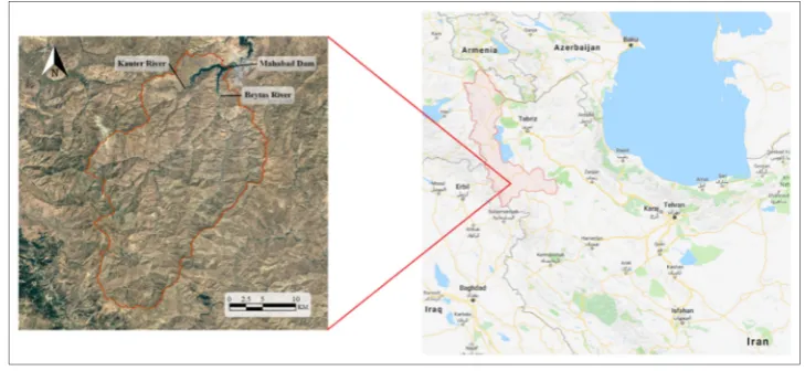
52
the low-impact development (LID) module of the widely used Storm Water Management Model
53
(SWMM) through example applications with rainfall data from Atlanta. The authors found that when
54
the depth of the pavement layer is less than 120 mm and the computational time steps are longer than
55
30 min, the method of calculating infiltration through the pavement layers of permeable pavement
56
systems in the LID module are inadequate.
57
Employing the SWMM model, [6] simulated urban flooding of Dongguan City in southern
58
China. They observed no flooding under the 1-year return period precipitation, but for the 2, 5, 10
59
and 20-year return periods of precipitation, the simulations showed that the area would be
60
inundated.
61
Moreover, in order to provide a solution to the storm water management problem in a small
62
urbanized area in West Bengal, India, [7] used the 1D SWMM and the 2D MIKE URBAN models to
63
design an efficient drainage system for the study area. The authors also designed a multi-purpose
64
detention pond for groundwater recharge and attenuating the peak of the outflow hydrograph at the
65
downstream end during high-intensity rainfall. This study provided an insight into the importance
66
of 2D models to deal with location-specific flooding problems.
67
More recently, [8] provided a method to determine pollutant buildup and washoff parameters
68
in a semi-arid Texan urban watershed, using inverse modeling. The authors calibrated hydraulic and
69
pollutant parameters, using Shuffled Complex Evolution – University of Arizona (SCEUA).
70
Additionally, the confidence intervals of pollutant parameters were calculated by GLD (Generalized
71
Lambda Distribution). The modeling results showed that buildup parameters were clustered in
72
narrow numerical ranges, indicating that spatially uniform factors were responsible for pollutant
73
buildup. Washoff parameters did not cluster and were distributed more evenly, indicating the strong
74
influence of local factors, such as topography.
75
Furthermore, [9] assessed the historical and future land-use/land-cover dynamics in the River
76
State region of the Niger Delta. In order to perform land-use classification and change detection
77
analysis, multi-source (Landsat TM, ETM, polygon map, and hard copy) data of the study area for
78
the years 1986, 1995, and 2003, as well as projected conditions for 2060 were used. The authors
79
concluded that historical urbanization was rapid, and due to planned urban development, urban
80
expansion could increase by 80% in 2060; moreover, 95% of the conversions to urban land occurred
81
chiefly at the expense of agricultural land, which in the future could amplify flood risk and have
82
other severe implications for the watershed.
83
The Mahabad Dam reservoir in Iran is suffering from year-round eutrophication caused by
84
excess nutrient loadings from the watershed. Moreover, due to land-use changes and the degradation
85
of vegetation in this watershed, the soil has become very erodible, making it vulnerable to
high-86
intensity rainfall events. In this situation, the soil wash can increase sediment yield and nutrient
87
loadings, making the reservoir’s eutrophic condition even worse. Over the past decades,
88
meteorological records have shown temperature rises and precipitation declines in the region.
89
Therefore, it is expected that in changing climate conditions, with possible further anthropogenic
90
changes in this area, the water quality of the reservoir will be affected.
91
Therefore, through implementing the SWMM model, this study intends to examine the surface
92
runoff generation and water quality characteristics in the Mahabad Dam watershed, under several
93
scenarios based on urbanization and climate change. This study, however, will limit the scope of
94
water quality analysis to pollutants, such as total suspended solids (TSS), total nitrogen (TN) and
95
total phosphorous (TP), which enter the streams from areas with different land use practices.
Ultimately, the findings of this study can be used as a guide for urban development that is in
97
accordance with environmental quality standards.
98
2. Materials and Methods
99
2.1. Case Study and Data
100
Mahabad Dam watershed is located in West-Azerbaijan province in the northwest of Iran
101
(36°44′N, 45°39′E), and is one of the Urmia Lake basins. The watershed covers an approximate area
102
of 808 km2 (199,661 ac) and is mostly covered by agricultural fields and grasslands. The Kauter and
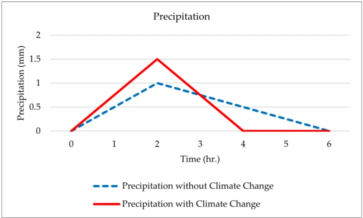
103
Beytas rivers originate from the southern heights of the plain and run to the north in parallel. They
104
join and create the Mahabad Dam reservoir and continue running as the Mahabad River (Figure 1).
105
106
Figure 1. Geographical location of Mahabad Dam.
107
In the watershed, the soil is mainly composed of Taconic and Benson. The composition of each
108
soil type in detail, and the percent coverage of the watershed area are presented in Table 1.
109
Table 1. Soil types in the Mahabad Dam watershed.
110
Soil Type Sand (%) Silt (%) Clay (%) Watershed Area (%)
Taconic 43 35 23 72
Benson 35 37 30 28
111
Fortunately, the data for several necessary parameters are freely available in the form of
112
Geographic Information System (GIS) raster data layers derived from satellite imagery. These layers
113
can be processed in GIS so that particular parameter values can be extracted and input to SWMM. In
114
this regard, a digital elevation model (DEM) of this area with 30m spatial resolution was downloaded
115
from the ASTER database, to delineate the watershed in GIS and, subsequently, to create the model
116
in SWMM.
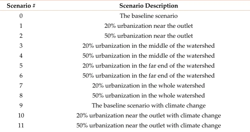
117
2.2. The SWMM Model
118
The Storm Water Management Model (SWMM) [10] is a dynamic model used for single-event
119
to long-term simulation of the surface/subsurface hydrology quantity and quality from primarily
120
urban/suburban areas. The hydrology component of SWMM operates on a collection of
sub-121
catchment areas divided into impervious and pervious areas, with and without depression storage,
122
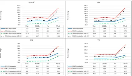
in order to predict runoff and pollutant loads from precipitation, evaporation, and infiltration losses
123
from each of the sub-catchments. The routing or hydraulics section of the SWMM transports this
124
water and possible associated water quality constituents through a system of closed pipes, open
125
channels, storage/treatment devices, ponds, storages, pumps, orifices, weirs, outlets, outfalls, and
126
other regulators. The SWMM tracks the quantity and quality of the flow generated within each
catchment, as well as the flow rate, flow depth, and quality of water in each pipe and channel during
128
a simulation period composed of multiple fixed or variable time steps. The water quality constituents
129
can be simulated from buildup on the sub-catchments through washoff to a hydraulic network with
130
optional first-order decay and linked pollutant removal. Best management practices (BMPs) and
low-131
impact development (LID) removal and treatment can be simulated at selected storage nodes [11].
132
2.3. Conceptual Design and Layout
133
In the SWMM, the hydrologic network is created by adding visual objects in the graphical user
134
interface. These visual objects include both human artifacts, like weir gates, pumps, and reservoirs,
135
and natural features, such as drainage basins and streams. The SWMM version 5.1.013 was utilized
136
in this study. There are four types of visual objects that will comprise the model of the Mahabad Dam
137
watershed: sub-catchments, conduits, junctions, and rain gage. The first step in creating the hydrologic
138
network is to determine the number of sub-catchments that will comprise the watershed. An elevation
139
map is required to determine the number of sub-catchments. Therefore, a digital elevation model
140
(DEM) of the area in a raster data format was downloaded and input into ArcGIS.
141
An ArcGIS extension called ArcSWAT was then used to delineate all of the sub-catchments of the
142
Mahabad Dam watershed based on the DEM. The following graphics show the conversion from a GIS
143
map to the SWMM graphical user interface, which includes junctions and conduits (Figure 2).
144
145
146
Figure 2. (a) Delineated watershed in ArcSWAT (b) the watershed configuration in SWMM.
147
Table 2 shows how GIS delineated sub-catchments were grouped in order to have a fewer
148
number of sub-catchments in SWMM.
149
Table 2. Sub-catchments in GIS and SWMM
150
GIS Delineated Sub-Catchments Grouped Sub-Catchments
1, 2 1
7, 9 2
3, 4, 5, 6, 8, 10, 12, 18 3
11, 13, 14 4
15, 16, 17, 19, 20, 21, 27, 31 6
22, 28, 30, 32, 33, 34 7
24, 26, 28, 36 8
35, 37, 38, 39, 40, 41, 42, 43, 44, 45 9
151
After drawing the SWMM network, the properties for each visual object has to be input. The
152
processes for determining the values of these properties are presented in the following subsections.
153
2.4. GIS-Defined Properties
154
In ArcToolbox, the area of each polygonal feature, i.e., sub-catchments, can be tabulated. These
155
area values can then be easily input as the sub-catchment properties in the SWMM. A summary of
156
all the values derived from the GIS-defined sub-catchment properties is presented in Table 3. The
157
amount of imperviousness was determined based on the approximate percent urbanization in each
158
sub-catchment.
159
Table 3. GIS-defined sub-catchment properties
160
161
162
163
164
165
166
167
168
169
170
2.5. Manning’s n and Depth of Depression Storage
171
Manning’s n value describes the resistance of an area for water to flow over it, and depends on
172
the type of land use. In this study, pervious portions of the watershedwere considered to have n
173
values equal to 0.15, while the impervious portions of the watershed were considered to have
174
Manning’s n values equal to 0.01.
175
For the impervious and pervious portions of the watershed, the depth for which precipitation
176
can pool is defined as the depth of depression storage. The pooled precipitation, thus, does not
177
become runoff. In this study, the depth of depression storage on pervious and impervious areas was
178
assumed to be 0.05 In.
179
2.6. Infiltration
180
There are several ways to estimate the amount of precipitation that infiltrates into the pervious
181
portions of the sub-catchment. In this study, the SCS Curve Number method, developed by the Soil
182
Conservation Service, was used as the infiltration method because of its simplicity. This method only
183
requires a single Curve Number value to be assigned to sub-catchments. Based on the dominant
land-184
use in the region, a Curve Number value of 80 was assigned to each sub-catchment.
185
2.7. Conduit Properties
186
The length of conduits was determined using the ArcGIS ruler tool and tracing the length of
187
each of the stream segments from the ArcSWAT derived stream network. The conduits were sized in
188
Sub-Catchment Area (ac) Width (ft) % Slope % Impervious
1 9384 16400 32 5
2 10105 16400 24 5
3 31169 26240 32 4
4 13284 16400 29 5
5 23095 26240 29 5
6 40916 32800 36 3.5
7 17033 19680 31 5
8 21462 26240 30 5
a way that no conduit surcharge happens under the most critical scenario. The list of scenarios is
189
presented in Table 7, under the scenarios subsection.
190
2.8. Junction Properties
191
Only the invert elevation, as the junction property, was considered in this study. The invert
192
elevation is simply the elevation at the junction measured from sea level. This elevation was obtained
193
from the Google Earth software. It was assumed that the maximum depth at the junction is the same
194
as the depth of the connecting stream segment. Initial depth was ignored since the results were
195
centered only on the flow from runoff and not base flow.
196
2.9. Non-Visual Objects
197
Non-visual objects do not appear in the SWMM graphical user interface, but are nevertheless
198
important components of the model, such as climatology, land-uses, pollutants, and low impact
199
developments (LIDs).
200
2.9.1. Climatology
201
A single rain gage was used to provide the rainfall data for every sub-catchment. A rainfall time
202
series shows the amount of precipitation that falls within a specified time interval. In this study, it
203
was assumed that a 3-inch rainfall event occurs in 6 hours. In the climate change scenario, it was
204
assumed that the same amount of rainfall precipitates in a shorter time period of 4 hours and has a
205
higher intensity (Figure 3). Without climate change, the evaporation rate was considered to be 80
206
mm/month (0.104 in/day), while the amount of evaporation under climate change was considered to
207
be 154 mm/month (0.2 in/day).
208
209
Figure 3. Precipitation, with and without climate change.
210
2.9.2. Land-Uses and Pollutants
211
Each land-use must have its properties defined in order to run a water quality simulation. Each
212
land-use contains a buildup and washoff function whose forms are defined by the user. The SWMM
213
allows users to define any number of pollutants, though in this study only TSS, TN and TP were
214
analyzed. The antecedent dry days were assumed to be 100. The agricultural TN and TP rate
215
constants and washoff EMCs were assumed to be twice the value of those in residential areas. The
216
buildup and washoff EMC values used in this study are presented in Table 4 and 5, respectively [11].
217
Table 4. Buildups: rate constant (lb/ac.year)
218
0 0.5 1 1.5 2
0 1 2 3 4 5 6
Precipitation (m
m
)
Time (hr.) Precipitation
Precipitation without Climate Change
Pollutant Residential
(Medium Density) Undeveloped Agricultural
TSS (Max. Build Up) 0.52 (50) 0.26 (25) 0.52 (50)
TN (Max. Build Up) 0.01068 (1) 0.00534 (0.5) 0.02137 (2)
TP (Max. Build Up) 0.00137 (0.5) 0.00068 (0.25) 0.00274 (1)
Table 5. Washoff EMCs (mg/l)
219
Pollutant Residential
(Medium Density) Undeveloped Agricultural
TSS 60 50 60
TN 3 1.7 6 TP 0.3 0.12 0.6
2.9.3. LIDs
220
LID is an approach to land development that works with nature to manage storm water as close
221
to its source as possible. In order to treat storm water as a resource rather than a waste product, LIDs
222
employ principles such as preserving and recreating natural landscape features to create functional
223
and appealing site drainage [12].
224
In this study, vegetative swales were used as the LIDs in sub-catchments undergoing
225
urbanization. It was assumed that LIDs in each sub-catchment cover 10% of the area and treat 50% of
226
runoff from developed areas and 50% of runoff from undeveloped areas. Table 6 represents the
227
properties of the LIDs used in this study.
228
Table 6. Vegetative swale properties
229
Berm Height (In.) Vegetation Volume Fraction
The Surface Roughness (Manning’s n)
Surface Slope (%)
Swale Side Slope (run/rise)
1.0 0.0 0.1 1.0 5.0
2.10. Scenarios
230
In order to determine the impact of urbanization on runoff and water quality, several scenarios
231
were proposed, which are presented in Table 7. For these scenarios, it was assumed that urbanization
232
only changes the percent of imperviousness of the sub-catchment and leaves everything else constant.
233
Table 7. Scenarios on land development
234
Scenario # Scenario Description
0 The baseline scenario
1 20% urbanization near the outlet
2 50% urbanization near the outlet
3 20% urbanization in the middle of the watershed
4 50% urbanization in the middle of the watershed
5 20% urbanization in the far end of the watershed
6 50% urbanization in the far end of the watershed
7 20% urbanization in the whole watershed
8 50% urbanization in the whole watershed
9 The baseline scenario with climate change
10 20% urbanization near the outlet with climate change
12 20% urbanization in the middle of the watershed with climate change 13 50% urbanization in the middle of the watershed with climate change 14 20% urbanization in the far end of the watershed with climate change
15 50% urbanization in the far end of the watershed with climate change
16 20% urbanization in the whole watershed with climate change
17 50% urbanization in the whole watershed with climate change
235
Table 8 presents the percentages of residential, undeveloped, and agricultural land-uses in each
236
sub-catchment before urbanization. In Table 9, the land use percentages are presented based on
237
urbanization near the outlet, in the middle, at the far end, and in the whole watershed.
238
Table 8. Land-uses before development
239
Sub-Catchment # %Residential %Undeveloped %Agricultural
1 5 65 30 2 5 65 30
3 4 86 10 4 5 90 5
5 5 90 5
6 3.5 86.5 10
7 5 85 10
8 5 65 30 9 3 77 20
Table 9. Land-uses after development
240
Near the Outlet
Sub-Catchment # %Residential %Undeveloped %Agricultural
1 20 (50) 50 (20) 30
2 20 (50) 50 (20) 30
3 20 (50) 70 (40) 10
4 20 (50) 75 (45) 5
5 5 90 5
6 3.5 86.5 10
7 5 85 10
8 5 65 30 9 3 77 20
Middle
Sub-Catchment # %Residential %Undeveloped %Agricultural
1 5 65 30
2 5 65 30 3 4 86 10
4 5 90 5
5 20 (50) 75 (45) 5
6 20 (50) 70 (40) 10
7 20 (50) 70 (40) 10
8 5 65 30
Far End
Sub-Catchment # %Residential %Undeveloped %Agricultural
1 5 65 30
2 5 65 30 3 4 86 10
4 5 90 5 5 5 90 5
6 3.5 86.5 10 7 5 85 10
8 20 (50) 50 (20) 30
9 20 (50) 60 (30) 20
Whole Watershed
Subcatchment # %Residential %Undeveloped %Agricultural
1 20 (50) 50 (20) 30
2 20 (50) 50 (20) 30
3 20 (50) 70 (40) 10
4 20 (50) 75 (45) 5
5 20 (50) 75 (45) 5
6 20 (50) 70 (40) 10
7 20 (50) 70 (40) 10
8 20 (50) 50 (20) 30
9 20 (50) 60 (30) 20
3. Results
241
In this study, each simulation was run for twelve hours. The following graphs show the impact
242
of urbanization and climate change on surface runoff generation and select water quality features.
243
Figure 4 shows the change in the runoff, TSS, TN, and TP loads received at the outlet of the watershed,
244
relative to the baseline scenario. Figure 5 represents the time that it took for each component to reach
245
the maximum value under different scenarios. Figure 6 shows how the implementation of LIDs helps
246
to reduce the pollutant loads in the watershed.
249
Figure 4. The change in the runoff, TSS, TN, and TP loads, relative to the baseline scenario.
250
251
Figure 5. Time of peak for runoff, TSS, TN, and TP.
252
253
0:00 1:12 2:24 3:36 4:48 6:00 7:12
0 1 2 3 4 5 6 7 8 9 10 11 12 13 14 15 16 17
Time
Scenario Time of Peak
Figure 6. Pollutant load reductions in the watershed after implementation of LIDs.
254
The results indicate that urbanization affects the imperviousness of the sub-catchments.
255
Consequently, as the imperviousness increases, rainfall no longer infiltrates into the ground, and
256
instead runs into streams. Conversions to urban land could amplify flood risk in the future and have
257
other severe implications for the watershed.
258
According to Figure 4, the highest increase in runoff and pollutant loads was observed under
259
scenario 8, which is 50% urbanization in the whole watershed, which creates the most critical case
260
among all scenarios. Under this scenario, relative to the baseline scenario, runoff, TSS, TN, and TP
261
loads increased by 137%, 158%, 119%, and 232%, respectively. After scenario 8, the highest increase
262
was observed under scenario 17 (50% urbanization in the whole watershed with climate change). The
263
results indicate that shorter duration precipitation events, along with increased evaporation rates,
264
decrease the cumulative watershed yields. On the other hand, the lowest increase was observed in
265
scenario 1 (20% urbanization near the outlet). Under this scenario, runoff, TSS, TN, and TP loads
266
increased by 15%, 16%, 18%, and 21%, relative to the baseline scenario, respectively. Moreover, under
267
scenario 9 (baseline scenario with climate change), 10 (20% urbanization near the outlet with climate
268
change), 12 (20% urbanization in the middle of the watershed with climate change), and 14 (20%
269
urbanization in the far end of the watershed with climate change), the watershed yields were
270
decreased.
271
Furthermore, Figure 5 indicates that during the twelve-hour simulation, the baseline scenario
272
showed the longest time for a peak in the runoff, received at the outlet of the watershed (6:08). Under
273
the same scenario, the time of peak for TSS, TN, and TP were 1:16. The highest increase in pollutants’
274
peak time can be observed under scenario 6 (50% urbanization in the far end of the watershed). Under
275
this scenario, since the urbanized area is far from the watershed outlet and the highest urbanization
276
percentage considered in this study was employed, the pollutant loads and the time of peak were
277
increased.
278
These findings indicate that the location of urbanization affects both the amount and timing of
279
runoff and pollutant loads. As an urbanized area is constructed farther away from the outlet point of
280
the watershed, the peaks occur later in time. The percentage of urbanization is another factor affecting
281
these values. As the urbanization percentage increases, more runoff and pollutants are generated.
282
Moreover, climate change also affects the watershed yields. When the rainfall intensity and
283
evaporation rates were increased under climate change conditions, the peaks occurred earlier in time.
284
Finally, according to Figure 6, after the implementation of LIDs, the highest reduction in
285
pollutant loads was achieved under scenario 16 (20% urbanization in the whole watershed with
286
climate change). This scenario shows a 25% reduction in all pollutant loads. After that, scenarios 7
287
(20% urbanization in the whole watershed), 17 (50% urbanization in the whole watershed with
288
climate change), and 8 (50% urbanization in the whole watershed) showed highest percentages of
289
reduction in pollutant loads. Furthermore, under scenario 9 (baseline scenario with climate change),
290
no pollutant load reductions were observed.
291
4. Discussion
292
In this study, the impact of urbanization, climate change, and implementation of vegetative
293
swales, as LID, on runoff and pollutant loads in the Mahabad Dam watershed in Iran, were evaluated.
294
The watershed was first delineated in ArcGIS and then modeled in SWMM Ver. 5.1.013. This study
295
covered seventeen scenarios on urbanization and climate change in different locations throughout
296
the watershed. The following are the main findings of this study:
297
298
• The percentage of urbanization affects the watershed yields. In this study, 50% urbanization
299
created higher runoff and pollutant loads in comparison with 20% urbanization. Comparing the
300
20% and 50% urbanization scenarios, 50% urbanization near the watershed outlet, resulted in
301
runoff and pollutant loads increase of 23.1% and 27.4%, respectively. Urbanization in the middle
302
of the watershed resulted in runoff and pollutant load increases of 28.8% and 35.4%. At the far
end of the watershed, urbanization resulted in runoff and pollutant load increases of 23.1% and
304
3.9%. Finally, urbanizing the whole watershed resulted in runoff and pollutant load increases of
305
58.6% and 66.3%, respectively. The change in watershed yields due to urbanization in different
306
locations is because of different sub-catchment areas, land uses, and imperviousness.
307
• The location of urbanization affects the amount of runoff, as well as pollutant loads. Areas
308
urbanized farther away from the watershed outlet have delayed peaks in runoff and pollutant
309
loads compared to urbanized areas near the outlet.
310
• Under climate change scenarios, the peaks occurred earlier in time because of the higher
311
intensity and shorter duration rainfall events.
312
• LIDs decreased the pollutant loads. The highest reductions were observed when LIDs were
313
employed in the following scenarios: 20% urbanization in the whole watershed with climate
314
change (25% reduction in all pollutant loads); 20% urbanization in the whole watershed (20%
315
reduction in all pollutant loads); and 50% urbanization in the whole watershed with climate
316
change (17% reduction in TSS and TP loads, and 8% reduction in TN load).
317
318
Based on the findings of this study, in order to reduce the pollutant loads entering the streams
319
and reservoir, the implementation of LIDs in this watershed is encouraged. Moreover, it is
320
recommended to find critical source areas in this watershed and to avoid urbanization in these areas,
321
since more imperviousness will increase the amount of pollutant loads from these areas as a result of
322
increased surface runoff. In addition, critical source areas should be the priority for the
323
implementation of LIDs. Ultimately, the findings of this study can be used as a guide for urban
324
development that is in accordance with environmental quality standards.
325
Author Contributions: conceptualization, Mohammad Sharabian; methodology, Mohammad
Nazari-326
Sharabian, Sajjad Ahmad; software, Mohammad Nazari-Sharabian, Sajjad Ahmad; writing—original draft
327
preparation, Mohammad Nazari-Sharabian; writing—review and editing, Mohammad Nazari-Sharabian,
328
Moses Karakouzian; supervision, Moses Karakouzian, Sajjad Ahmad.
329
Funding: This research received no external funding.
330
Conflicts of Interest: The authors declare no conflict of interest.
331
References
332
1. Intergovernmental Panel on Climate Change (IPCC). Climate Change 2007: The Physical Science Basis;
333
Cambridge University Press: Cambridge, UK., 2007; p. 996.
334
2. Intergovernmental Panel on Climate Change (IPCC), 2012. Managing the Risks of Extreme Events and Disasters
335
to Advance Climate Change Adaptation; Cambridge University Press: Cambridge, UK., 2012; p. 582.
336
3. Huntington, T.G. Evidence for intensification of the global water cycle: Review and synthesis. J. Hydrol.
337
2006, 319, pp. 83–95, https://doi.org/10.1016/j.jhydrol.2005.07.003.
338
4. Nazari-Sharabian, M.; Ahmad, S.; Karakouzian, M. Climate change and eutrophication: a short review.
339
Eng. Tech. Appl. Sci. Res. 2018, 8(6), pp. 3668-3672.
340
5. Zhang, S.; Guo, Y. SWMM Simulation of the Storm Water Volume Control Performance of Permeable
341
Pavement Systems. J. Hydrol. Eng. 2015, 20(8), 06014010,
https://doi.org/10.1061/(ASCE)HE.1943-342
5584.0001092.
343
6. Jiang, L.; Chen, Y.; Wang, H. Urban flood simulation based on the SWMM model. Proc. Intl. Assoc. Hydrol.
344
Sci. 2015, 368, pp. 186-191, https://doi.org/10.5194/piahs-368-186-2015.
345
7. Bisht, D. S.; Chatterjee, C.; Kalakoti, S.; Upadhyay, P.; Sahoo, M.; Panda, A. Modeling urban floods and
346
drainage using SWMM and MIKE URBAN: A case study. Nat. Hazards 2016, 84(2), pp. 749-776,
347
https://doi.org/10.1007/s11069-016-2455-1.
348
8. Tu, M.; Smith, P. Modeling Pollutant Buildup and Washoff Parameters for SWMM Based on Land Use in
349
a Semiarid Urban Watershed. Water Air Soil Pollut. 2018, 229(4), https://doi.org/10.1007/s11270-018-3777-2.
350
9. Dan-Jumbo, N.; Metzger, M.; Clark, A. (2018). Urban Land-Use Dynamics in the Niger Delta: The Case of
351
Greater Port Harcourt Watershed. Urban Sci. 2018, 2(4), p. 108, https://doi.org/10.3390/urbansci2040108.
352
10. Storm Water Management Model. Available online:
353
11. Storm Water Management Model User's Manual Version 5.1.
355
12. Urban Runoff: Low Impact Development. Available online:
356