Development and Verification of the Three-Dimensional
Electrostatic Particle Simulation Code for the Study of Blob and
Hole Propagation Dynamics
∗)Hiroki HASEGAWA
1,2)and Seiji ISHIGURO
1,2)1)National Institute for Fusion Science (NIFS), National Institutes of Natural Sciences (NINS), Toki 509-5292, Japan
2)Department of Fusion Science, SOKENDAI (The Graduate University for Advanced Studies), Toki 509-5292, Japan
(Received 31 May 2017/Accepted 28 September 2017)
The three-dimensional (3D) electrostatic particle-in-cell (PIC) simulation code for the study of blob and hole propagation dynamics has been developed and verified. The developed 3D-PIC code simulates the boundary layer plasma of magnetic confinement devices, and plasma particles in the simulation systems are distributed to form the blob or hole structures. For the verification, the theoretical blob and hole propagation speeds have been estimated, and the observed blob and hole propagation speeds in the simulations have been compared with the estimations. The observed relations between the propagation speed and the structure size in the blob and hole cases are in good agreement with the theoretical relations. The 3D-PIC code has reproduced a larger distortion of a hole shape than that of a blob shape. Furthermore, the code has shown that the propagation of a blob or a hole is faster without end plates. Such a situation is similar to the detached state.
c
2017 The Japan Society of Plasma Science and Nuclear Fusion Research
Keywords: blob, hole, scrape-offlayer transport, particle-in-cell simulation DOI: 10.1585/pfr.12.1401044
1. Introduction
The blob and the hole, which are intermittent fila-mentary coherent structures along the magnetic field line, are universally observed in the boundary layer plasmas of various magnetic confinement devices [1, 2]. Such struc-tures are considered to play an important role in the ra-dial transport in the boundary layer plasmas. The width of such structures is considered to be in meso-scale. In other words, the width of a small blob or a small hole is slightly larger than the ion Larmor radius. The microscopic, that is, the kinetic effects on blob and hole dynamics should be investigated because of such situations. Thus, we devel-oped the three-dimensional (3D) electrostatic particle-in-cell (PIC) simulation code called “p3bd” (particle-in-particle-in-cell 3-dimensional simulation code for boundary layer plasma dynamics) in order to study the kinetic effects on blob dy-namics [3–5]. Since the sheath potential in the vicinity of the end plate or the wall is reproduced in the p3bd code, we are able to investigate the sheath effects on blob dy-namics by using the code. In this study, we have updated the p3bd code in order to investigate the dynamics of hole (holes are thought to transport impurity ions [6–8]) and we have verified the code by comparison with the theoretical estimation of blob and hole dynamics. In Sec. 2, we briefly describe the simulation methodology. In Sec. 3, we derive the theoretical estimation of blob and hole propagation
dy-author’s e-mail: [email protected]
∗)This article is based on the invited talk at the 33rd JSPF Annual Meeting
(2016, Tohoku)
namics from the fluid model. In Sec. 4, we show the blob and hole dynamics simulated by the p3bd code and com-pare simulation results with the theoretical estimation. We summarize our work in Sec. 5.
2. Particle Simulation Code
The p3bd code is the electrostatic 3D-PIC code for the study of boundary layer plasma dynamics. In the code, the full plasma particle (electron and ions) dynamics (in-cluding the Larmor gyration motion) are calculated in 3D space and 3D velocity coordinates for all particles with the equations of motion,
dus,j dt =
qs ms
E(xs,j)+us,j×B(xs,j)
, (1)
and dxs,j
dt =us,j, (2)
wherexs,jis a position of a particle in 3D space,us,jis a 3D velocity of a particle, the subscripts sand jrepresent the species of a particle and the number of a particle, respec-tively,qsandmsare the charge and mass of speciess, and
E(xs,j) andB(xs,j) are the electric and magnetic fields on the particle position. Here, the value of a particle position has a real (continuous) number (not a discrete number).
As shown in Ref. [9], after particles are accelerated by Eq. (1) and moved by Eq. (2), the charge densityon each discrete spatial grid point is calculated from the positions
c
2017 The Japan Society of Plasma
of all particles by the charge assignment as ns(xα,β,γ)=
j
S(xs,j−xα,β,γ), (3)
and
(xα,β,γ)= s
qsns(xα,β,γ), (4)
in PIC simulation codes. Here,nsis the density, xα,β,γ is the position of the grid whose numbers in the x,y, andz directions areα,β, andγ, andS is the form-factor of the finite-size particle. Then, the electric potentialϕis solved with Poisson’s equation,
∇2ϕ=−
ε0
, (5)
by the fast Fourier transform (FFT) [10] whereε0 is the permittivity. Here, the magnetic field is constant in time because of the electrostatic code. After the electric field on the discrete grid points is obtained fromϕ, the force at the particles seen in the right hand side of Eq. (1) is calculated from the fields on the grid points,E(xα,β,γ) andB(xα,β,γ), by the interpolation.
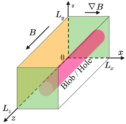
Although we are able to provide an arbitrary spatial profile for an external magnetic fieldBin the p3bd code, it is assumed thatBis parallel to thezdirection as shown in Fig. 1 and that the strength ofBis set as
B(x)= 2LxBLx 3Lx−x
, (6)
that is,∂B/∂x>0, in this study. Here,Lx,Ly, andLzare the system size in thex,y, andzdirections andBLxis the magnetic field strength atx = Lx. Thus, the−x,y, andz directions correspond to the radial, poloidal, and toroidal
Fig. 1 Schematic diagram of the simulation configuration. The simulation system reproduces the boundary layer of mag-netic confinement devices.
directions, respectively.
On the boundaries atx=0 (corresponding to the ves-sel wall) and both edges in thezdirection (corresponding to the end plates) displayed as shaded plates in Fig. 1, plasma particles are absorbed and the electric potential is fixed as ϕ= 0. In the simulations, the sheath potential is formed self-consistently near edges in thezdirection without any artificial methods (e.g., a logical sheath) since the grid size satisfiesΔg=λD, whereλDis the Debye length. Some low energy electrons are reflected by the sheath potential and it is observed that the net current to the sheath is nearly equal to zero outside of the blob or the hole region. (In the higher or lower potential side in the blob or the hole region, the net current in thezdirection becomes∼encs[5], wherenand cs are the plasma density and the ion acoustic speed.) On the other hand, a periodic boundary condition is applied in theydirection. On the plane atx = Lx, plasma particles are reflected and the electric potential satisfies∂ϕ/∂x=0.
A blob or a hole is initially provided as a cylindrical form elongated between both edges in thezdirection. That is, the electron and ion particles in a blob and in back-ground plasma are initially distributed by
ns,init(x, y)=nsf0
1+nˆb0gx(x)gy(y)
, (7)
or the electron and ion particles in a hole and in back-ground plasma are initially distributed by
ns,init(x, y)=nsf0
1−nˆb0gx(x)gy(y)
, (8)
where nsf0 is the initial density of background plasma which satisfies
s
qsnsf0=0, (9)
ˆ
nb0is the ratio between the initial density amplitude of the blob or the hole and background plasma density,gxandgy are defined by
gx(x)=exp
⎛
⎜⎜⎜⎜⎝−(x−xb0)2 2δ2
bx
⎞
⎟⎟⎟⎟⎠, (10)
and
gy(y)=exp
⎛ ⎜⎜⎜⎜⎜
⎝−(y−yb0)
2
2δ2 by
⎞ ⎟⎟⎟⎟⎟
⎠, (11)
respectively. (xb0, yb0) is the initial position of the center of a blob or a hole, andδbxandδbyare the blob or hole widths in thexandydirections. Equations (7), (8), (10), and (11) show that the blob or the hole is initially located along the ambient magnetic field around (xb0, yb0).
functions, where the 1D cumulative distribution functions are given by
Gbx(x)=
x
0
gx( ˜x) d ˜x
Lx
0
gx( ˜x) d ˜x
, (12)
and
Gby(y)=
y
0
gy(˜y) d ˜y
Ly
0
gy(˜y) d ˜y
. (13)
In the hole case, we cannot apply the same method as that in the blob case, i.e., using the 1D cumulative dis-tribution functions, because the density profiles as a dug hole cannot be given by superimposing the inversions of the 1D cumulative distribution functions. Thus, we have developed a new method which uses the two-dimensional (2D) cumulative distribution function. The initial density equation, Eq. (8), is separated into
ns,init1=nsf0(1−nˆb0), (14) and
ns,init2(x, y)=nsf0nˆb0
1−gx(x)gy(y)
. (15)
The code first distributes the particles of the first part de-scribed by Eq. (14) uniformly in the 3D space by using random numbers. Secondly, the particles of the second part described by Eq. (15) are distributed by using random numbers and the inversion of the 2D cumulative distribu-tion funcdistribu-tion, where the 2D cumulative distribudistribu-tion func-tion is given by
Gh(x, y)=
y
0
x
0
[1−gx( ˜x)gy(˜y)] d ˜xd˜y
Ly
0
Lx
0
[1−gx( ˜x)gy( ˜y)] d ˜xd ˜y . (16)
Actually, the code calculates the 2D cumulative distribu-tion funcdistribu-tion by
Gh(i)= i
j=1
[1−gx( ˜xj)gy( ˜yj)]ΔxΔy MxMy
j=1
[1−gx( ˜xj)gy(˜yj)]ΔxΔy
, (17)
where
xj= Δx[j−Mxint(j/Mx)−0.5], (18) yj= Δy[int(j/Mx)+0.5], (19) iand j are integer numbers, andMxand My are also the integer numbers defined byMx=Lx/ΔxandMy=Ly/Δy. Since Eqs. (17)–(19) provide the discrete positions in the ydirection to particles, the positions in theydirection are obtained from the discrete positions given by Eqs. (17)– (19) by the linear interpolation and random numbers.
The simulation system of the p3bd code does not have
particle and heat sources. Although the density distribu-tion does not satisfy equilibrium with the magnetic field as seen in Eqs. (6), (7), and (8) and the temporal evolution of the magnetic field is not solved, as mentioned above, such assumptions are appropriate in the low beta limit.
3. Blob and Hole Dynamics
We now consider the theoretical estimation of blob and hole propagation dynamics on the basis of the simple fluid model. The blob and hole dynamics are described by the equation for the charge conservation [1],
∇⊥·j⊥+∇j=0, (20)
where j⊥andjare the currents perpendicular and parallel to the magnetic field. The perpendicular current, j⊥, in-cludes the currents caused by the polarization and grad-B drifts, i.e.,
j⊥= jp+jg, (21)
where the polarization drift current and the grad-B drift current are given by
jp=−
⎛ ⎜⎜⎜⎜⎜ ⎝
s nsms
⎞ ⎟⎟⎟⎟⎟ ⎠B12
D(∇⊥φ)
Dt , (22)
and
jg=
⎛ ⎜⎜⎜⎜⎜ ⎝
s nsTs
⎞ ⎟⎟⎟⎟⎟ ⎠B12
∂B ∂x
y
y, (23)
respectively. Here, D/Dtrepresents the Lagrangian deriva-tive defined by∂/∂t+uE×B·∇,uE×Bis theE×Bdrift veloc-ity,Tsis the initial temperature, and we assume that Bis parallel to thezdirection and thatB(=|B|) depends upon onlyx.
3.1
Sheath-limited case
In the case where the parallel current, j, is limited by the sheath formed on the end plates, the divergence of the parallel current is given by the following equation [11],
∇j= j,Lz− j,0 Lz
=2 j,Lz Lz = 2 Lz ⎡ ⎢⎢⎢⎢⎢ ⎣ s
qsns,Lzvzs,Lz
⎤ ⎥⎥⎥⎥⎥ ⎦
=2neme csi Lz ⎡ ⎢⎢⎢⎢⎢ ⎣ ⎛ ⎜⎜⎜⎜⎜ ⎝ l nlm nem ql e csl csi
csl = (Te/ml)1/2, φ is the electric potential in the main plasma, and the subscripts e, i, andl represent the elec-tron, the major ion, and a species of ions (including the major ion), respectively. In the derivation of Eq. (24), we assume thatqe = −e and use the relations, nl,Lz = nlm, vzl,Lz = csl(1+Tl/Te)1/2, ne,Lz = nemexp(−eφ/Te), and vze,Lz=vTe/
√
2π, wherevTsis the initial thermal velocity. Using Eqs. (22)–(24) and assuming that D/Dt=0 and thatnlm=nem(nlf0/nef0), Eq. (20) becomes
csi
⎛ ⎜⎜⎜⎜⎜ ⎝1+
l nlf0 nef0 Tl Te ⎞ ⎟⎟⎟⎟⎟ ⎠mB2i
∂B ∂x
∂(lnnem) ∂y
+2e Lz ⎡ ⎢⎢⎢⎢⎢ ⎣ ⎛ ⎜⎜⎜⎜⎜ ⎝ l nlf0 nef0 ql e csl csi
1+Tl Te ⎞ ⎟⎟⎟⎟⎟ ⎠ − mi 2πme exp −eφ Te
=0, (25)
wherensmis substituted fornsin Eq. (23). Since the prop-agation speed of a blob or a hole is given by thex compo-nent ofuE×B, that is,−(∂φ/∂y)/B, the derivative of Eq. (25) regardingyprovides the propagation speedvbas
vb csi =
1 2AshLzρ
2 si B2 Lx B3 ∂B ∂x
∂2(lnn em)
∂y2 , (26)
whereAshandρsiare defined by Ash=
q2i e2
⎛ ⎜⎜⎜⎜⎜ ⎝1+
l nlf0 nef0 Tl Te ⎞ ⎟⎟⎟⎟⎟ ⎠ 2πme mi exp eφ Te , (27)
andρsi =csi/Ωi, respectively, andΩiis the cyclotron fre-quency of the major ion atx=Lx.
Substituting Eqs. (6) and (7) forBandnemin Eq. (26), respectively, we obtainvbin this study as
vb csi =−
AshLz 8Lx
3− x Lx
1− nef0 ne,init(x, y)
×
⎡ ⎢⎢⎢⎢⎢
⎣1− nef0 ne,init(x, y)
(y−yb0)2 δ2 by ⎤ ⎥⎥⎥⎥⎥ ⎦ ρ 2 si δ2 by . (28)
(Even if we substitute Eq. (8) fornem, Eq. (28) is derived. That is,vbfor the hole case is given by the same equation as that for the blob case.) Equation (28) indicates that a blob or a hole propagates in the∓∇B direction and that the propagation speed is proportional toδ−2by. Furthermore, it is obvious that the shear term in Eq. (28), i.e., the term including (y−yb0)2, will become larger in the hole case than the shear term in the blob case because ˆnb0<1 in the hole case although ˆnb0is not restricted in the blob case [6].
3.2
Periodic boundary case
In this section, we now consider the case without the end plates, that is, with the periodic boundary condition applied in thezdirection. This situation is called the “in-ertial” case in previous papers [1] because the dynamics are determined by the inertial term in the model equation rather than by the sheath term. In this case, the divergence of the parallel current is given by
∇j=0, (29)
with the assumption that the dynamics are independent of z. Therefore, Eq. (20) becomes
B
B·
D
Dt(∇⊥×uE×B)
=Aprc2si ∂(lnB)
∂x
∂(lnne) ∂y , (30) where the Boussinesq approximation is used. It is assumed thatnl=ne(nlf0/nef0).Apris defined by
Apr=
1+ l nlf0 nef0 Tl Te s nsf0 nef0 ms mi . (31)
Furthermore, we use the electron continuity equation, Dne
Dt =−uge·∇⊥ne−ne∇⊥·(uE×B+uge) = Te
eB2 ∂B ∂x
∂ne
∂y −ne∇⊥·uE×B, (32) whereugeis the electron grad-Bdrift velocity. Linearizing Eqs. (30) and (32), we obtain the estimation of the blob or hole propagation speed [1, 12] as
vb≈csi
Apr δbx B ∂B ∂x
1/2
. (33)
In the derivation of Eq. (33), theycomponent ofuE×Band the wave number in theydirection, ky ∼ 1/δby, are ne-glected.
4. Simulation Results
We next show simulation results calculated by the p3bd code. In this section, results of blob and hole propa-gation simulations in both the sheath-limited and periodic boundary cases are presented and compared with the theo-retical estimations.
Table 1 Parameters of blob propagation simulations.
Symbol (Sheath/Periodic) Δg/ρsi ΩiΔt δbx/ρsi δby/ρsi
•/◦ 0.488 1.22×10⁻³ 1.95 1.46
/ 0.484 1.21×10⁻³ 1.94 1.94
/ 0.477 1.19×10⁻³ 1.91 2.86
/ 0.470 1.17×10⁻³ 1.88 3.76
/♦ 0.457 1.14×10⁻³ 1.83 5.48
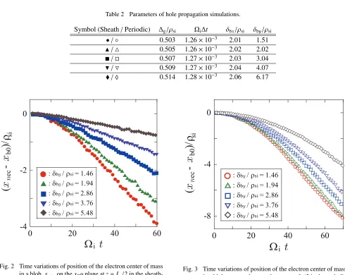
Table 2 Parameters of hole propagation simulations.
Symbol (Sheath/Periodic) Δg/ρsi ΩiΔt δbx/ρsi δby/ρsi
•/◦ 0.503 1.26×10⁻³ 2.01 1.51
/ 0.505 1.26×10⁻³ 2.02 2.02
/ 0.507 1.27×10⁻³ 2.03 3.04
/ 0.509 1.27×10⁻³ 2.04 4.07
/♦ 0.514 1.28×10⁻³ 2.06 6.17
Fig. 2 Time variations of position of the electron center of mass in a blob,xnec, on thex–yplane atz=Lz/2 in the
sheath-limited case. The circles (•), triangles (), squares (), inverse triangles (), and diamonds () represent results of calculations shown in Table 1, respectively.
initial background plasma. The initial density ratio of the blob to the background plasmas is ˆnb0 = 2.7 in the blob case. On the other hand, the initial density ratio between the center of the hole and the background plasma is set as 1−nˆb0 =0.27 in the hole case. The initial blob width or hole width in the radial direction isδbx=4Δg ≈2ρsi. The initial poloidal width of a structure is given byδby/Δg=3, 4, 6, 8, or 12 as seen in Tables 1 and 2. The initial positions of the blob and the hole are (xb0, yb0)=(3Lx/4,Ly/2) and (Lx/2,Ly/2), respectively.
In Figs. 2 and 3, we show the results of blob
propaga-Fig. 3 Time variations of position of the electron center of mass in a blob,xnec, on thex–yplane atz=Lz/2 in the periodic
boundary case. The circles (◦), triangles (), squares (), inverse triangles (), and diamonds (♦) represent results of calculations shown in Table 1, respectively.
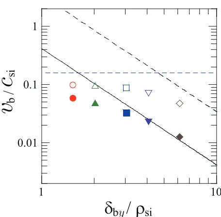
Fig. 4 Relation between the poloidal blob size,δby, and the blob radial propagation speed,vb. The solid and open symbols
represent the observed propagation speeds in the calcula-tions with the parameters shown in Table 1 in the sheath-limited and periodic boundary cases, respectively. The black solid and broken lines show the theoretical average and maximum speeds in the sheath-limited case. Also, the blue broken line presents the theoretical speed in the periodic boundary case.
in Fig. 3). We show the relation between the poloidal blob width,δby, and the blob propagation speed in the ra-dial direction,vb, in Fig. 4. In this figure, the black lines and the blue broken line represent the theoretical speeds in the sheath-limited and periodic boundary cases given by Eqs. (28) and (33), respectively. In the computation of these theoretical speeds, we use the initial parameters shown above and assume that the potential inAshdescribed by Eq. (27) is given by
eφ Te =
1 2 ln
mi 2πme(1+Ti/Te)
, (34)
which is obtained from the condition in which the net cur-rent to the sheath is zero, that is,ne,Lzvze,Lz=ni,Lzvzi,Lz. The black solid line designates the average speed and the black broken line designates the maximum speed, where the av-erage speeds are calculated by
vb=
σvb(x, y)gx(x)gy(y) dxdy σgx(x)gy(y) dxdy
, (35)
σis the area defined by (x−xb0)2
2δ2 bx
+(y−yb0)2 2δ2
by
ln(10), (36)
and the maximum speeds are obtained by substituting (xb0, yb0) for (x, y) in Eq. (28).
Fig. 5 Time variations of position of the electron center of mass in a hole,xnec, on thex–yplane atz=Lz/2 in the
sheath-limited case. The circles (•), triangles (), squares (), inverse triangles (), and diamonds () represent results of calculations shown in Table 2, respectively.
Fig. 6 Time variations of position of the electron center of mass in a hole,xnec, on thex–yplane atz=Lz/2 in the periodic
boundary case. The circles (◦), triangles (), squares (), inverse triangles (), and diamonds (♦) represent results of calculations shown in Table 2, respectively.
Fig. 7 Relation between the poloidal hole size,δby, and the hole radial propagation speed,vb. The solid and open symbols
represent the observed propagation speeds in the calcula-tions with the parameters shown in Table 2 in the sheath-limited and periodic boundary cases, respectively. The black solid and broken lines show the theoretical average and maximum speeds in the sheath-limited case. Also, the blue broken line presents the theoretical speed in the periodic boundary case.
xnec=
H
x[nef(1−nˆb0/10)−ne(x, y)] dxdy
H
[nef(1−nˆb0/10)−ne(x, y)] dxdy ,
(37) where H is the area in which the electron density, ne, is lower thannef(1−nˆb0/10) andnefis calculated by the same process as that mentioned above. Also, we obtain the hole propagation speeds in each simulation from the data ofxnec betweenΩit = 20 and 60 (the sheath-limited case shown in Fig. 5) orΩit =40 and 70 (the periodic boundary case shown in Fig. 6). Figure 7 shows the relation between the poloidal hole width, δby, and the hole propagation speed in the radial direction, vb. The black lines and the blue broken line in this figure represent the theoretical speeds in the sheath-limited and periodic boundary cases given by Eqs. (28) and (33), respectively. In the computation of these theoretical speeds, we use the initial parameters shown above and assume that the potential inAshdescribed by Eq. (27) is given by Eq. (34). The black solid line ignates the average speed and the black broken line des-ignates the maximum speed, where the average and maxi-mum speeds are obtained by the same calculations as those shown above.
Figures 4 and 7 indicate that the observed propagation speeds are in agreement with the theoretical estimation. In the sheath-limited case, the observed propagation speeds
of small blobs and holes are slower than the theoretical es-timation, which is thought to arise from kinetic effects be-cause of the approach of structure size to the ion Larmor ra-dius or from some instabilities because the poloidal width δbyof such blobs is smaller thanδ∗∼ρsi[Lz2/(ρsiLx)]1/5, whereδ∗is the particular width for the long distance propa-gation as shown by Eq. (17) in Ref. [1] andδ∗∼3ρsiin this study. (In these sheath-limited case simulations, dynam-ics by instabilities [e.g., the evolution to mushroom shape] are not observed clearly because the calculation time is too short to observe such dynamics due to the smallLz.)
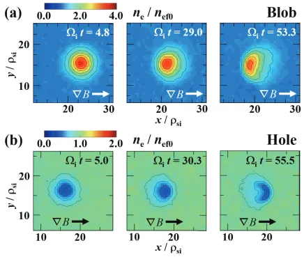
Figure 8 shows the time evolutions of the electron den-sity distribution on thex–yplane atz = Lz/2 in the blob (a) and hole (b) propagations in the sheath-limited case. This figure indicates that the distortion of the hole shape is larger than that of the blob shape. The large distortion of the hole shape occurs by the velocity shear as mentioned in Sec. 3.1.
5. Summary and Discussion
We have developed, updated, and verified the electro-static 3D-PIC simulation code for the study of blob and hole propagation dynamics, that is, the p3bd code. We are able to simulate the boundary layer plasma of magnetic confinement devices by the p3bd code. Although only a blob structure is initially provided in the simulation sys-tems in the previous version of the p3bd code, the updated p3bd code is able to simulate the hole propagation. For the verification of the code, we have estimated the theo-retical blob and hole propagation speeds and compared the observed blob and hole propagation speeds in the simula-tions with the theoretical estimasimula-tions. The observed rela-tions between the propagation speed and the structure size in both the blob and the hole cases are in good agreement with the theoretical relations. Also, the code has repro-duced the large distortion of the hole shape by the velocity shear.
Fig. 8 Time evolutions of the electron density distribution on thex–yplane atz=Lz/2 in the blob (a) and hole (b) propagations in the
sheath-limited case, whereδby/Δg=4. These simulations are represented by the triangle () in the above tables and figures.
layer during the detached state was observed in some ex-periments [18–21]. Although the electric field in a blob or a hole, namely, the radial propagation speed, is reduced by the short-circuit on the end plate in the attached state, the detached plasma might prevent the short-circuit. Actually, the simulations in this study show that the radial propa-gation speed of a blob or a hole without the short-circuit, i.e., in the periodic boundary case, is faster than that with the short-circuit, i.e., in the sheath-limited case, as seen in Figs. 4 and 7.
Acknowledgments
The simulations were carried out on the Plasma Simulator (PS) of the National Institute for Fusion Sci-ence (NIFS) and the high-performance computer sys-tem of Nagoya University. This work is performed with the support and under the auspices of the NIFS Collaboration Research programs (NIFS15KNSS058, NIFS14KNXN279, NIFS15KNTS039, NIFS15KNTS040, and NIFS16KNTT038), supported by a Grant-in-Aid for Scientific Research from the Japan Society for the Pro-motion of Science (KAKENHI 23740411), and partially
supported by “Joint Usage/Research Center for Inter-disciplinary Large-scale Information Infrastructures” and “High Performance Computing Infrastructure” in Japan (jh160023-NAH).
[1] S.I. Krasheninnikov, D.A. D’Ippolito and J.R. Myra, J. Plasma Phys.74, 679 (2008) and references therein. [2] D.A. D’Ippolito, J.R. Myra and S.J. Zweben, Phys. Plasmas
18, 060501 (2011) and references therein.
[3] S. Ishiguro and H. Hasegawa, J. Plasma Phys. 72, 1233 (2006).
[4] H. Hasegawa and S. Ishiguro, Plasma Fusion Res. 7, 2401060 (2012).
[5] H. Hasegawa and S. Ishiguro, Phys. Plasmas22, 102113 (2015).
[6] S.I. Krasheninnikovet al., Proc. 19th IAEA Fusion Energy Conf. (Lyon, France, 2002) (International Atomic Energy Agency, Vienna, 2003) IAEA-CN-94/TH/4-1.
[7] H. Hasegawa and S. Ishiguro, Proc. 26th IAEA Fusion ergy Conf. (Kyoto, Japan, 2016) (International Atomic En-ergy Agency, Vienna, 2017) IAEA-CN-234-0135/TH/ P6-17.
[9] C.K. Birdsall and A.B. Langdon, Plasma Physics via
Computer Simulation(McGraw-Hill Book Company, New
York, 1985, Institute of Physics Publishing, Bristol and Philadelphia, 1991, and Adam Hilger, Bristol and New York, 1991).
[10] W.H. Presset al.,Numerical recipes in Fortran 77 : The
art of scientific computing, 2nd ed.(Cambridge University
Press, New York, 1996).
[11] D.A. D’Ippolito, J.R. Myra and S.I. Krasheninnikov, Phys. Plasmas9, 222 (2002).
[12] J.R. Myra and D.A. D’Ippolito, Phys. Plasmas12, 092511 (2005).
[13] D. Jovanovi´c, P.K. Shukla and F. Pegoraro, Phys. Plasmas
15, 112305 (2008).
[14] J.D. Angus, S.I. Krasheninnikov and M.V. Umansky, Phys. Plasmas19, 082312 (2012).
[15] T. Takizuka and H. Abe, J. Comput. Phys.25, 205 (1977). [16] K. Nanbu, Phys. Rev. E55, 4642 (1997).
[17] T. Pianpanit, S. Ishiguro and H. Hasegawa, Plasma Fusion Res.11, 2403040 (2016).
[18] R. Décosteet al., Plasma Phys. Control. Fusion38, A121 (1996).
[19] B.L. Stansfieldet al., J. Nucl. Mater.241-243, 739 (1997). [20] N. Ohno, K. Furuta and S. Takamura, J. Plasma Fusion Res.
80, 275 (2004).