Multiple Tabu Search for Multiobjective Urban Transit
Scheduling Problem
Vikneswary Uvaraja1, Lai Soon Lee 1,2,*, and Nor Aliza Ab. Rahmin1
1 Department of Mathematics, Faculty of Science, Universiti Putra Malaysia, 43400
UPM Serdang, Selangor, Malaysia.
2Laboratory Computational Statistics and Operations Research, Institute for
Mathematical Research, Universiti Putra Malaysia, 43400 UPM Serdang, Selangor, Malaysia.
∗Corresponding author: [email protected]
The study of urban public transportation is essential for building an efficient transit system that can minimize the traffic congestion, reduce pollutions and increase the mobility of a community. Urban Transit Scheduling Problem (UTSP) considers the process of creating timely transit schedules that includes bus and drivers assignment based on the users’ and operators’ requirements. It is necessary to achieve a tradeoff between the interest of users and operators which lead to multiobjective nature of UTSP. This paper studies multiobjective UTSP consisting of frequency setting, timetabling, simultaneous bus and driver scheduling by applying a Multiple Tabu Search (MTS) algorithm. In addition, a multiobjective set covering model is also adapted by including some real-world restrictions to find adequate number of buses and drivers. The MTS algorithm is tested on benchmark instances from Mandl’s Swiss Network. The computational results shown that the algorithm able to produce comparable results for most cases from the literature.
Keywords: Urban Transit, Scheduling, Multiobjective, Tabu Search.
I.
Introduction
The development of urban public transit tech-nology has major impact on the size of a city and its population and vice versa. The lack of systematic public transportation system will always lead to various conflicts such as traffic congestion and air pollution. Nevertheless, it is often difficult to improve the public transport system since many criteria need to be taken into consideration which includes passenger’s
and operator’s preferences. It is necessary
to include both of their perspectives in order to increase the ridership with minimal use of resources. Some of the major disadvantages of urban public transportation are longer waiting time and its non-availability to destination at desired time.
This type of problem can be classified as Urban Transit Scheduling Problem (UTSP) which involves the process of deriving optimal schedules for buses and drivers with respect to the passenger’s demand and operator cost. UTSP can be divided into frequency setting,
timetabling, vehicle and crew scheduling
(Ceder, 2002). Generally, these problems are tackled consecutively due to its complexity. UTSP is a complex NP-hard problem and many approaches have included mathematical models to formulate the problem and solve
it quantitatively through optimization.
Re-cently, researchers are turning to the study of multiobjective UTSP which is related to
the interaction of passengers’ preferences
and the industry regulation to provide more
choices for decision makers. The process of
of both stakeholders is quite difficult as it depends on the requirement of decision makers.
Metaheuristic have been a popular method for solving this hard combinatorial optimiza-tion problem due to its capability of finding near optimal solutions in reasonable time
(Nikoli´c and Teodorovi´c, 2014). However,
there is no such application of Multiple Tabu Search (MTS) in multiobjective UTSP are known to date. Thus, MTS with systematic neighborhood selection approach is developed by modifying the initialization process and
incorporating intensification and
diversifi-cation to find optimal solutions for solving multiobjective UTSP. The proposed algorithm is verified and validated using benchmark data sets to generate competitive solutions with previously published results.
In this study, a multiobjective mixed integer programming model that the minimize number of buses, total waiting times and overcrowding is formulated to find suitable frequency for each of the routes studied. The model is further ex-tended including timeslots to set the frequen-cies during peak and off-peak hours throughout the time period. On the other hand, a set cov-ering model is adapted from Zuo et al. (2015) to minimize the number of buses and drivers simultaneously for constructing optimal sched-ules.
Over the years, UTSP has been solved by different approaches based on the problem’s complexity and the development of computer
technology. At the early stage, researchers
have tackled only the frequency or headways optimization problem. Beginning from 1976, timetabling problem has been introduced to produce efficient schedules and followed by vehicle and crew scheduling approach. Due to the scope of this paper, only the application of TS in UTSP is dicussed in this section.
Cavique et al. (1999) discussed two heuris-tic approaches for crew scheduling problem to minimize the crews required to cover a
predefined timetable under contractual rules. The first algorithm uses strategic oscillation
procedure and the second applied block
partitions and matching algorithm in Tabu subgraph ejection chain where the latter gives
better performance. Gomes et al. (2006)
extended it to balance the number of drivers and cover crews since the non-driving periods
are usually longer than total duty time. A
Lisbon Underground case study is used to test effectiveness of the TS algorithm.
The first study to consider multiobjective bus driver scheduling problem based on TS and Genetic Algorithm (GA) is Louren¸co et al. (2001). A TS with three types of neighbour-hood selection and optimized intensification strategy is applied to find the best solutions. Based on the results, the TS outperformed the other methods as linear programming in
term of cost, time and quality. Moreover,
Ruisanchez and Ibeas (2012) constructed a bi-level optimization model to assign optimal bus sizes and frequencies to public transport
routes. The upper level problem minimizes
the cost of users and operators while the lower level model solved public transport assignment
model subject to capacity constraint. The
basic TS algorithm can converge quickly to optimal solution than Hooke-Jeeves algorithm (HJ) when compared using real-world problem. Similarly, Giesen et al. (2016) also proposed a TS algorithm combined with aspiration plus strategy for solving multiobjective transit frequency optimization. The objectives are to minimize the total travel time and operator
cost. The proposed algorithm improved the
current solution in term of total travel time and fleet size.
for benchmark data sets. Finally, Section 5 presents conclusion and suggestions for future research.
II.
Multiobjective Urban
Transit Scheduling
Problem
UTSP is a multiobjective problem in nature as it must considers the preferences of both users and operators which are always conflicting to each other. Passengers would choose to travel quickly from their origin to destination with shorter waiting time and high comfort. On the contrary, operators would try to minimize their operational cost in term of the number of buses and drivers required which consequently might
reduce the quality of service. This problem
can be solved either by setting weights to the objectives according to its relative importance to obtain a single solution or handling them simultaneously to produce various solutions with different tradeoff levels.
Many models combine these objectives into single function under the resources constraints such as fleet size (Scheele, 1980; Constantin and Florian, 1995) and bus loading (Verbas and Mahmassani, 2015; Li et al., 2013). As for the second case, an optimal solution is chosen from the set of non-dominated solutions which can also be obtain by executing the single objective model consecutively using different weights of the objectives and constraints values. On the other hand, the studies on multiobjective op-timization to produce Pareto optimal solutions in a single execution are increasing in order to explore different range of solutions and observe the relation between the objectives for long-term planning (Fedorko and Weiszer, 2012; Zuo et al., 2015; Prata, 2016).
A. Frequency Optimization
The frequency optimization problem can be formulated as a bilevel procedure to show the interaction between transit users and
operators. Initially, the frequency is assigned based on the available resources and the users planned their travel according to the
service design. Then, the transit operator
improved the service frequency by observing the users’ travel pattern. The first procedure describes about passenger assignment method that represents their route choice behaviour based on the Mandl’s transportation network design which includes fixed demand and deterministic travel times for both direction of an origin-destination (OD) pair. The second stage discusses the frequency optimization pro-cedure by MTS. The optimal set of frequency is used to update the initial frequency and the procedure is reiterated until convergence pattern of the frequency set is observed.
In this study, two cases are considered to find the optimal frequency for each route. The first case assumed that the demand and frequency of a route are constant throughout the time period studied whereas for the second case, the problem is extended to vary the demands between each OD pair and frequencies of the routes according to specific timeslot. The no-tations to represent the passenger assignment and frequency optimization models are shown below.
Two passenger assignment methods are adopted from Baaj and Mahmassani (1991)
and Afandizadeh et al. (2013). Generally, a
passenger can use at most two transfers to travel between their OD pair. It is expected that the passenger will first select a direct path without any transfer to reach their destination. When no direct path is available, the passengers prefer to travel by one transfer. If there is no one transfer path provided for the OD pair, the path with two transfers is chosen. The demand is usually considered unsatisfied when more than two transfers are needed for
travelling. The difference between the two
dij number of passengers travelling between nodesiandj
dij,s number of passengers travelling between nodesiandj
in timeslots
fk frequency of routek
fk,s frequency of routekin timeslots
fmin minimum frequency for a time period fmax maximum frequency for a time period lk layover time of routek
Qk maximum load (passengers) of routek
Qk,s maximum load (passengers) of routekin timeslots
tpi,j total travel time of a passenger between nodesiandj
on pathp
tpi,j,s total travel time of a passenger between nodesiandj on pathpin timeslots
tpinvt,ab in-vehicle travel time between nodesaandbfor path
p
tpwt,a waiting time of a passenger at nodeafor pathp tptt,b transfer time (penalty per transfer) of a passenger at
nodebfor pathp
tpinvt,ab,s in-vehicle travel time between nodesaandbin timeslotsfor pathp
tpwt,a,s waiting time of a passenger in timeslotsat nodea for pathp
tptt,b,s transfer time (penalty per transfer) of a passenger in timeslotsat nodebfor pathp
tk vehicle travel time of routek
up utility function represent the probability for each of the pathpto be chosen
CAP seating capacity of a bus DWP dwell time for a passenger LF load factor of a bus R set of bus routes
Rab set of potential routes between nodeaandb
T time horizon TS set of timeslots
N set of nodes in transit network
Based on Baaj and Mahmassani (1991), when direct paths are available between OD pair, the in-vehicle travel time of each route is computed and a filtering process is invoked such that any route with in-vehicle travel time more than 50% (or a pre-specified threshold) of the minimum value is rejected.Then, the demands are distributed to the surviving routes using ‘frequency share’ rule: a route carries a part of the flow equal to the ratio of its frequency to the sum of the frequencies of all acceptable routes.
If multiple one transfer or two transfer routes are found, the total travel time of a passenger at each possible path that sum up the in-vehicle travel time, waiting time and
transfer time between origin,iand destination,
j is calculated. Equations (1) and (2) find
the total travel time for one and two transfers respectively. The passenger’s waiting time at the origin and transfer node are assumed to be
half of the headway of a routek. The transfer
nodes are defined asnandn0 in the equations.
Next, a filtering procedure similar to the zero-transfer is applied such that all paths whose total travel time are higher than 10% (or a pre-specified threshold) of the minimum value offered by any paths between that pair of nodes are rejected. The detail explanation of this passenger assignment process is stated
in Nikoli´c and Teodorovi´c (2014).
Based on Afandizadeh et al. (2013), if multi-ple direct paths exist, each path has a possibil-ity to be chosen based on its route frequency. Frequency share rule is applied to allocate the demands based on the respective frequency of each route on the chosen paths. Alternatively, the passengers are assigned according to the to-tal travel time utility in case there are multiple paths exist with one or two transfers from the origin to destination. The travel time utility is calculated from the formula of Logit model as shown in equation (3) where the total travel time is equal to equation (1) or (2) according to the number of transfer.
tpi,j=tpinvt,ij+tpwt,ij+tptt,ij,
= [tpinvt,in+tpinvt,nj] + [tpwt,i+tpwt,n] +tptt,n,
= [tpinvt,in+tpinvt,nj] + [( T 2P
k∈Rinfk
)p (1)
+ ( T
2P k∈Rnjfk
)p] +tp tt,n.
tpi,j=tpinvt,ij+tpwt,ij+tptt,ij,
= [tpinvt,in+tp
invt,nn0 +t p invt,n0j]
+ [tpwt,i+tpwt,n+t p wt,n0] + [t
p tt,n+t
p tt,n0],
= [tpinvt,in+tp
invt,nn0 +t p
invt,n0j] (2)
+ [( T 2P
k∈Rinfk
)p+ ( T
2P k∈R
nn0
fk
)p
+ ( T
2P k∈R
n0j
fk
)p] + [tptt,n+tp
up=
e−(t
p ij)
P p∈Pe−(t
p ij)
. (3)
This procedure is extended by including timeslots in order to differentiate peak and
off-peak hours. During the assignment process,
the passengers are allocated based on the fre-quencies of the routes at that time period. First, the frequencies of the routes and the de-mand for every OD pair are divided propor-tionally according to peak and off-peak hours. The demands on the peak hours are assumed to be double the demands on off-peak hours.The total travel time of a passenger at each times-lot for every possible path from their origin to destination is calculated. Likewise, equations (4) and (5) are applied to find the total travel time of the path with one and two transfers respectively.
tpi,j,s=tpinvt,ij,s+tpwt,ij,s+tptt,ij,s,
= [tpinvt,in,s+tpinvt,nj,s] + [tpwt,i,s+tpwt,n,s]
+tptt,n,s,
= [tpinvt,in,s+tpinvt,nj,s] + [( T 2P
k∈Rinfk,s
)p (4)
+ ( T
2P
k∈Rnjfk,s
)p] +tptt,n,s.
tpi,j,s=tpinvt,ij,s+tpwt,ij,s+tptt,ij,s,
= [tpinvt,in,s+tp
invt,nn0,s+t p invt,n0j,s]
+ [tpwt,i,s+tpwt,n,s+tp
wt,n0,s]
+ [tptt,n,s+tp
tt,n0,s],
= [tpinvt,in,s+tp
invt,nn0,s+t p
invt,n0j,s] (5)
+ [( T 2P
k∈Rinfk,s
)p+ ( T 2P
k∈R
nn0
fk,s
)p
+ ( T
2P k∈R
n0j
fk,s
)p] + [tp tt,n,s+t
p tt,n0,s].
All routes are initialized with similar fre-quency before the passenger’s demand is
assigned based on the route choice. After
the passenger assignment process, the
max-imum load of each route k is obtained from
its list of link flows and used as the input for the frequency optimization procedure. The objectives are the minimization of total number of buses, passengers waiting time and
overcrowding in the bus. Most of the papers in the literature have used these objectives
for optimizing the frequency. The passenger
assignment procedure is conducted to find the total waiting time of all passengers.
minimize
F1=
X k∈R
[2tkfk
T ], (6)
F2=
X
i∈N X
j∈N
[dij
T
2Pk∈R
ijfk
], (7)
F3=
X k∈R
[Qk−(CAP(LF)fk)], (8)
subject to
fmin≤fk≤fmax for all k∈R. (9)
Equation (6) calculates the number of buses needed for each route that obtained by dividing the total round trip time with the time horizon. Equation (7) measures the total waiting time for all the passengers. Equation (8) determines the total number of passengers that exceed the maximum capacity of the bus. Equation (9) ensures that frequency of each route is within the lower and upper boundary
value. Consequently, the previous model is
further extended by incorporating timeslots in order to find the frequency of a route in a specific time period based on the variable demands as follows:
minimize
F1=
X k∈R
[maxs∈T S(
2tkfk,s+Qk,sDW P+lkfk,s
T )],
(10)
F2=
X i∈N
X j∈N
X s∈T S
[dijs
T
2P
k∈Rijfk,s
], (11)
F3=
X k∈R
X s∈T S
[Qk,s−(CAP(LF)fk,s)], (12)
subject to
fmin≤fk≤fmax for all k∈R. (13)
Equation (10) determines the maximum number of buses needed among all the timeslots for each route. The round trip time includes
measures the total waiting time for all the pas-sengers in every timeslot while equation (12) calculates the total number of passengers that exceed the maximum capacity of the bus in all timeslots. Equation (13) shows the constraint on the frequency of each route.
B. Bus and Driver Scheduling
The proposed procedure for solving these prob-lems is inspired from Zuo et al. (2015) who tackled the vehicle scheduling problem. The solution approach is revised by incorporating the elements for bus driver scheduling. It is assumed that the drivers are assigned to the same bus throughout their working time to en-sure systematic assignment process. A driver is assigned to the departure times based on sev-eral work load rules such as total work dura-tion, maximum working period without break and maximum break duration which are set as follows with its value in the bracket:
Dbreak: maximum break duration (1 hour),
Dwork: maximum working duration without
break (4 hours),
Dwork: total work duration (9 hours).
Each route has two control points (CP1 and
CP2) which represent the first and last nodes
of the route at where the drivers can take a break for a specific duration. There are two scenarios considered in this study for solving bus and driver scheduling problem. The first scenario favors passengers requirement by
assigning equal departure times to both CPs
while the second scenario consider operators
preference by allocating the time at CP1 only.
The solution procedure for both scenario is similar except the formation of blocks varies when choosing the departure times.
The scheduling process can be subdivided into three stages. Initially, a set of blocks is produced to cover all the departure times. Then a subset of candidate blocks is selected from them which minimize the objective
functions. Later, all the candidate blocks are reconstructed to further reduce the objective functions values. The process is repeated for
all the routes. Let Ak1 and Ak2 be the set of
departure time of the route k from both CP1
and CP2 respectively. The set of independent
blocks are grouped as Bk where q is the total
number of blocks and bky is the yth block of
Bk.
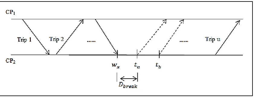
By referring to Figure 1, let trip 1 starts
from ax at CP1 and ends with wx at CP2.
For the first scenario, the departure time of
trip 2 will be tb which is the next available
time in the list of Ak2 after wx +Osk, where
Oks is the one-way travel times of route k
at timeslot s that includes layover time and
dwell time. Meanwhile, for the second case,
ta is the departure time for trip 2 such that
ta = wx +Oks. Note that, tb ≥ ta. The next
trip also continues to find the time in similar manner to complete the block. Moreover, the drivers break time also included in the block
after Dmaxb without considering the location.
Based on Figure 2, suppose wx is the
departure time after several trips and
wx−ax ≥Dmaxb, then the next trip must be
equal or higher thanwx+Dbreak. Likewise, tb
and ta are the succeeding trip for scenario 1
and 2 respectively. The maximum duration of a block is always checked before choosing the consequent trips. The construction of a block terminates if the departure time of the trip is
more than Dwork for a short block and 2Dwork
for a long block.
Figure 1: Construction of a Vehicle Block
Figure 2: Choosing Departure Times after Break
various combinations of trips for each bus. The set covering model for bus and driver scheduling is presented as follows:
minimize
Fl= q X y=1
zy, (14)
F2=
q X y=1
Cyzy, (15)
subject to
q X y=1
vxyzy≥1, (16)
zy={0,1} Cy={1,2} vxy={0,1} y= 1, ..., q.
where,
vxy=
1,if blockyhas a trip starting fromxth departure time
0,otherwise,
zy=
1,if block y is in the solution 0,otherwise,
zy=
1,ifbyis a short block
2,ifbyis a long block.
Equations (14) and (15) minimize the
number of buses and drivers respectively and equation (16) ensures that every departure
time is covered by at least one trip. vxy is
a binary matrix that records the availability of departure time in a block whereas the
binary decision variable zy shows the
pres-ence of blocks in the solution. The parameter
Cydefines the number of drivers for each block.
gener-ates extra vehicle blocks for the time that can-not be covered in the blocks created from initial departure times. This is because the adjust-ment of departure times may affect the head-way and layover time determined earlier which consequently have an impact on robustness of the schedule.
III.
Multiple Tabu Search
MTS has been first developed by Pothiya et al. (2006) to design the optimal fuzzy logic
proportional integral (PI) controller. The
conventional TS method might require longer computational time to find expected solution if the initial solution is further from the
promis-ing space. Thus, MTS algorithm highlights
the problem and helps to guide the search to the optimal region in less computational time.
MTS algorithm begins by generating several initial solutions to increase the possibility of
reaching the optimal region quickly. Then,
adaptive search mechanism is applied to alter the step size of the neighborhood accordingly during the search and multiple TS algorithms are performed sequentially according to its initial solution. Consequently, the new starting solutions for next iteration are obtained by crossover mechanism. The process is restarted when the search reached local optimal solution and stopped after the termination criterion is satisfied.
In this study, the proposed MTS algorithm functions distinctly for discrete optimization (bus and driver scheduling) and continuous optimization (frequency setting) problem. The performance of MTS is greatly depends on the initial solution as it affects the compu-tational time for the solution to converge. The proposed MTS algorithm works with multiple initial solutions such that each of them is selected from different feasible domain. Explicitly, the search space is divided into a number of domains and each of the domains is allocated to different range of values. This can
help to speed up the search and examine the search space precisely to find better solutions. We used variable precision value to create a flexible neighborhood structure since constant step size might not be able to move the
current solution efficiently. So, the adaptive
search mechanism is applied to find step sizes for locating the neighborhood of the current solution.
The use of single or multiple tabu lists depends on the types of move involved during the search that directly influenced by type of the problem. There are several elements added or dropped at the same time to create the neighborhood of current solution. Therefore, this study applied two-dimensional tabu lists with same tabu tenure to record the elements with their positions in the list. This approach inhibits repeated moves and enables the search to explore variety of solution using organized memory structure.
Moreover, intensification is executed if there is no promising solution available and diversifi-cation occurs when intensifidiversifi-cation is not possi-ble to be implemented. This is because the nor-mal search procedure in the proposed MTS is good enough to analyze a portion of the whole neighborhood since it is divided earlier. Addi-tionally, there is no need to spend extra time to examine the region that already visited pre-viously. On the other hand, aspiration criteria allows tabu moves if it yields the best results and termination criteria stop the search if there is no progress in the objective values after a fixed number of iterations.
A. MTS for Frequency
Optimization
Initially, the range of frequency for each route is
divided intom number of domains using
equa-tion (17) and the procedure to set the individ-ual range is explained as follows:
dif = fmax−fmin+ 1
Step 1: Let k= 1.
Step 2: Set f1,min=fmin and fm,max=fmax.
Find the intervaldif for the routek.
Step 3: Let n= 1, calculate fn,max
=fn,min+dif−1
andfn+1,min=fn,max+ 1.
Step 4: Repeat Step 3 untiln=m−1.
Step 5: Repeat Steps 2-4 for all route k∈R.
Each of the routes is assigned to the ran-dom frequencies within their boundaries. The initial solutions are represented as a vector of
X0
n=fn01,fn02,···,fmw0 , such that wis the number of
routes. The neighborhoods of the current solu-tions are formed by increasing and decreasing the frequencies based on the step size values which are obtained randomly by Equation (18). The step size reduces as the number of iteration increases. This approach can produce more ac-curate solution in minimal computational time.
Let40
n=40n1,4n02,···,40mw represents the vector of
step size for the multiple solutions.
40
n=K×rand()×(fn,max−fn,min). (18)
The weight factor, K is calculated as follows:
K=wmax−
wmax−wmin
itermax
×iter, (19)
where, rand() is a random value between the
interval (0,1], wmax is the maximum weight,
wmin is the minimum weight, itermax is the
maximum iteration and iter is the current
iteration. In this study, wmax=1.0, wmin=0.2
and itermax=100.
Each solution in the neighborhood is checked for its feasibility, tabu restriction and domi-nance respectively. It is kept in a set of non-dominated solutions if it satisfy all the crite-ria. The set is always updated by removing the worse solutions each time after a solution is added. Then, a new solution is randomly selected from the set to be assigned as next current solution. All other non-dominated so-lutions are stored in intermediate-term mem-ory for intensification. When there is no dom-inated solution available, intensification pro-cess is conducted by choosing a solution from
intermediate-term memory. Alternatively, if
the intermediate-term memory is empty, the least worst solution is selected which means if some of the objective values of the trial solu-tion dominate the corresponding values of the
current solution while some are not.
Other-wise, diversification process is initiated to find the next current solution at under-explored ar-eas by equation (20). Similarly, when there is no feasible solution in the neighborhood, the search is restarted from the feasible region. The MTS is reiterated until there is no improvement in the best known solution for certain consecu-tive iterations. The main framework of the pro-posed MTS for frequency optimization is shown in Algorithm 1.
Current solution = (2×trial solution)−current solution.
(20)
Once the frequency of each route is obtained, the headway at each timeslot of a route is calculated by dividing the time period studied with the route’s frequency at a timeslot which consequently used to determine the departure times.
B. MTS for Bus and Driver
Scheduling
This scheduling procedure is conducted con-secutively based on the number of routes. The pseodocode of the proposed MTS for bus and driver scheduling is given in Algorithm 2. At first, all the departure times are divided into several domains to start the MTS. The initialization process begins by setting all the departure times within the domain to state 0, and then a departure time, with state 0 is randomly selected from the set. A
vehicle block by that can cover the time is
also randomly chosen and every departure time in the block is assigned to state 1. The process continues until all the departure times are covered and the list of blocks selected are
denoted as the initial solutions. The initial
solution can be represented as X0=b0
such that each vehicle block covers a subset of
departure times, b0=h0
1,h02,···,h0e. X is denoted as
a collection of sets (vehicle blocks), cindicates
number of blocks included and eindicates the
total departure times covered by each block.
Three types of neighborhood moves namely add, drop and swap are considered for finding the possible solutions. A block is allowed to be inserted if it covers a departure time that is not available in the current solution. The unavailability of acceptable solutions in the neighborhood and intermediate-term memory induce the diversification process. A new solu-tion is formed by swapping a block from the least worst solution with another block which is rarely used and not in the set. This allows us to introduce new variation in the set and find good solutions. If neither of the solutions in the neighborhood covers all the departure times, the constraint handling procedure is developed to modify the neighborhood and generate feasible solutions. For each solution in the neighborhood, the blocks that contains the uncovered departure times are added into the solution together with another new block which is not included in the current solution and this trial solution.
Finally, all the solutions from each domain are collected and since each departure time can be covered by more than one block, its repli-cates are removed from any blocks randomly. This reduces some trips in the blocks but it cre-ates a free time between the consecutive trips and cause imbalance in the utilization of the buses. Thus, all the blocks are reconstructed to minimize further the number of buses and drivers and also maintain the continuity of ser-vice for all buses during their working period.
Let by be the first block in the solutionX, the
procedure is applied as follows:
Step 1: Check whether the minimum working
time for the blockby is achieved.
If yes, continue to next block and restart this procedure. Else, go to Step 2.
Step 2: Trips from other blocks are inserted into the appropriate segments of the current block by considering the round-trip time and meal break time of the drivers.
The trips are added from various blocks until the maximum working time of the
block is fulfilled. Lety=y+ 1.
Step 3: If y=c, then stop; otherwise, go back
to Step 1.
IV.
Computational
Experiments
The computational experiments are conducted for both frequency optimization and bus and driver scheduling problem.
A. Experimental Design
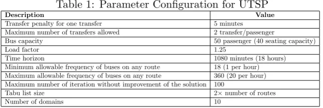
The efficiency of the proposed MTS algorithm is tested on a transit network from Mandl’s Swiss Network. It represents a small transit network with 15 nodes, 21 undirected edges and 15570 total passengers demand (see Fig-ure 3). The MTS algorithm is coded in ANSI-C language and executed on 2.30 GHz Intel(R) Core(TM) i3-2350M CPU with 2GB of RAM under Windows 7 operating system. The pa-rameters for UTSP and MTS used in this study are given in Table 1. A computational exper-iment is conducted for several route sets and compared with the solutions from previous lit-erature.
B. Experimental Results
1. Bus Frequency Optimization
The effectiveness of the proposed MTS algo-rithm for frequency setting problem is evalu-ated using the following performance metrics as suggested by Arbex and da Cunha (2015).
• Total number of buses
Algorithm 1Multiple Tabu Search for Frequency Optimization Xi set of respective frequencies
x current solution x∗ best-known solution k iteration
N(x) neighbourhood ofx F∗ objective value ofx∗ T tabu list
1: BEGIN
2: Variables and functions declaration 3: Passenger assignment procedure
4: Divide the range of frequency intomdomains 5: Fori= 1tom
6: select an initialx∈Xiand setx∗=x, F∗=f(x∗), T=∅, k= 0. 7: whilethere is no improvement inx∗until certain iteration.
8: setk=k+ 1 and generateN(x) by increasing and decreasing the frequency based on adaptive 9: search mechanism.
10: evaluate every solutions inN(x) 11: Ifthere is no feasible solution
12: dointensificationand if intermediate term memory is empty,restartthe process.
13: else
14: choose randomly the bestxfrom an admissible subset (non-dominated solution) ofN(x) which 15: contains non-tabu moves or moves allowed by aspiration criteria. Update the subset.
16: Ifthe subset is empty,
17: dointensificationandifintermediate term memory is empty, select the least worst 18: solution.Ifthere is none, dodiversification.
19: ifF(x)< F∗, then setx∗=xandF∗=F(x). UpdateT and intermediate term memory. 20: end while
21: Record the best solution from each domain 22: End for
23: ReturnBEST
24: END
Algorithm 2Multiple Tabu Search for Bus and Driver Optimization
Xi set of respectively vehicle blocks x current solution (a set of blocks)
x∗ best-known solution (a set of blocks)
k iteration
N(x) neighbourhood ofx F∗ objective value ofx∗ T tabu list
1: BEGIN
2: Variables and functions declaration
3: Divide the set of departure times into m domains. 4: Fori= 1tom
5: select an initialx∈Xiand setx∗=x, F∗=f(x∗), T=∅, k= 0. 6: whilethere is no improvement inx∗until certain iteration.
7: setk=k+ 1 and generateN(x) by adding, dropping and swapping the blocks based on systematic 8: neighborhood search mechanism.
9: evaluate every solutions inN(x) 10: Ifthere is no feasible solution 11: do constraint handling procedure.
12: else
13: choose randomly the bestxfrom an admissible subset (non-dominated solution) ofN(x) which 14: contains non-tabu moves or moves allowed by aspiration criteria. Update the subset.
15: Ifthe subset is empty,
16: dointensificationandifintermediate term memory is empty, select the least worst 17: solution.Ifthere is none, dodiversification.
18: ifF(x)< F∗, then setx∗=xandF∗=F(x). UpdateTand intermediate term memory. 19: end while
20: Record the best solution from each domain 21: End for
22: Reconstruction mechanism 23: ReturnBEST
Table 1: Parameter Configuration for UTSP
Description Value
Transfer penalty for one transfer 5 minutes
Maximum number of transfers allowed 2 transfer/passenger
Bus capacity 50 passenger (40 seating capacity)
Load factor 1.25
Time horizon 1080 minutes (18 hours)
Minimum allowable frequency of buses on any route 18 (1 per hour) Maximum allowable frequency of buses on any route 360 (20 per hour) Maximum number of iteration without improvement of the solution 100
Tabu list size 2×number of routes
Number of domains 10
Figure 3: Mandl’s Swiss Network
• Average route headways
• Maximum route headways
The proposed MTS algorithm is compared
to different algorithms: heuristic by Mandl
(1980), Baaj and Mahmassani (1991), Shih and Mahmassani (1994); genetic algorithm with ant-system (GA-AS) by Bagloee and Ceder (2011); bee colony optimization (BCO)
by Nikoli´c and Teodorovi´c (2014); genetic
al-gorithm (GA) by Arbex and da Cunha (2015); memetic algorithm (MA) by Zhao et al. (2015); and differential evolution (DE) by Buba and Lee (2018). These researchers also contributed
their route sets for this study together with other authors such as Chakroborty (2003), Mumford (2013), Chew et al. (2013). Every researcher has their own optimal sequence of
the nodes in the route set. Therefore, the
solution of the frequency setting problem is based on the route set given. The solution with lower number of buses, lesser total waiting time, lesser average and maximum headways without overcrowding is considered as the best.
The ranking of the performance metrics is categorized such that number of buses is the most important followed by total waiting times, average route headway and maximum
route headway consecutively. The solution
with lower number of buses is given the highest priority to be chosen as the best. Note that, the average values for number of buses are round up to the nearest whole number.
The proposed algorithm is tested with the respective passenger assignment methods and transfer penalties used by the previous authors
for all the route sets. For each route, the
proposed algorithm is conducted for 10 runs to check the robustness of the algorithm based on the parameter configuration in Table 1. Based on the Tables 2 - 7, the first column indicates the source of the route sets to the benchmark data. The second column indicates the algorithms used to obtain the optimal
results. The next five columns specified the
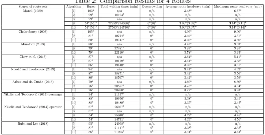
In the case of 4 routes (see Table 2), the proposed MTS algorithms improved the number of buses, total waiting times, average route headways and maximum route headways as compared to the values produced by other authors for all the route sets except Mandl (1980). For the route set from Mandl (1980), although the number of buses is significantly lesser but the total waiting time is higher. The results from the two passenger assignment models are presented for comparison since both of the models are utilized in the past literature. We can also observe that there is no significant difference in the solution from the two models such that they are comparable to each other. Note that although Chakroborty (2003) has published the route sets for 4, 6, 7 and 8 routes but only route 4 is included for comparison because there is no previously
published result available considering the
aforementioned performance criteria for 6, 7 and 8 routes.
For 5 routes, the proposed MTS algorithm is compared with the result only from Arbex and da Cunha (2015) as it is the only study that produced 5 routes for Mandl’s network. From Table 3, MTS algorithm produces better results in term of total number of buses, maximum route headway and average route
headway. In the case of 6 routes, the MTS
algorithms outperformed all the previously published results but the average route head-way for Mumford (2013) is higher since the
number of buses is lower. For the routes in
Baaj and Mahmassani (1991), two passenger assignment method using multinomial logit model and frequency share rule are applied to compare with the respective solutions from literature. The proposed MTS algorithm pro-duced superior results when compared to the existing solutions correspondingly. Besides, for the route sets in Chew et al. (2013) and Arbex and da Cunha (2015), the total waiting times for the best values are higher than the average values since the waiting time can be increased by reducing the number of buses.
In the case of 7 routes, Table 4 shows that the proposed MTS algorithm improves the value of Arbex and da Cunha (2015) for their
own route sets and the routes from Nikoli´c
and Teodorovi´c (2013). The proposed MTS
algorithm outperformed the solutions from Arbex and da Cunha (2015) for the route set of Chew et al. (2013) and the solutions of Buba
and Lee (2018). Besides, our solutions are
comparable to Nikoli´c and Teodorovi´c (2014)
for both operator and passenger and to Arbex and da Cunha (2015) for the Mumford (2013) routes but not in the Pareto sense because the number of buses for the average solution
is higher. Similarly, the results from MTS
algorithm is equivalent to the values from Baaj and Mahmassani (1991). Most of studies have higher total waiting times for average values as compared to the best values due to lower number of buses.
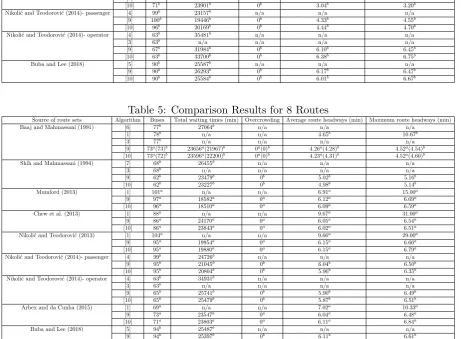
In the case of 8 routes (see Table 5), the proposed MTS algorithm improved the previ-ous solutions for the routes from all the studies
except Arbex and da Cunha (2015). The
number of buses produced by the proposed MTS algorithms are higher but the average and maximum route headway are lower for the routes in Arbex and da Cunha (2015).Alter-natively, the best value of total waiting time for the route set are higher as compared to
the average value. In addition, the average
solutions of MTS algorithm are equivalent to
Nikoli´c and Teodorovi´c (2014) and Zhao et al.
(2015) as the total number of buses is higher even though the total waiting times are lesser.
Furthermore, our proposed MTS algorithm generate best results as compared to Arbex and da Cunha (2015) for 9 and 11 routes (see
Table 6). However, for 11 routes, the best
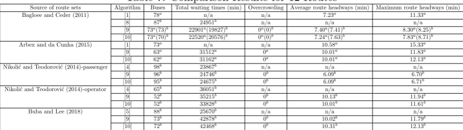
the total buses are increased. Based on Table 7, for 12 routes, our results are preferable as compared to Bagloee and Ceder (2011),
Nikoli´c and Teodorovi´c (2014)-operator and
Arbex and da Cunha (2015) for their respec-tive route sets. Moreover, the results in this study are relatively comparable with Arbex and da Cunha (2015) for the routes from
Bagloee and Ceder (2011) and with Nikoli´c
and Teodorovi´c (2014)-passenger and Buba
and Lee (2018) for their own route sets.
In order to further validate and verify our proposed algorithms, the algorithm is tested using an extended model considering different demands and travel times throughout the time horizon as in peak and off-peak hours. Each of the time intervals between 5.00 am to 11.00 pm are indicated as a timeslot (see Table 8). The parameters are set as in Table 1 and the multinomial logit model is applied for passen-ger assignment procedure. The route sets from Buba and Lee (2018) are experimented and the results for 4 routes of the extended model which includes the average solutions of every domain are presented in Table 9.
Generally, the total buses are dependent on round trip time of a bus. Thus, the number of buses required is quite high as compared to the previous model because the layover time and dwell time are added to the travel time of a bus which increase the round trip time for a trip. Since the frequencies for peak and off-peak hours are not the same, the total waiting times also increases. The existence of overcrowding in the first two domain is caused by insufficient number of bus trip that unable to carry all the passengers at specific timeslot in some of the routes.
The solution from domain 3 which needs lesser number of buses is chosen to study the bus and crew scheduling problem and to build the schedules. This is because there is no over-crowding in the results starting from domain 3 and thus the solutions from domain 3 to 10 are
more preferable.
2. Bus and Driver Scheduling
For bus and driver scheduling, we have studied two different scenarios regarding the departure times at the origin and destination of a route. The first scenario allocate same departure times at both terminals which favors the
travelling passengers. This is to ensure the
headways are equal during the time period
for both terminals. Conversely, the second
scenario assigns the departure times only for the starting terminal.
Each scenario is performed for 10 runs and the average and best solution among them are
recorded. The input data such as frequency
and one-away travel time of the routes are obtained from frequency setting problem. Based on the Tables 10 and 11, the number of buses and drivers required for consecutive trips from one terminal to another are listed according to the number of routes.
The total buses and drivers are increase as the number of routes increase since each route need to be assigned different buses and
drivers. Furthermore, the average and best
solution from both tables are almost equal to each other which shows the robustness of the algorithm.
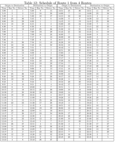
By comparing both scenarios, the total buses and drivers are higher for scenario 1 than scenario 2 because the departure times to be covered are increased as it considers both starting and ending terminals. The bus and driver schedule of scenario 1 for the 4 routes from Buba and Lee (2018) are displayed in
Table 12-15. It shows the bus numbers and
drivers that cover the respective departure times at the first stop (origin) and last stop (destination) of a route.
Based on Table 12, total number of buses and drivers needed for the first route are
Table 2: Comparison Results for 4 Routes
Source of route sets Algorithm Buses Total waiting times (min) Overcrowding Average route headways (min) Maximum route headways (min)
Mandl (1980) [1] 103a n/a n/a 3.48a 6.67a
[2] 99b 18194b n/a n/a n/a
[3] 99b n/a n/a n/a n/a
[9] 54a(55)b 27959a(24666)b 0a(0)b 3.08a(3.05)b 3.14a(3.11)b
[10] 54a(54)b 27563a(24746)b 0a(0)b 3.00a(3.07)b 3.14a(3.14)b
Chakroborty (2003) [1] 105a n/a n/a 4.06a 9.00a
[9] 81a 19724a 0a 3.39a 3.51a
[10] 80a 19247a 0a 3.30a 3.36a
Mumford (2013) [1] 86a n/a n/a 4.43a 9.33a
[9] 79a 22281a 0a 3.82a 3.95a
[10] 79a 22110a 0a 3.78a 3.93a
Chew et al. (2013) [1] 87a n/a n/a 3.64a 5.11a
[9] 87a 19119a 0a 3.44a 3.58a
[10] 86a 19440a 0a 3.50a 3.61a
Nikoli´c and Teodorovi´c (2013) [1] 94a n/a n/a 3.41a 4.32a
[9] 87a 18871a 0a 3.42a 3.56a
[10] 86a 18767a 0a 3.42a 3.59a
Arbex and da Cunha (2015) [1] 79a n/a n/a 4.60a 8.60a
[9] 76a 20857a 0a 3.78a 3.94a
[10] 76a 20780a 0a 3.77a 3.93a
Nikoli´c and Teodorovi´c (2014)-passenger [4] 94b 21147b n/a n/a n/a
[9] 88b 19656b 0b 3.38b 3.49b
[10] 88b 19489b 0b 3.35b 3.47b
Nikoli´c and Teodorovi´c (2014)-operator [1] 67b 26057b n/a n/a n/a
[3] 67b n/a n/a n/a n/a
[9] 54b 25040b 0b 4.29b 4.48b
[10] 54b 24711b 0b 4.24b 4.50b
Buba and Lee (2018) [5] 95b 24098b n/a n/a n/a
[9] 87b 21117b 0b 3.38b 3.53b
[10] 86b 21095b 0b 3.41b 3.61b
Note: n/a=not available; a=multinomial logit model; b=frequency share rule
[l]:Arbex and da Cunha (2015); [2]:Mandl (1980); [3]:Zhao et al. (2015); [4]:Nikoli´c and Teodorovi´c (2014); [5]:Buba and Lee (2018); [6]:Baaj and Mahmassani (1991); [7]:Shih and Mahmassani (1994); [8]:Bagloee and Ceder (2011); [9]:proposed MTS(average); [10]:proposed MTS(best)
Table 3: Comparison Results for 5 and 6 Routes
Source of route sets Algorithm Buses Total waiting times (min) Overcrowding Average route headways (min) Maximum route headways (min)
5 routes
Arbex and da Cunha (2015) [1] 75a n/a n/a 5.39a 9.56a
[9] 66a 25660a 0a 5.17a 5.45a
[10] 64a 26262a 0a 5.26a 5.48a
6 routes
Baaj and Mahmassani (1991) [6] 89b 20920b n/a n/a n/a
[1] 87a n/a n/a 4.11a 11.33a
[3] 89b n/a n/a n/a n/a
[9] 76a(76)b 20862a(19655)b 0a(0)b 3.36a(3.36)b 3.46a(3.45)b
[10] 76a(76)b 20782a(19558)b 0a(0)b 3.35a(3.35)b 3.44a(3.44)b
Shih and Mahmassani (1994) [7] 84b 20058b n/a n/a n/a
[3] 84b n/a n/a n/a n/a
[9] 82b 19957b 0b 3.06b 3.13b
[10] 82b 19869b 0b 3.04b 3.09b
Mumford (2013) [1] 98a n/a n/a 5.06a 8.00a
[9] 88a 18469a 0a 5.08a 5.31a
[10] 88a 18433a 0a 5.08a 5.24a
Chew et al. (2013) [1] 110a n/a n/a 4.86a 8.00a
[9] 104a 16626a 0a 4.37a 4.59a
[10] 101a 17457a 0a 4.56a 4.74a
Nikoli´c and Teodorovi´c (2013) [1] 102a n/a n/a 5.25a 10.29a
[9] 100a 18178a 0a 4.58a 4.83a
[10] 100a 18147a 0a 4.52a 4.70a
Nikoli´c and Teodorovi´c (2014)-passenger [4] 99b 21766b n/a n/a n/a
[9] 98b 19800b 0b 3.78b 3.91b
[10] 98b 19697b 0b 3.76b 3.87b
Nikoli´c and Teodorovi´c (2014)- operator [4] 66b 31500b n/a n/a n/a
[3] 66b n/a n/a n/a n/a
[9] 61b 26162b 0b 4.30b 4.52b
[10] 61b 25946b 0b 4.27b 4.43b
Arbex and da Cunha (2015) [1] 77a n/a n/a 6.42a 9.56a
[9] 66a 22994a 0a 6.06a 6.55a
[10] 63a 26728a 0a 6.31a 6.71a
Buba and Lee (2018) [5] 92b 24705b n/a n/a n/a
[9] 85b 23117b 0b 5.07b 5.34b
[10] 85b 23091b 0b 5.04b 5.57b
(number of departure time) at each terminal is 99 with the average headway of 11.79 minutes. Each departure time is assigned to a specific bus and driver according to the travel time
and working period. The frequency of the
Table 4: Comparison Results for 7 Routes
Source of route sets Algorithm Buses Total waiting times (min) Overcrowding Average route headways (min) Maximum route headways (min)
Mumford (2013) [1] 102a n/a n/a 5.32a 6.80a
[9] 105a 15996a 0a 5.11a 5.42a
[10] 101a 16446a 0a 5.25a 5.51a
Chew et al. (2013) [1] 110a n/a n/a 4.86a 8.00a
[9] 112a 16350a 0a 4.32a 4.54a
[10] 108a 17077a 0a 4.50a 4.74a
Nikoli´c and Teodorovi´c (2013) [1] 98a n/a n/a 7.00a 17.5a
[9] 82a 21501a 0a 6.12a 6.60a
[10] 82a 21458a 0a 6.13a 6.63a
Arbex and da Cunha (2015) [1] 77a n/a n/a 7.58a 12.8a
[9] 76a 22323a 0a 6.18a 6.74a
[10] 76a 21955a 0a 6.12a 6.84a
Baaj and Mahmassani (1991) [6] 82b 22804b n/a n/a n/a
[3] 82b n/a n/a n/a n/a
[9] 72b 23893b 0b 3.03b 3.11b
[10] 71b 23901b 0b 3.04b 3.20b
Nikoli´c and Teodorovi´c (2014)- passenger [4] 99b 23157b n/a n/a n/a
[9] 100b 19446b 0b 4.33b 4.55b
[10] 96b 20169b 0b 4.44b 4.70b
Nikoli´c and Teodorovi´c (2014)- operator [4] 63b 35481b n/a n/a n/a
[3] 63b n/a n/a n/a n/a
[9] 67b 31984b 0b 6.10b 6.45b
[10] 63b 33700b 0b 6.38b 6.75b
Buba and Lee (2018) [5] 90b 25587b n/a n/a n/a
[9] 90b 26293b 0b 6.17b 6.47b
[10] 90b 25584b 0b 6.01b 6.67b
Table 5: Comparison Results for 8 Routes
Source of route sets Algorithm Buses Total waiting times (min) Overcrowding Average route headways (min) Maximum route headways (min)
Baaj and Mahmassani (1991) [6] 77b 27064b n/a n/a n/a
[1] 78b n/a n/a 4.65b 10.67b
[3] 77b n/a n/a n/a n/a
[9] 73a(73)b 23656a(21967)b 0a(0)b 4.26a(4.28)b 4.52a(4.54)b
[10] 73a(72)b 23596a(22200)b 0a(0)b 4.23a(4.31)b 4.52a(4.60)b
Shih and Mahmassani (1994) [7] 68b 26455b n/a n/a n/a
[3] 68b n/a n/a n/a n/a
[9] 62b 23479b 0b 5.02b 5.16b
[10] 62b 23227b 0b 4.98b 5.14b
Mumford (2013) [1] 101a n/a n/a 6.91a 15.00a
[9] 97a 18582a 0a 6.12a 6.69a
[10] 96a 18510a 0a 6.09a 6.59a
Chew et al. (2013) [1] 88a n/a n/a 9.67a 31.00a
[9] 86a 24170a 0a 6.05a 6.54a
[10] 86a 23843a 0a 6.02a 6.51a
Nikoli´c and Teodorovi´c (2013) [1] 104a n/a n/a 9.66a 29.00a
[9] 95a 19954a 0a 6.15a 6.66a
[10] 95a 19880a 0a 6.15a 6.79a
Nikoli´c and Teodorovi´c (2014)- passenger [4] 99b 24726b n/a n/a n/a
[9] 95b 21045b 0b 6.04b 6.50b
[10] 95b 20804b 0b 5.96b 6.35b
Nikoli´c and Teodorovi´c (2014)- operator [4] 63b 34931b n/a n/a n/a
[3] 63b n/a n/a n/a n/a
[9] 65b 25741b 0b 5.90b 6.49b
[10] 65b 25479b 0b 5.87b 6.51b
Arbex and da Cunha (2015) [1] 69a n/a n/a 7.02a 10.33a
[9] 73a 23547a 0a 6.04a 6.48a
[10] 71a 23803a 0a 6.11a 6.84a
Buba and Lee (2018) [5] 94b 25487b n/a n/a n/a
[9] 94b 25397b 0b 6.11b 6.61b
[10] 93b 25083b 0b 6.11b 6.79b
Table 6: Comparison Results for 9,10 and 11 Routes
Source of route sets Algorithm Buses Total waiting times (min) Overcrowding Average route headways (min) Maximum route headways (min)
9 routes
Arbex and da Cunha (2015) [1] 66a n/a n/a 9.14a 20.00a
[9] 58a 35226a 0a 7.51a 8.26a
[10] 58a 34381a 0a 7.34a 8.06a
10 routes
Arbex and da Cunha (2015) [1] 72a n/a n/a 9.44a 20.00a
[9] 81a 23990a 0a 7.43a 8.16a
[10] 81a 23903a 0a 7.36a 7.88a
11 routes
Arbex and da Cunha (2015) [1] 68a n/a n/a 8.76a 14.4a
[9] 70a 26032a 0a 7.38a 8.01a
Table 7: Comparison Results for 12 Routes
Source of route sets Algorithm Buses Total waiting times (min) Overcrowding Average route headways (min) Maximum route headways (min)
Bagloee and Ceder (2011) [1] 78a n/a n/a 7.23a 11.33a
[8] 87b 24951b n/a n/a n/a
[9] 73a(73)b 22901a(19827)b 0a(0)b 7.40a(7.41)b 8.30a(8.25)b
[10] 73a(70)b 22520a(20576)b 0a(0)b 7.24a(7.63)b 7.83a(8.71)b
Arbex and da Cunha (2015) [1] 73a n/a n/a 10.58a 15.33a
[9] 63a 31512a 0a 10.01a 11.83a
[10] 62a 31162a 0a 10.01a 12.13a
Nikoli´c and Teodorovi´c (2014)-passenger [4] 98b 23867b n/a n/a n/a
[9] 96b 24746b 0b 6.09b 6.70b
[10] 95b 24675b 0b 6.09b 6.71b
Nikoli´c and Teodorovi´c (2014)-operator [4] 65b 36051b n/a n/a n/a
[9] 52b 35215b 0b 10.13b 11.94b
[10] 52b 33828b 0b 10.01b 11.61b
Buba and Lee (2018) [5] 88b 25670b n/a n/a n/a
[9] 73b 42878b 0b 10.02b 11.79b
[10] 72b 42468b 0b 10.31b 12.13b
Table 8: Category of each Timeslot
Timeslot Time interval Category
1 0500-0600 Off-peak
2 0600-0700 Off-peak
3 0700-0800 Peak
4 0800-0900 Peak
5 0900-1000 Peak
6 1000-1100 Off-peak
7 1100-1200 Off-peak
8 1200-1300 Peak
9 1300-1400 Peak
10 1400-1500 Off-peak
11 1500-1600 Off-peak
12 1600-1700 Peak
13 1700-1800 Peak
14 1800-1900 Peak
15 1900-2000 Peak
16 2000-2100 Off-peak
17 2100-2200 Off-peak
18 2200-2300 Off-peak
Table 9: Results Obtained for Extended Model for 4 Routes
Domain Number of buses Total waiting times (min) Overcrowding
1 17 260559 6034
2 31 139851 731
3 44 99934 0
4 58 76488 0
5 70 62809 0
6 83 52725 0
7 97 45625 0
8 109 40419 0
9 122 36097 0
10 136 29406 0
minutes of interval.
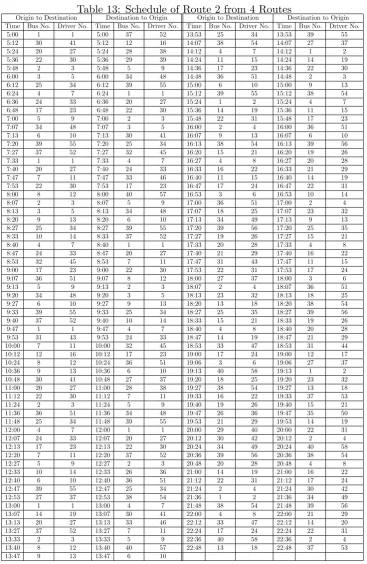
Table 13 shows that route 2 require 40 buses and 58 drivers to cover all the departure
times between 5.00 am and 11.00 pm. The
total departure times at each terminal is 126 with the average headway of 9.34 minutes. The frequency and headway of the route at
Table 10: Results for scenario 1 (Buba and Lee, 2018)
Routes Algorithm Total buses Total crews
4 Average 110 154
Best 106 153
6 Average 151 207
Best 148 203
7 Average 195 254
Best 191 254
8 Average 206 250
Best 202 268
12 Average 258 355
Best 256 349
Table 11: Results for scenario 2 (Buba and Lee, 2018)
Routes Algorithm Total buses Total crews
4 Average 103 136
Best 98 134
6 Average 137 185
Best 134 179
7 Average 175 227
Best 165 226
8 Average 185 242
Best 179 239
12 Average 240 312
Best 234 310
peak hours is 9 and 6.67 minutes respectively. Meanwhile, the frequency and headway of the route at off-peak hours are 5 and 12 minutes correspondingly.
as-Table 12: Schedule of Route 1 from 4 Routes
Origin to Destination Destination to Origin Origin to Destination Destination to Origin Time Bus No. Driver No. Time Bus No. Driver No. Time Bus No. Driver No. Time Bus No. Driver No.
5:00 1 1 5:00 9 15 13:51 25 36 13:51 11 19
5:15 2 2 5:15 18 28 14:00 7 11 14:00 23 34
5:30 3 4 5:30 10 17 14:15 22 33 14:15 2 2
5:45 25 36 5:45 4 6 14:30 6 9 14:30 12 21
6:00 19 29 6:00 1 1 14:45 11 19 14:45 25 36
6:15 18 28 6:15 2 2 15:00 23 34 15:00 7 11
6:30 8 13 6:30 3 4 15:15 2 3 15:15 22 33
6:45 11 19 6:45 25 36 15:30 12 21 15:30 6 9
7:00 1 1 7:00 19 29 15:45 21 32 15:45 11 19
7:09 2 2 7:09 18 28 16:00 7 11 16:00 8 14
7:17 3 4 7:17 8 13 16:09 22 33 16:09 2 3
7:26 5 7 7:26 6 9 16:17 6 9 16:17 12 21
7:34 25 36 7:34 11 19 16:26 10 18 16:26 21 32
7:43 22 33 7:43 21 32 16:34 13 22 16:34 14 23
7:51 19 29 7:51 1 1 16:43 8 14 16:43 7 11
8:00 18 28 8:00 2 2 16:51 20 30 16:51 15 24
8:09 8 13 8:09 3 4 17:00 2 3 17:00 16 25
8:17 6 9 8:17 5 7 17:09 5 8 17:09 6 10
8:26 11 19 8:26 25 36 17:17 3 5 17:17 9 16
8:34 17 26 8:34 22 33 17:26 14 23 17:26 13 22
8:43 1 1 8:43 19 29 17:34 7 11 17:34 8 14
8:51 2 2 8:51 18 28 17:43 15 24 17:43 20 30
9:00 3 4 9:00 8 13 17:51 16 25 17:51 2 3
9:09 5 7 9:09 6 9 18:00 6 10 18:00 5 8
9:17 25 36 9:17 11 19 18:09 12 21 18:09 10 18
9:26 22 33 9:26 17 26 18:17 13 22 18:17 14 23
9:34 19 29 9:34 23 34 18:26 8 14 18:26 7 11
9:43 4 6 9:43 1 1 18:34 20 30 18:34 15 24
9:51 8 13 9:51 3 4 18:43 17 27 18:43 16 25
10:00 6 9 10:00 5 7 18:51 5 8 18:51 6 10
10:15 11 19 10:15 20 30 19:00 10 18 19:00 12 21
10:30 17 26 10:30 22 33 19:09 14 23 19:09 13 22
10:45 18 28 10:45 2 2 19:17 24 35 19:17 3 5
11:00 5 7 11:00 6 9 19:26 15 24 19:26 20 31
11:15 9 15 11:15 25 36 19:34 16 25 19:34 17 27
11:30 22 33 11:30 17 26 19:43 2 3 19:43 5 8
11:45 2 2 11:45 8 13 19:51 12 21 19:51 10 18
12:00 1 1 12:00 19 29 20:00 13 22 20:00 14 23
12:09 25 36 12:09 11 19 20:15 7 11 20:15 15 24
12:17 17 26 12:17 23 34 20:30 17 27 20:30 16 25
12:26 8 13 12:26 2 2 20:45 26 37 20:45 12 21
12:34 21 32 12:34 12 21 21:00 10 18 21:00 24 35
12:43 6 9 12:43 5 7 21:15 11 20 21:15 7 11
12:51 26 37 12:51 4 6 21:30 2 3 21:30 17 27
13:00 11 19 13:00 25 36 21:45 3 5 21:45 26 37
13:09 23 34 13:09 7 11 22:00 14 23 22:00 13 22
13:17 2 2 13:17 22 33 22:15 7 12 22:15 11 20
13:26 12 21 13:26 21 32 22:30 16 25 22:30 2 3
13:34 5 7 13:34 6 9 22:45 20 31 22:45 3 5
13:43 4 6 13:43 26 37
signed at every departure time in route 3. The schedule consists of 21 buses and 31 drivers. The time intervals between every departure time are set at 6.67 minutes for peak hours and 12 minutes for off-peak hours. Thus, the number of bus departure for peak hours and off-peak hours are 9 and 5 respectively. The average headway of the route is 9.34 minutes.
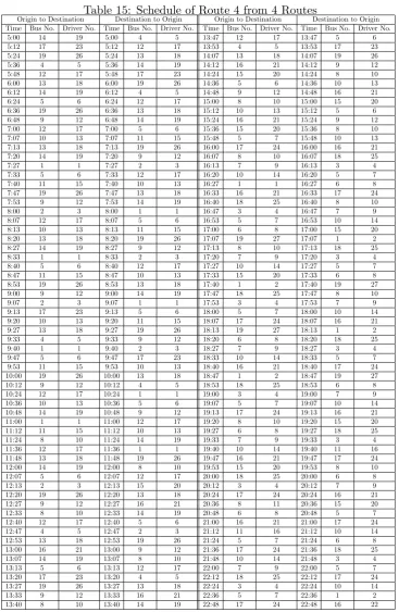
Similarly, Table 15 presents the sequence of 126 departure times at each terminal of
route 4. A total of 19 buses and 27 drivers
are allocated to the departure times. The
frequency and headway of the route at peak hours are fixed as 9 and 6.67 minutes. During off-peaks hours, the frequency and headway are scheduled at 5 and 12 minutes respectively.