Published online February 20, 2013 (http://www.sciencepublishinggroup.com/j/ajsea) doi: 10.11648/j. ajsea.20130201.13
Generic object recognition using graph embedding into a
vector space
Takahiro Hori, Tetsuya Takiguchi, Yasuo Ariki
Graduate School of System Informatics, Kobe University, Japan
Email address:
[email protected] (T. Hori), [email protected] (T. Takiguchi), [email protected] (Y. Ariki)
To cite this article:
Takahiro Hori, Tetsuya Takiguchi, Yasuo Ariki. Generic Object Recognition Using Graph Embedding into a Vector Space, American Journal of Software Engineering and Applications. Vol. 2, No. 1, 2013, pp. 13-18. doi: 10.11648/j.ajsea.20130201.13
Abstract: This paper describes a method for generic object recognition using graph structural expression. In recent years,
generic object recognition by computer is finding extensive use in a variety of fields, including robotic vision and image retrieval. Conventional methods use a bag-of-features (BoF) approach, which expresses the image as an appearance frequency histogram of visual words by quantizing SIFT (Scale-Invariant Feature Transform) features. However, there is a problem associated with this approach, namely that the location information and the relationship between keypoints (both of which are important as structural information) are lost. To deal with this problem, in the proposed method, the graph is constructed by connecting SIFT keypoints with lines. As a result, the keypoints maintain their relationship, and then structural representation with location information is achieved. Since graph representation is not suitable for statistical work, the graph is embedded into a vector space according to the graph edit distance. The experiment results on two image datasets of multi-class showed that the proposed method improved the recognition rate.Keywords: Generic Object Recognition, Graph Edit Distance, SIFT
1. Introduction
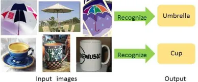
Generic object recognition means that the computer recognizes objects real world images by their general name (see Fig. 1). It is one of most challenging tasks in the field of computer vision. Regarding the achieving of near-human vision by a computer, it is expected that any such technology will be applied to robotic vision. Moreover, due to the spread of digital cameras and the development of high-capacity hard disk drives in recent years, it is getting difficult to classify and to retrieve large-volume videos and images manually. Therefore, computers are being looked at to assist in automatically classifying and retrieving videos and images. In particular, generic object recognition is becoming more and more important.
Figure 1. Generic object recognition.
There have been two typical approaches in the past concerning general object recognition. One is a method based on image segmentation. This is a technique for automatic annotation to the segmented image area, word-image-translation model by Barnard [1, 2, 3]. However, when the image has occlusion and the image segmentation fails, it becomes difficult for this technique to work correctly.
On the other hand, to solve this problem, a method based on the local pattern is proposed. This is a technique for collating the image by combining local features of the image. The technique for characterizing the entire image is often used for the appearance frequency histogram of the localizing features (known as Bag of Features, as shown in Fig. 2 [4]). However, there is a problem with this approach because the location information and the relationships between keypoints are lost.
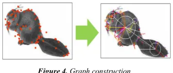
To deal with this problem, we propose a method in this paper to connect keypoints with lines, as shown in Fig. 4, and to express the sets of the local features as a graph. Moreover, we propose a technique with high recognition performance that integrates the object structure and the local features by embedding the graph into a vector space using the graph edit distance (GED). Thus, the objects are expressed by a simple vector of the statistical work, and trained and classified by Support Vector Machine (SVM). The results of our object recognition experiments show the effectiveness of our method.
Figure 4. Graph construction.
This paper is organized as follows. In Sections 2, 3, 4, and 5, the proposed method is described. In Section 6, the performance of the proposed method is evaluated for a 10-class image dataset. Section 7 provides a summary and discusses future work.
2. Overview of the Proposed Method
Fig. 3 shows the system overview. First, the SIFT keypoints and features [5] of all images are extracted. The extracted keypoints are connected and a graph of each image is constructed. The graphs constructed from the training images are called training graphs and those of the test images test graphs. Next, n prototype graphs are selected from the training graphs, and GED is calculated n times between the prototype graphs and each graph (training graphs and test graphs). Thus, the graphs are embedded into an n-dimensional vector space. The classifier is trained by the n-dimensional vectors of the training images. Finally, the test data is classified by the trained classifier and the recognition result is output. In the following sections, each process in the proposed method is described in detail.
Figure 3. System overview.
3. Graph Structural Expression
In this paper, we use the notation and structural representation of the graph proposed in [6]. In the formalization, the graph is noted as G = (V, E, X) where E represents the set of edges, V is the set of vertices and X the set of their associated unary measurements (in our case, a SIFT descriptor). The node is a keypoint detected by SIFT, and the associated unary measurements represent the 128-dimension SIFT descriptor of the corresponding keypoints. Hence, prototype graphs Gp and other graphs (called scene graph Gs) are distinguished. Similarly, we denote the set of nodes of the prototype graph by
, , … , , … (1) whereas the nodes of the scene graph are written with
, , … , , … 2 Note that the subscript variables associated to the nodes also differ: we have used a Latin subscript for the scene nodes and a Greek subscript for prototype nodes. The associated unary measurements x and x are treated the same way. Also, an edge between two nodes and is denoted as ( for an edge of the scene graph). Finally, the assignment of a scene node to a prototype node during the matching process is represented with the notation .
3.1. Proximity Graph
It is a complete graph if all the keypoints extracted from the image are connected mutually by the edges. However, it is not usually suitable for the calculation. Additionally, because the relationships between keypoints over a long distance are weak, it is preferable to connect them only within their "neighborhood." Thus, we simply define the proximity graph as a graph in which distant keypoints are not connected. Formally, we restrain the set of edges to:
E , "#$%#&"
'($(& ) * + (3)
where p -., -/ denotes a keypoint position, σ its scale, and χ is a constant. By this definition, the larger scale keypoints connect to the more distant keypoints. The edge is not drawn in case where the value is longer than constant χ. Because an extra edge is not drawn by this constraint, the constructed proximity graph reduces the computation load considerably, and improves the detection performance at the same time. Both the prototype graphs and the scene graphs are constructed as proximity graphs.
3.2. Pseudo-Hierarchical Graph
down the hierarchy gradually. We decompose the graph into a set of subgraphs 23 345 based on the scale of the keypoints. For each level l, only the features whose scale is superior to a threshold 63 are retained.
63 78 9:(;<=(;$>%(;$>?
@AB
@AC (4)
where 78D. and 78 9 are the maximum and minimum scale of the keypoints in each graph. Fig. 5 shows an example of subgraph 23 34E divided into three
hierarchical levels. Note that only the prototype graphs are decomposed to the pseudo-hierarchical graphs.
Figure 5. Pseudo-Hierarchical Graph.
4. Graph Edit Distance
The process of evaluating the structural similarity of two graphs is generally referred to as graph matching. This issue has been addressed by a large number of studies [7]. We use the graph edit distance [8, 9], one of the most widely used methods, to compute the difference between two graphs [10, 11, 12]. A pseudo-hierarchical graph is employed in order to improve the computational complexity of graph edit distance.
The basic idea of the graph edit distance is to define the difference of two graphs as the minimum amount of edit operations required to transform one graph into the other. Namely, it is computed using the number of edit operations composed of insertion, deletion, and substitution of nodes and edges. Two graphs 2 and 2 have the edit path
F 2 , 2 = G , … , GH (each G indicates the edit operation) to convert 2 into 2 using specific editing. Fig. 6 shows the example of an edit path between two graphs 2 and 2 . Each edit cost c is defined as the amount of the distortion in the transformation. The graph edit distance between graphs 2 and 2 is computed as
Figure 6. An edit path between two graphs.
I 2 , 2 minMNC,…,MNO P QC,QR ∑ TH4 G (5)
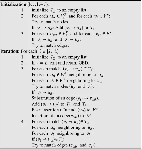
where T G denotes the penalty cost of the edit operation G. The final complete matching procedure is summarized in Fig. 7.
Initialization (level l=1):
1. Initialize U to an empty list.
2. For each and for each :
Try to match nodes.
If : Add ( ) to U.
3. For each V and for each V:
If and :
Try to match edges.
Iteration: For each W X2. . Z[
1. Initialize U to an empty list. 2. If W Z: exit and return GED.
3. For each match U:
For each 3 neighboring to : For each neighboring to ; Try to match nodes ( and ).
If :
Substitution of an edge ( ). Add ( ) to U and U. Else: Insertion of a node( ) to . Insertion of an edge( ) to V.
4. For each match ( ) U:
For each neighboring to : For each neighboring to :
If ( ) U:
Try to match edges ( and ).
Figure 7. Graph edit distance algorithm.
5. Graph Embedding in a Vector Space
The embedding method used in this paper follows the procedure proposed by [13]. This technique is used for the computation of the median graph etc., and the effectiveness is shown in [14, 15]. The approach is described as follows, and the outline is shown in Fig. 8. We prepare a set of the training graphs U 2 , 2 , … , 29 , and compute the graph edit distance I 2 , 2 (, 1, … , ]; 2 , 2 U). First, the set of the m prototype graphs
_ 2 , 2 , … , 28 is selected from T (` a ]). Next, the
graph edit distance between scene graph 2 and prototype graphs 2 _ is calculated. As a result, the m graph edit distances I , … , I8 (IH I 2 , 2H ) to the scene graph are obtained and assumed to form the m dimensional vector D. Thus, all scene graphs 2 can be embedded into the m dimensional vector space by using prototype graph set P. It can be described as follows:
Figure 8. Graph embedding in a vector space.
b: 2 Re (6)
b If2 , 2 g, If2 , 2 g, … , I 2 , 28 (7)
a set of the prototype graphs P is selected from a set of the training graphs T.
6. Experimental Evaluation
6.1. Experimental Conditions
We used the Caltech-101 Database and the PASCAL Visual Object Challenge (VOC) 2007 dataset for the experiment.
The Caltech-101 is composed of 101 classes, used for generic object recognition. We selected 10 object classes from among these 101 classes, and carried out comparative experiments between the proposed method and conventional methods (BoF). The examples of images used in the experiment are shown in Fig. 9. The training images were 30 images randomly selected from each class and the remaining images were used as the test images. In total, 300 training images and 541 test images were used for the 10 classes.
Figure 9. Caltech-101 dataset.
The PASCAL VOC dataset consists of 9,963 images containing at least one instance of each 20 object categories. It is a benchmark for the general object recognition. These images range between indoor and outdoor scenes, close-ups and landscapes, and strange viewpoints. The dataset is more difficult than Caltech-101 because all the images where the size, viewing angle, illumination, etc. appearances of objects and their poses vary significantly, with frequent occlusions. In the experiment, we used the images cut out from the original one by its bounding boxes. We randomly selected 10 object classes, and carried out comparative experiments using 4,986 training images and 4,963 test images. The examples of images of PASCAL are shown in Fig. 10.
Figure 10. PASCAL Visual Object Challenge (VOC) 2007 dataset.
The threshold χ, hierarchical level L of
pseudo-hierarchical graphs, and edit cost c of the graph edit distance were used as the best value in the experiment. As a set of the prototype graphs, a set of the training graphs employed for the Caltech tasks. Because the number of training images was 300, all the images were embedded into the 300 dimension vector spaces. For the PASCAL tasks, the 50 prototype graphs are randomly selected from the training images of each class. On the other hand, the codebook size of the BoF method was 1,000, the best value in the experiment. We used as the classifiers k-Nearest Neighbor algorithm (k=10) and multi-class SVM (linear and radial basis function (RBF)) [16] to classify the vector formed by each method.
6.2. Experimental Results and Discussion
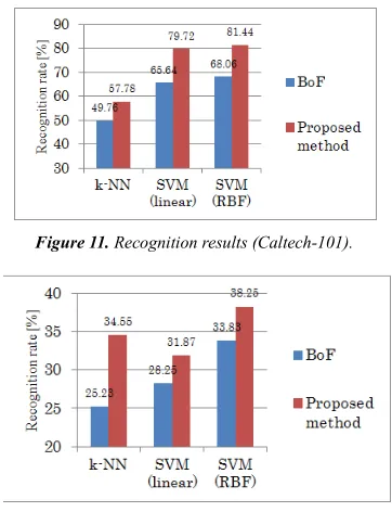
Fig. 11 and Fig. 12 show the recognition results for all classes. As shown these figures, it can be confirmed that the proposed method improved the accuracy. The recognition rate has improved with SVM (RBF) by 13.38%, SVM (linear) by 14.08%, and k-NN by 8.02% in the Caltech tasks, and SVM (RBF) by 4.42%, SVM (linear) by 3.62%, and k-NN by 9.32% in the Pascal tasks, compared to the conventional method BoF.
Figure 11. Recognition results (Caltech-101).
Figure 12. Recognition results (PASCAL).
Figure 14. Recognition results of each class using SVM (RBF).
Figure 15. Recognition results of each class using SVM (linear).
Figure 16. Recognition results of each class using k-NN.
This is because the conventional method uses only SIFT features, so it is strongly influenced by the accuracy of these features. The SIFT features respond strongly to the corners and intensity gradients, so it is not appropriate when they are scarce. In contrast, the proposed method can represents the shape and structure of the object using the graph. Fig. 13 shows the images that was recognized by the proposed method and was not recognized by the conventional method.
Figure 13. Examples of images which were recognized using the proposed method and were not recognized using the conventional method.
In Fig. 16, the recognition rates of accordion, car side, dalmatian, and dollar bill were decreased compared with BoF. However, this decrease is improved in Fig. 14 and Fig. 15. Therefore, the proposed method with SVM can demonstrate the better performance.
Figure 13. Examples of images which were recognized using the proposed method and were not recognized using the conventional method.
7. Conclusion
In this paper, we proposed a new method to recognize generic objects by incorporating graph structural expression by embedding a graph into the vector spaces. By employing the graph structure of the object, the class recognition became robust to the SIFT features variance. As a result, the recognition accuracy was improved considerably compared to the conventional method in the experiments of two datasets. In the future, we will study the selection method of more effective prototype graphs and the method of reducing calculation cost for graph edit distance. Moreover, we are planning to extend this proposed method to three-dimensional graphs and general object recognition using three-dimensional information.
References
[1] K. Barnard and D. A. Forsyth, “Learning the semantics of words and pictures,” Proc. of IEEE International Conf. on Computer Vision, pp. 408–415, 2001.
[2] K. Barnard, P. Duygulu, N. de Freitas, and D. Forsyth, “Matching words and pictures,” Journal of Machine Learning Research, vol. 3, pp. 1107–1135, 2003.
[3] P. Duygulu, K. Barnard, N. de Freitas, and D. Forsyth, “Visual categorization with bags of keypoints,” Proc. of European Conference on Computer Vision, pp. 97–112, 2002.
[4] G. Csurka, C.R. Dance, L. Fan, J. Willamowski, and C. Bray, “Object Recognition as Machine Translation: Learning Lexicons for a Fixed Image Vocabulary,” Proc. of ECCV workshop on Statistical Learning in Computer Vision, pp. 1–22, 2004.
[5] D. G. Low, “Distinctive image features from scale invariant keypoints,” Journal of Computer Vision, vol. 60, pp. 91–110, 2004.
Proc. of Conference on Image and Video Retrieval, pp. 414–421, 2010.
[7] D. Conte, P. Foggia, C. Sansone, and M. Vento, “Thirty years of graph matching in pattern recognition,” International Journal of Pattern Recognition and Artificial Intelligence, vol. 8, pp. 265–298, 2004.
[8] H. Bunke and G. Allerman, “Inexact graph matching for structural pattern recognition,” Pattern Recognition Letters, vol. 1, pp. 245–253, 1983.
[9] A. Sanfeliu and K. Fu, “A distance measure between attributed relational graphs for pattern recognition,” IEEE Transactions on Systems, Man, and Cybernetics, vol. 13, pp. 353–362, 1983.
[10] D. Justice and A. Hero, “A Binary Linear Programming Formulation of the Graph Edit Distance,” IEEE Transactions on Pattern Analysis and Machine Intelligence, vol. 28, pp. 1200–1214, 2006.
[11] M. Neuhaus, K. Riesen, and H. Bunke, “Fast suboptimal algorithms for the computation of graph edit distance,” Joint IAPR International Workshops, SSPR and SPR 2006, Lecture Notes in Computer Science, vol. 4109, pp. 163–172,
2006.
[12] K. Riesen and H. Bunke, “Approximate graph edit distance computation by means of bipartite graph matching,” Image and Vision Computing, vol. 27, pp. 950–959, 2009.
[13] K. Riesen, M. Neuhaus, and H. Bunke, “Graph Embedding in Vector Spaces by Means of Prototype Selection,” Graph-based representations in pattern recognition (GbRPR), F. Escolano et al, Ed., Springer-Verlag Berlin, Heidelberg, pp. 383–393, 2007.
[14] E. Valveny and M. Ferrer, “Application of Graph Embedding to solve Graph Matching Problems,” Proc. of CIFED, pp. 13–18, 2008.
[15] M. Ferrer, E. Valveny, F. Serratosa, K. Riesen, and H.Bunke, “Generalized median graph computation by means of graph embedding in vector spaces,” Pattern Recognition, vol. 43, pp. 1642–1655, 2010.