STORAGE YIELD FUNCTIONS FOR
RAVISANKAR SAGAR RESERVOIR IN
MRP COMPLEX – A Case Study
1ANANDA BABU. K.,
Associate Professor, Civil Engineering Department, Shri Vaishnav Institute of Technology and Science, Indore
Address: 55-56, Flat No.101, O.P.Adhar Aptt. Veena Nagar, Near Bombay Hospital, Indore. 452010
2
Dr. R.K.SHRIVASTAVA,
Professor, Civil Engineering and Applied Mechanics Department, Shri Govindram Sexaria Institute of Technology and Science, Indore
Address: Flat No. 01, Professors Quarters, SGSITS Campus, 23, Park Road, Indore 452001
ABSTRACT
Creation of storages through development of Reservoirs is the major avenue for meeting the water demands for various beneficial uses for a country like India which 90-95% water is available in monsoon months only. The optimal utilization of available resource seems to be the key for tackling the Complex situation of meeting the ever increasing demand of water. Development of strategies for operating a Reservoir in an optimal manner to have the judicious use of available resource is also a complex phenomenon and required the use of System Analysis Techniques. There is no general algorithm for all Reservoirs, and is to be tackled independently for developing the optimal operating strategies. The present study is focused on development of Monthly storage Yield Functions for Ravishankar Sagar Reservoir of Mahanadi Reservoir Complex (MRP) in Raipur District of Chattisgarh State in India using Stochastic Dynamic Programming Model of Loucks et al (1981).
KEYWORDS
Stochastic dynamic programming; Dynamic Programming; Storage Yield Functions; Optimization; Reservoir operation.
INTRODUCTION STUDY AREA:
The Mahanadi is one of the important river systems in the country and is classified amongst the twelve major river basins. Mahanadi Reservoir Project (MRP) complex is situated in the upper reaches of river Mahanadi. At its ultimate stage of development the MRP complex will comprise of six Reservoirs, two major diversion works, and three feeder canals along with three service canals. Inter-basin transfer of water from Pairi-Mahanadi Link Canal (PMLC). The project complex serves the purposes of municipal and Industrial supply and irrigation supplies in a pre-specified priority order. Thus MRP is a multipurpose multi Reservoir system. To mitigate the shortfalls in the supply of water various optimal demands in the system, it is necessary to chalk out the aim of the evaluation of a satisfactory and efficient operating procedure for such a large sized and real-life multipurpose multi Reservoir, mathematical model have been developed and applied in the present study.
Catchment Area at Dam-sites and Diversion works (sq.Km.):
S.No. Name of the Site Gross Intercepted Unintercepted
1 Rudri Weir (Old) 3700 3670 30
2 New Rudri Barrrage 3700 3670 30
3 Ravishankar Sagar Dam 3670 1105 2565
4 Dudhawa Dam 621 Nil 621
5 Murumsilli Dam 484 Nil 484
6 Sondur Dam 512 Nil 512
7 Sikasar Dam 492 Nil 492
8 Pairi Dam 3056 1004 2052
Reservoir Capacities in Mm3:
S.No. Reservoir Storage Capacity at Live Storage
MWL FRL DSL
1 Ravishankar sagar Dam 1223 909 144 765
2 Dudhawa Dam 467 288 4 284
3 Murumsilli Dam 179 15 3 162
4 Sondur Dam 226 180 18 162
5 Sikasar Dam 272 217 18 199
6 Pairi Dam 620 540 120 420
Municipal and Industrial Demands in Mm3:
S.No. Month Municipal Demand Industrial Demand Total M&I Demand
1 June 11.0 3.0 14.0
2 July 0.0 26.0 26.0
3 August 0.0 9.0 9.0
4 Sept. 0.0 10.0 10.0
5 October 0.0 20.0 20.0
6 Nov. 4.0 00.0 4.0
7 Dec. 5.0 00.0 5.0
8 January 6.0 34.0 40.0
9 February 7.0 34.0 41.0
10 March 8.0 34.0 42.0
11 April 9.0 34.0 43.0
12 May 11.0 34.0 44.0
Total 61.0 238.0 299.0
STOCHASTIC DYNAMIC PROGRAMMING MODEL:
An ‘operating policy’ is a time schedule of releases from reservoirs or pumpages from aquifers and /or reservoirs and of aquifers recharge operations. The ‘Operating rules’ are basically the guidelines formulation for the Reservoir Manager for operation of storage facilities and are formulated to overcome the discrepancy so often observed between the desirable amounts of water at a certain point in time and the naturally available quantities at the same point. The operating rules then helps the manager in taking decisions at different points of time to operate the Reservoir for most judiciously meeting the demands
property that whatever the initial state and initial decisions are, the remaining decisions must constitute an optimal policy with regard to the one resulting from the first decision.”
There is no standard DP algorithm and it must be tailored to the individual problem. Where the sequential nature of the system can be established and where the number of state and decision variables are not too large, the computational procedures are simple and practical.
The objectives of Stochastic DP Model of Loucks et al, which has been used in the present study are a reservoir operation problem involves determination of the sequence of releases from the reservoir, given reservoir storage capacity and inflows, that maximizes the system performance. To define reservoir operating policies that specify the desired reservoir release as a function of initial storage volume and inflow in each period, several optimization models are used and the one discussed below is one of them.
Definition of Variables and Indices:
First the random inflows Qt in any period‘t’ are restricted to a number of possible discrete values
ordered by the index ‘i’. Thus the entire range of possible inflows in each period‘t’ is represented by a number of discrete inflows ‘Qit’ each having a probability ‘PQit’ of occurrence. Similarly the possible initial storage
volumes ‘St’ in the Reservoir are restricted to various discrete values denoted by index ‘k’ in its range. Thus Skt
is known but its probability ‘PSkt’ is unknown operating policy. The indices used for defining inflows and
storage volumes in period‘t+1’ are ‘j’ and ‘ℓ’ corresponding to ‘i’ and ‘k’ in period‘t’.
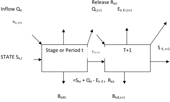
Now, given the initial storage volume Skt, the inflow Qit and the final storage volumes Sℓ,t+1 in period
‘t’, the releases Rkiℓt are determined by the continuity equation,
Rkiℓt = Skt + Qit - Ekℓt - Sℓ,t+1………(1)
Where Ekℓt is the possible evaporation and seepage loss based on the initial and final storage volumes
in period ‘t’.
It is clear from eqn.1 that the optimal reservoir releases Rkiℓt or equivalently the final storage volume
Sℓ,t+1 in each time period or stage depends on two state variables. The initial storage volume Skt and current
inflow Qit. Let Bkiℓt be the value of system performance associated with an initial reservoir storage volume of
‘Skt’, an inflow of Qot, a release of Rkiℓt, and a final volume of Sℓ,t+1 which is to be maximized and in the
objective of the Reservoir Operating problem. Recursive Equations:
To begin the development of the recursive backward moving DP algorithm, a particular period is selected after which it is assumed that the reservoir will no longer be operated. This can be any period in any year, because the eventual Steady state Reservoir Operating Policy derived from SDP Model will be independent of this arbitrary assumption provided that the valued of system performance Bkiℓt and transition
probabilities Pij do not change from one year to the next. Let, there are ‘t’ periods in a year and the objectives is
to maximize total annual benefits,
i.e maximize ∑ Bkiℓt
The sequential Reservoir operation process described as a multistage decision madding process is shown in fig.1 and the time periods for Reservoir operation is shown in fig.2
It can be noted form fig.1 that T+1 =1 as the cycle will be repeated in cyclic solution of recursive equations. Let the arbitrary terminal period be period ‘T’ now defining ft(k,i) as the total expected value of the
system performance with ‘n’ periods to go, including the current ‘t’ given that in period ‘t’ the initial storage volume and inflow are Skt and Qit respectively. Then with ony one period remaining
fT1 (k,i) = Max{ Bkiℓt} k,i ……….2
ℓ must be feasible given k,I, and t With two periods remaining before the end of Reservoir operation, the maximum expected value of system performance can be calculated as:
fT k, i ℓ pT fT ℓ, j ] k,i ………3
ℓ feasible where, is the probability of inflow Qj,T in period ‘T’ when the inflow in period T-1 equals Qi, T-1.
The function (k,i) is the expected system performance in the final two periods, since the inflow in period’T’ is not known with certainty in period T-1. The probability of any flow Qj,T in period ‘T’ depends on
the flow Qj, T-1 inperiod T-1, and is given by the transition probability . The recursive relationship, defined
by eqn 3 can be generalized as –
ℓ must be feasible where, ‘t’ refers to the within year period and ‘n’ to the total number of periods remaining before Reservoir operation terminates.
Steady State Operating Policy:
As these recursive equations are solved for each period in successive years, the policy ℓ (k,i,t) defined in each particular period ‘t’ will relatively quickly, repeat in each successive year. When this condition is satisfied, and when the expected annual performance, F T k, i F k, i , is constant for all states k,i and all periods ‘t’ within a year policy has reached a steady state.
Probability Distributions of Storage Volumes and Releases:
The steady state operating policy derived from the solution of the SDP Model defines the optimal final storage volume ‘S ℓ, t+1’. Let this policy be denoted by ℓ = ℓ (k,i,t). Assuming it as a ‘pure operating strategy’, the index
‘ℓ’ is not needed for the definition of the Reservoir releases and their joint probabilities. It can be specified by the policy ℓ= ℓ(k,i,t) for any value of k,i,t. thus the continuity equation can be written as
Rkit = Skt + Qit – Ekℓt – S ℓ, t+1 k,i ………..4
ℓ= ℓ(k,i,t)
and probability PRkit can be defined as the joint probability of the initial storage volume Skt the inflow and also
the final storage volume S ℓ, t+1,which is specified for each k,i,t by the function ℓ= ℓ(k,i,t) . Product of PRkit
with Ptij (stream flow transition probability) will give the joint results in the joint probability of S ℓ, t+1,and Qj,t+1
which can be denoted by PR ℓj, t+1.
i.e. PR ℓj, t+1 = ∑ PR * ……… ℓ,j,t ………….…5
ℓ= ℓ(k,i,t)
in addition, the joint probabilities, PRkit must sum to 1 in each time period ‘t’ i.e.
∑ PR = 1 t ………6
Simultaneous solution of the above set of equations 5, 6 will yield the values of PRkit. It can be observed that
one equation in 5 is redundant in each period ‘t’ and, the number of independent equations 5 and 6 equals the number of unknowns and thus a unique solution can be obtained. Knowing PRkit the corresponding marginal
probability distribution of Skt, Qit and Sℓ,t+1 associated with any operating policy ℓ= ℓ(k,i,t) can be obtained from
the following equations:
PSkt = ∑ PR k, t ………8
PQkt = ∑ PR i,t ………9
PS ℓ, t+1 = ∑ PR ℓ, t ………10
ℓ = ℓ (k,i,t) Reservoir Yield Function:
The results of releases obtained from the policy ℓ = ℓ (k,i,t) are arranged in descending order of their magnitude and corresponding values of PRkit are written against each value. Then cumulative probability is worked out for
Fig. Sequential Reservoir Operation Process
Results: The Probability which meeting out the demand of Ravishankar Sagar Reservoir:
Month Dependability Demand % Reliability of
satisfying Demand July 60% 65% 70% 75% 80% 85% 90% 138.4 138.4 138.4 138.4 138.4 138.4 138.4 0.95 0.86 0.80 0.80 0.75 0.70 0.70 August 60% 65% 70% 75% 80% 85% 90% 44.5 44.5 44.5 44.5 44.5 44.5 44.5 0.90 0.82 0.80 0.75 0.75 0.70 0.70 Sept. 60% 65% 70% 75% 80% 85% 90% 107.5 107.5 107.5 107.5 107.5 107.5 107.5 0.95 0.90 0.85 0.78 0.75 0.75 0.70 Oct. 60% 65% 70% 75% 80% 85% 90% 31.0 31.0 31.0 31.0 31.0 31.0 31.0 0.95 0.95 0.90 0.90 0.85 0.85 0.75 T+1 Stage or Period t
STATE Sk,t
Inflow Qit
Rki, t+1
Release Rkit Qi,t+1 Ek ℓ l,t+1
S ℓ, t+1
=Skt + Qit ‐ Ek ℓ t ‐ Rkit
Bkiℓt Bkiℓ,t+1
Storage Yield Functions for 75% Dependability Inflows:
Storage Yield functions for 90-% Dependability – values of Inflows:
Conclusions:
Based on the conducted study following major conclusions are made:
1. The values of % Reliability of meeting the demands in monsoon months can be evaluated considering various % dependability of monthly net Inflows from the developed Reservoir Yield Functions.
2. It has been observed that the demands in various months can be met with 75 – 90% reliability for different values of dependable net inflows.
3. The target storage values as obtained for various values of dependable net inflows can help the Managers of R.S.S. Reservoir to decide about the crop pattern in Rabi season
References:
[1] Buras N. (1985) “An application of mathematical programming in planning surface water storage”, water resources bulletin 21(6), pp 1013-1020.
[2] Yeh, W.M.G. (1985) “Reservoir Management and operation Models: State of Art Review. Water Resources Research, vol 21(2) pp 1797-1818.
[3] Shrivastava R.K. (1989) “ An on-line operation Model for Multi Reservoir Systems Ph.D. Thesis, IIT, Delhi, India. [4] Trivedi. M(1993) “ Operation Strategies for Optimal use of water Resources of Tawa Reservoir: A case Study.
[5] Cal.X.Mc.kinney.D. and Lasdon.L. (2001).” Solving nonlinear water management models using combined genetic and dynamic programming approach”. Adv. Water Resources 24(6), 667-676