University of Pennsylvania
ScholarlyCommons
Publicly Accessible Penn Dissertations
1-1-2016
Doubly Robust Causal Inference With Complex
Parameters
Edward Henry Kennedy
University of Pennsylvania, [email protected]
Follow this and additional works at:
http://repository.upenn.edu/edissertations
Part of the
Biostatistics Commons
This paper is posted at ScholarlyCommons.http://repository.upenn.edu/edissertations/1807
Recommended Citation
Kennedy, Edward Henry, "Doubly Robust Causal Inference With Complex Parameters" (2016).Publicly Accessible Penn Dissertations.
Doubly Robust Causal Inference With Complex Parameters
Abstract
Semiparametric doubly robust methods for causal inference help protect against bias due to model
misspecification, while also reducing sensitivity to the curse of dimensionality (e.g., when high-dimensional covariate adjustment is necessary). However, doubly robust methods have not yet been developed in numerous important settings. In particular, standard semiparametric theory mostly only considers independent and identically distributed samples and smooth parameters that can be estimated at classical root-n rates. In this dissertation we extend this theory and develop novel methodology for three settings outside these bounds: (1) matched cohort studies, (2) nonparametric dose-response estimation, and (3) complex high-dimensional effects with continuous instrumental variables. After giving an introduction in Chapter 1, we show in Chapter 2 that, for matched cohort studies, efficient and doubly robust estimators of effects on the treated are computationally equivalent to standard estimators that ignore the non-standard sampling. We also show that matched cohort studies are often more efficient than random sampling for estimating effects on the treated, and derive the optimal number of matches for given matching variables. We apply our methods in a study of the effect of hysterectomy on the risk of cardiovascular disease. In Chapter 3 we develop a novel approach for causal dose-response curve estimation that is doubly robust without requiring any parametric assumptions, and which naturally incorporates general off-the-shelf machine learning. We derive asymptotic properties for a kernel-based version of our approach and propose a data-driven method for bandwidth selection. The methods are used to study the effect of hospital nurse staffing on excess readmissions penalties. In Chapter 4 we develop novel estimators of the local instrumental variable curve, which represents the treatment effect among compliers who would take treatment when the instrument passes some threshold. Our methods do not require parametric assumptions, allow for flexible data-adaptive estimation of effect modification, and are doubly robust. We derive asymptotic properties under weak conditions, and use the methods to study infant mortality effects of neonatal intensive care units with high versus low technical capacity, using travel time as an instrument.
Degree Type Dissertation
Degree Name
Doctor of Philosophy (PhD)
Graduate Group
Epidemiology & Biostatistics
First Advisor Dylan S. Small
Keywords
Subject Categories
DOUBLY ROBUST CAUSAL INFERENCE WITH COMPLEX PARAMETERS
Edward H. Kennedy
A DISSERTATION
in
Epidemiology and Biostatistics
Presented to the Faculties of the University of Pennsylvania
in
Partial Fulfillment of the Requirements for the
Degree of Doctor of Philosophy
2016
Supervisor of Dissertation
Dylan S. Small, Professor of Statistics
Graduate Group Chairperson
John H. Holmes, Professor of Medical Informatics in Epidemiology
Dissertation Committee
Harold I. Feldman, Professor of Epidemiology & Medicine
DOUBLY ROBUST CAUSAL INFERENCE WITH COMPLEX PARAMETERS
c
COPYRIGHT
2016
Edward H. Kennedy
This work is licensed under the
Creative Commons Attribution
NonCommercial-ShareAlike 3.0
License
To view a copy of this license, visit
ACKNOWLEDGEMENT
To my advisors, Dylan and Marshall: I’m so grateful to have had the opportunity to work
with you over the last four years. You are two of the most intelligent, generous, and inspiring
people I’ve ever met, and I will always look up to you both.
Unfortunately I do not have enough space to appropriately thank everyone who contributed
to this dissertation work in some way. The long list includes:
– my dissertation committee (Eric, Harv, Taki, Zongming), who helped with everything
from moral support to administrative tasks to discussing proofs;
– the causal group (Alisa, Ashkan, Dylan, Jason, Jesse, Marshall, Peter, etc.), who
taught me a lot, generously listened to my ideas, and provided great discussions;
– many other faculty (Dick, Jason, Mary, Nandita, Peter, Taki, Zongming, etc.) who
selflessly shared their time and were excellent mentors and teachers;
– kind and supportive administrative staff (Cathy, Marissa, Noelle);
– fellow students at Penn and elsewhere (Bret, Emin, Jared, Julie, Jun, Valerio, etc.),
who kept my life balanced with good company, laughter, music, beer, and more.
I hope others who I have not listed by name still know how much I appreciate their help.
Lastly, I want to especially thank my family:
– To my brothers and sisters: You are all so important to me, and I would be lost
without you guys. Thank you for everything.
– To my parents: Your unwavering guidance and support has meant so much to me over
the years, and really made this work possible. I can’t say enough how much you have
inspired me, and how thankful I am for your faith in me.
– To Traci: Thank you for encouraging me, for being patient when I am in math mode,
ABSTRACT
DOUBLY ROBUST CAUSAL INFERENCE WITH COMPLEX PARAMETERS
Edward H. Kennedy
Dylan S. Small
Semiparametric doubly robust methods for causal inference help protect against bias due
to model misspecification, while also reducing sensitivity to the curse of dimensionality
(e.g., when high-dimensional covariate adjustment is necessary). However, doubly robust
methods have not yet been developed in numerous important settings. In particular,
stan-dard semiparametric theory mostly only considers independent and identically distributed
samples and smooth parameters that can be estimated at classical root-n rates. In this
dissertation we extend this theory and develop novel methodology for three settings outside
these bounds: (1) matched cohort studies, (2) nonparametric dose-response estimation, and
(3) complex high-dimensional effects with continuous instrumental variables. After giving
an introduction in Chapter 1, we show in Chapter 2 that, for matched cohort studies,
effi-cient and doubly robust estimators of effects on the treated are computationally equivalent
to standard estimators that ignore the non-standard sampling. We also show that matched
cohort studies are often more efficient than random sampling for estimating effects on the
treated, and derive the optimal number of matches for given matching variables. We apply
our methods in a study of the effect of hysterectomy on the risk of cardiovascular
dis-ease. In Chapter 3 we develop a novel approach for causal dose-response curve estimation
that is doubly robust without requiring any parametric assumptions, and which naturally
incorporates general off-the-shelf machine learning. We derive asymptotic properties for
a kernel-based version of our approach and propose a data-driven method for bandwidth
selection. The methods are used to study the effect of hospital nurse staffing on excess
readmissions penalties. In Chapter 4 we develop novel estimators of the local
treatment when the instrument passes some threshold. Our methods do not require
para-metric assumptions, allow for flexible data-adaptive estimation of effect modification, and
are doubly robust. We derive asymptotic properties under weak conditions, and use the
methods to study infant mortality effects of neonatal intensive care units with high versus
TABLE OF CONTENTS
ACKNOWLEDGEMENT . . . iv
ABSTRACT . . . v
LIST OF TABLES . . . x
LIST OF ILLUSTRATIONS . . . xi
CHAPTER 1 : INTRODUCTION . . . 1
CHAPTER 2 : SEMIPARAMETRIC CAUSAL INFERENCE IN MATCHED COHORT STUDIES . . . 3
2.1 Abstract . . . 3
2.2 Introduction . . . 3
2.3 Setup . . . 5
2.4 Identification and Estimation . . . 7
2.5 Efficiency and Design . . . 9
2.6 Simulations and Illustration . . . 12
CHAPTER 3 : NONPARAMETRIC METHODS FOR DOUBLY ROBUST ESTIMATION OF CONTINUOUS TREATMENT EFFECTS . . . 15
3.1 Abstract . . . 15
3.2 Introduction . . . 15
3.3 Background . . . 18
3.4 Main Results . . . 20
3.5 Simulation Study . . . 32
3.6 Application . . . 35
CHAPTER 4 : SEMIPARAMETRIC CAUSAL INFERENCE WITH
THE LOCAL INSTRUMENTAL VARIABLE CURVE . . . 40
4.1 Abstract . . . 40
4.2 Introduction . . . 40
4.3 Preliminaries . . . 44
4.4 Main Results . . . 49
4.5 Illustration . . . 62
4.6 Discussion . . . 67
APPENDIX TO CHAPTER 2 . . . 69
A.1 Brief Literature Review . . . 69
A.2 Effect Modification . . . 70
A.3 Proofs of identification and semiparametric theory . . . 71
A.4 Proofs of double robustness and asymptotics . . . 73
A.5 Proofs for Section 2.5 . . . 75
A.6 Additional Simulation Results . . . 77
A.7 Additional Illustration Details . . . 77
A.8 R Code . . . 79
APPENDIX TO CHAPTER 3 . . . 83
B.1 Guide to notation . . . 83
B.2 Proof of Theorem 3.1 . . . 84
B.3 Double robustness of efficient influence function & mapping . . . 86
B.4 TMLE version of estimator . . . 88
B.5 Stochastic equicontinuity lemmas . . . 89
B.6 Proof of Theorem 3.2 . . . 95
B.7 Proof of Theorem 3.3 . . . 103
B.8 Uniform consistency . . . 105
APPENDIX TO CHAPTER 4 . . . 109
C.1 Proof of Theorem 4.1 . . . 109
C.2 Proof of Theorem 4.2 . . . 110
C.3 Double robustness of efficient influence functionϕ . . . 114
C.4 Proof of Theorem 4.3 . . . 115
LIST OF TABLES
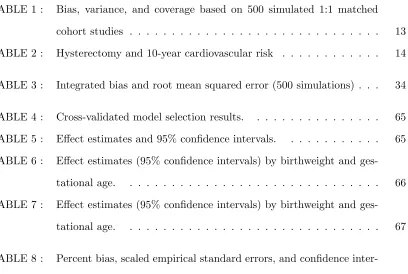
TABLE 1 : Bias, variance, and coverage based on 500 simulated 1:1 matched
cohort studies . . . 13
TABLE 2 : Hysterectomy and 10-year cardiovascular risk . . . 14
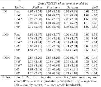
TABLE 3 : Integrated bias and root mean squared error (500 simulations) . . . 34
TABLE 4 : Cross-validated model selection results. . . 65
TABLE 5 : Effect estimates and 95% confidence intervals. . . 65
TABLE 6 : Effect estimates (95% confidence intervals) by birthweight and
ges-tational age. . . 66
TABLE 7 : Effect estimates (95% confidence intervals) by birthweight and
ges-tational age. . . 67
TABLE 8 : Percent bias, scaled empirical standard errors, and confidence
LIST OF ILLUSTRATIONS
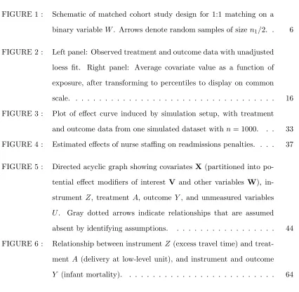
FIGURE 1 : Schematic of matched cohort study design for 1:1 matching on a
binary variableW. Arrows denote random samples of size n1/2. . 6
FIGURE 2 : Left panel: Observed treatment and outcome data with unadjusted
loess fit. Right panel: Average covariate value as a function of
exposure, after transforming to percentiles to display on common
scale. . . 16
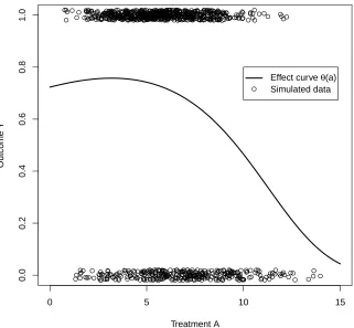
FIGURE 3 : Plot of effect curve induced by simulation setup, with treatment
and outcome data from one simulated dataset withn= 1000. . . 33
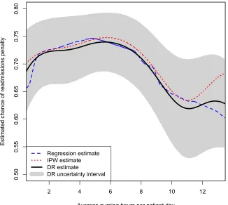
FIGURE 4 : Estimated effects of nurse staffing on readmissions penalties. . . . 37
FIGURE 5 : Directed acyclic graph showing covariatesX (partitioned into
po-tential effect modifiers of interest V and other variables W),
in-strument Z, treatment A, outcome Y, and unmeasured variables
U. Gray dotted arrows indicate relationships that are assumed
absent by identifying assumptions. . . 44
FIGURE 6 : Relationship between instrumentZ (excess travel time) and
treat-ment A (delivery at low-level unit), and instrument and outcome
CHAPTER 1 : INTRODUCTION
Many important problems in causal inference, missing data, and other settings lead to
pa-rameters that can be estimated doubly robustly. A full characterization of what it means
to be doubly robust and when exactly double robustness is possible is an open problem.
However, the following illustration covers many useful examples. Consider a target
pa-rameter ψ (e.g., an average treatment effect) and a corresponding estimator ˆψ, which is
constructed based on a sample of observed data (Z1, ..., Zn). Suppose further that ˆψ is a
regular asymptotically linear estimator with influence function ϕ, so that it has the
repre-sentation ˆψ = ψ0 +Pn{ϕ(Z)}+op(1/
√
n), where Pn denotes the empirical measure with
Pn(f) = n−1Pif(Zi), and Xn = op(rn) means Xn/rn converges in probability to zero.
Then the estimator ˆψ is doubly robust if the influence function ϕ(·) = ϕ(·;η) = ϕ(·;π, µ)
depends on two nuisance functions η = (π, µ) (e.g., a propensity score and outcome
re-gression function) and satisfies E{ϕ(Z;π0, µ)}=E{ϕ(Z;π, µ0)} =E{ϕ(Z;π0, µ0)} = 0 for
arbitrary η = (π, µ). Thus the influence function has mean zero (and thus is an unbiased
estimating function) as long as one of the two nuisance functions is evaluated at the truth.
Doubly robust estimators have several crucial advantages. First, they give analysts two
independent chances at arriving at the truth in large samples, since they are consistent
as long as only one of two nuisance functions is consistently estimated (i.e., even if one is
misspecified). This helps protect against bias from model misspecification, which is
partic-ularly important in complex high-dimensional data settings where simple parametric model
assumptions are unrealistic. Second, doubly robust estimators are also less sensitive to the
curse of dimensionality than more standard estimators. This follows from the fact that they
can attain faster rates of convergence than the nuisance estimators they depend on (when
both are consistently estimated); this is not the case for standard plug-in estimators, which
rely on a single nuisance estimator. Thus, even after model selection and machine
learning-based covariate adjustment, doubly robust estimators can yield fast rates of convergence
However, despite their many advantages and increasing popularity, doubly robust methods
have not yet been developed in numerous important settings. In particular, they have
mostly only been established for independent and identically distributed samples, and for
relatively straightforward target parameters that can be estimated at classical root-n rates
of convergence. In this dissertation we extend double robustness theory and develop novel
methodology for settings outside these bounds.
In Chapter 2 we consider semiparametric doubly robust estimation and inference in matched
cohort studies, which are a popular but non-standard sampling design. We show that
effi-cient doubly robust estimators of effects on the treated in such designs are computationally
equivalent to standard estimators that ignore the sampling, and explore various issues
re-lated to efficiency and study design. We apply our methods in a matched cohort study of
the effect of hysterectomy on the risk of cardiovascular disease. In Chapter 3 we develop
a novel nonparametric doubly robust approach for causal dose-response curve estimation,
which is an interesting but common example where double robustness is possible even
though standard root-n rates are not achievable. Our approach naturally incorporates
gen-eral off-the-shelf machine learning tools, and we explore its asymptotic properties under
weak conditions. We use our estimator to study the effect of hospital nurse staffing on
ex-cess readmissions penalties. Finally in Chapter 4 we develop novel semiparametric doubly
robust estimators of the local instrumental variable curve, which is a complex parameter
representing the treatment effect among compliers who would take treatment when the
instrument passes some threshold. We also develop an approach for doubly robust model
selection, and apply our methods to study the effects on infant mortality of delivery at
CHAPTER 2 : SEMIPARAMETRIC CAUSAL INFERENCE
IN MATCHED COHORT STUDIES
2.1. Abstract
Odds ratios can be estimated in case-control studies using standard logistic regression,
ignoring the outcome-dependent sampling. In this paper we discuss an analogous result
for treatment effects on the treated in matched cohort studies. Specifically, in studies
where a sample of treated subjects is observed along with a separate sample of possibly
matched controls, we show that efficient and doubly robust estimators of effects on the
treated are computationally equivalent to standard estimators, which ignore the matching
and exposure-based sampling. This is not the case for general average effects. We also show
that matched cohort studies are often more efficient than random sampling for estimating
effects on the treated, and derive the optimal number of matches for a given set of matching
variables. We illustrate our results via simulation and in a matched cohort study of the
effect of hysterectomy on the risk of cardiovascular disease.
2.2. Introduction
In this paper we consider matched cohort studies in which a sample of treated subjects
is observed along with a separate sample of possibly matched controls. Such studies are
particularly useful in settings where the treatment is relatively uncommon and it is expensive
to collect either the outcome data or the full set of covariates. These designs are also widely
used; according to PubMed the number of articles including both terms “matched” and
“cohort” has increased every year since 2000, and totals 19,581 as of 8 January 2015.
For example, Ingelsson et al. (2011) used a matched cohort design to estimate the effect
of hysterectomy on the risk of cardiovascular disease. They first identified all Swedish
women who underwent hysterectomies between 1973 and 2003 using the Swedish Inpatient
Register, and then for each of these women matched three additional women who did not
it was difficult to collect outcome data about cardiovascular events, as well as additional
covariate information such as socioeconomic status, because linkage to numerous additional
national health registers was required. More examples and general discussion of matched
cohort studies can be found in Jewell (2003) and Rothman et al. (2008).
Matched cohort studies are most often used for estimating treatment effects on the treated.
These effects can be of more interest than average effects, especially when treatment is
relatively rare and some subjects are very unlikely to receive it. A primary contribution of
this paper is to show that effects on the treated can be estimated in matched cohort studies
using standard methods, ignoring the study design; this is a cohort study analog of the
famous odds ratio result for case-control studies (Anderson, 1972; Prentice and Pyke, 1979).
To the best of our knowledge, this fact has never before been mentioned in the literature. It
means that, for example, even though propensity scores are not identified in matched cohort
designs, usual semiparametric, e.g., propensity score-based, doubly robust, estimators of the
effect on the treated can be applied without modification, and without requiring external
information about treatment prevalence or matched covariate distributions. Thus much of
the important literature on semiparametric estimation of effects on the treated (Heckman
et al., 1997; Hahn, 1998; Heckman et al., 1998; Hirano et al., 2003; Imbens, 2004; Abadie
and Imbens, 2006; Kline, 2011) is also relevant for matched cohort studies, even though this
work has mostly focused on simple random sampling.
A number of authors have considered causal inference in matched cohort study settings,
but none seem to have mentioned the above result. Heckman and Todd (2009) gave some
justification for using the propensity score in exposure-stratified studies without matching,
but did not discuss semiparametric theory or double robustness. Tchetgen Tchetgen and
Rotnitzky (2011) developed semiparametric theory and doubly robust estimators for the
conditional odds ratio but did not consider general marginal effects or efficiency across
study designs. Sj¨olander et al. (2012) and Sj¨olander and Greenland (2013) discussed using
Laan et al. (2013) examined cohort studies for community-based interventions, but required
external information beyond the sample.
2.3. Setup
We consider the following study setup. Covariates L and outcome Y are observed for n1
treated subjects along with n0 controls, where n0 = kn1 is fixed so that k controls are
selected for each treated subject. In addition the controls can be matched to the treated on
a subset of discrete covariatesW ⊆L. We use W =L\W to denote the set of covariates
not used in matching, so that L = (W, W). The observed data are (Z1, ..., Zn) with Z =
(L, A, Y) and A an indicator of treatment, where by design we have that P
iAi = n1,
P
i(1−Ai) = n0 = kn1, and Wi = Wj if subjects i and j are matched. If there is no
matching so thatW =∅and W =Lthen we simply observe two separate random samples
of treated and control subjects.
The main statistical issue in a matched cohort study is the fact that the observations are
not independent and identically distributed from the population of interest. Specifically,
the proportion treated in the sample is fixed due to the exposure-stratified sampling, and
the distribution of the matched covariates is forced to be the same for the treated and
control subjects due to the matching. Although the implications for causal inference are
different, this setup is conceptually similiar to that of a case-control study, where sampling
is stratified by outcome (Breslow et al., 2000). As in case-control studies, although the
observations in a matched cohort study are not an independent and identically distributed
sample from the population distribution of interest, they can be viewed as an independent
and identically distributed sample from a particular modified distribution. This is called the
biased sampling model framework (Jewell, 1985; Bickel et al., 1993). In a matched cohort
study the observations (Z1, ..., Zn) arise from a biased distribution Qwith density
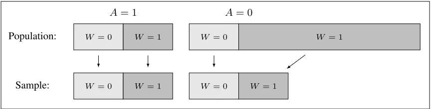
Population: W = 0 W = 1 A= 1
W = 0 W = 1 A= 0
Sample: W = 0 W = 1 W = 0 W = 1 (Note: arrows denote random samples of sizen1/2)
Population: W = 0 W = 1 A= 1
W = 0 W = 1 A= 0
Sample: W = 0 W = 1 W = 0 W = 1
3
Figure 1: Schematic of matched cohort study design for 1:1 matching on a binary variable W. Arrows denote random samples of size n1/2.
whereP denotes the distribution ofZ in a larger population of interest, with density given
by p(z) =p(y |l, a)p(l |a)p(a) with respect to some dominating measure, and q(a) is the
proportion of subjects in the sample receiving treatment level a. In general we write the
density under distribution F of variable X evaluated at value c asf(x= c), except when
the density we are referring to is unambiguous, e.g.,f(x) denotes the density ofXunderF.
The likelihood can be written as Q
ip(yi |li, ai)p(wi|wi, ai)q(ai)Qjp(wj |a= 1), wherei
references units andjreferences matched strata. For illustration Figure 1 gives a schematic
of a matched cohort study in the simple case of 1:1 matching on a binary variable.
In subsequent sections we characterize causal treatment effects using potential outcome
notation (Rubin, 1974), and so letYa denote the potential outcome that would have been
observed had treatment level a been applied. We further make use of some simplifying
notation. Specifically we useπ(l) to denote the propensity score underP given byp(a= 1|
l), and we use ξ(l) to denote the analog of the propensity score in the biased distribution
Qgiven by q(a= 1|l). We also useµ(l, a) to denote the conditional mean of the outcome
given covariates and treatmentE(Y |L=l, A=a), which is the same under bothP andQ
whenever it exists. All expectations are taken under the distribution P of interest, unless
2.4. Identification and Estimation
Throughout we consider the following identifying assumptions, the third of which is
com-monly called no unmeasured confounding.
Assumption 2.1 (Consistency) If A=athen Y =Ya with probability one.
Assumption 2.2 (Positivity) For all l such that p(l)>0, we have 0< π(l)<1.
Assumption 2.3 (Ignorability) Fora∈ {0,1}, E(Ya|L, A= 1) =E(Ya|L, A= 0).
These assumptions are all typically satisfied by design in randomized trials, but in
observa-tional studies they may be violated and are generally untestable. Consistency ensures that
one potential outcome is observed for every subject, namely that potential outcome under
the treatment that was actually received; it can fail to hold if different versions of treatment
have different effects, or if there is interference, for example. Positivity says that treatment
is not assigned deterministically, in the sense that every subject has some positive
probabil-ity of receiving both treatment and control, regardless of covariates. Ignorabilprobabil-ity says that
the mean potential outcomes are the same for both treatment groups once we condition on
the covariates, and requires sufficiently many relevant covariates to be collected.
It is well-known and straightforward to show that E(Ya) = R µ(l, a)p(l)dν(l) under
As-sumptions 2.1–2.3, whereν is a dominating measure for the distribution of L. Importantly,
his expression is identified under P, but not under Qsince we observeq(l)6=p(l) underQ.
Note that
p(l) =q(w|w, a= 0)p(w|a= 0)p(a= 0) +q(w|w, a= 1)q(w|a= 1)p(a= 1)
since q(w | w, a) = p(w | w, a) and q(w | a = 1) = p(w | a = 1), but at least p(a)
is not identified under Q. Without matching, the covariate distributions given treatment
distribution among the controls since it forces q(w | a = 0) = p(w | a = 1). Thus,
identification of average effects E(Ya) cannot be achieved under matched cohort sampling
without external knowledge of the treatment proportions p(a) and the matched covariate
densityp(w|a= 0).
Ifp(a) andp(w|a= 0) are known from external data, however, one can construct estimators
ofE(Ya), or any other parameter defined onP, based on appropriately weighted estimating
functions, as in van der Laan et al. (2013). Weighting is necessary since estimating functions
based on P will in general be biased, e.g., not have mean zero, under Q. For use in
matched cohort studies, estimating functions under P should be weighted by b(W, A) =
{p(A)/q(A)}{p(W |A)/p(W |a= 1)}sincep(z) =q(z)b(w, a).
In many cases such external information is not available, especially when W is
high-dimensional. But this is not problematic for estimation of the effect on the treated, which
is given by ψ=E(Y1−Y0|A= 1). Under Assumptions 2.1–2.3 we have
ψ= Z
y p(y|a= 1) dη(y)−
Z
µ(l,0)p(l|a= 1)dν(l),
where η is a dominating measure for the outcome distribution; this follows from the same
logic as in Hahn (1998) and elsewhere. Thus ψ is identified under Assumptions 2.1–2.3
in any study design that identifies p(y | l, a) and p(l | a = 1). Since these densities are
components of the density of distribution Q given in (2.1), it follows that ψ is identified
under matched cohort sampling.
As discussed by Breslow et al. (2000) in the context of case-control studies, this fact alone
also implies that influence functions for ψ under sampling from Q are equivalent to those
under sampling from P, but with densities under distribution Q replacing those under
P. For the sake of completeness, we follow Breslow et al. (2000) and prove this result
explicitly in the Appendix. To do so we use the same approach as Hahn (1998), with theory
detail elsewhere (Bickel et al., 1993; van der Laan and Robins, 2003; Tsiatis, 2006). The
result can also be derived by weighting the efficient influence function underP by the term
b(W, A) as discussed above.
Theorem 2.1 The efficient influence function for the effect on the treatedψ under a
non-parametric model with distribution Q is
ϕ(µ, ξ;ψ) = A q(a= 1)
n
Y −µ(L,0)−ψo− 1−A q(a= 1)
ξ(L) 1−ξ(L)
n
Y −µ(L,0)o.
A simple estimator based on the efficient influence function can be formulated by using the
efficient influence functionϕas an estimating function, after plugging in estimates ˆµ and ˆξ
of the nuisance functions, i.e., solvingQn{ϕ(ˆµ,ξˆ;ψ)}= 0 whereQnis the empirical measure
under Q. For example, ˆµ(l,0) could be predicted values from a regression of the outcome
on covariates using only control subjects, and ˆξ(l) could be predicted values from a logistic
regression of treatment on covariates. We show that this estimator is doubly robust and
derive its asymptotic properties in the Appendix.
Computationally, such estimators are exactly equivalent to those that would be used in a
simple study with standard random sampling. Thus, just as in case-control studies where
one can ignore the outcome-dependent sampling and regress outcome on exposure using
logistic regression to obtain valid odds ratio estimates, the above result justifies using
stan-dard estimators of effects on the treated in cohort studies with exposure-dependent sampling
and matching. In particular, one can use propensity score-based estimators as usual even
though the propensity score π(l) is not identified under matched cohort sampling. In the
Appendix we discuss estimation of effect modification among the treated.
2.5. Efficiency and Design
The semiparametric efficiency bound under sampling fromQis the variance of the efficient
in the Appendix that this efficiency bound can be expressed as
BQ=
Ω + Σ1
q(a= 1)+
p(a= 0) p(a= 1)
Σ∗0
q(a= 0), (2.2)
where Ω = var{µ(L,1)−µ(L,0) | A = 1}, Σ1 = E{σ2(L,1) | A = 1}, and Σ∗0 =
E{ς(W) | A = 0} with ς(w) = E[σ2(L,0)π(L)/{1−π(L)} | W = w, A = 1]. Letting
Σ0 =E[σ2(L,0)π(L)/{1−π(L)} |A = 1] =E{ς(W) |A = 1}, the efficiency bound under
P can be similarly expressed as BP = (Ω + Σ1+ Σ0)/p(a= 1).
The expressions for the bounds BQ and BP can simplify in certain cases; we will consider
three such settings here. The simplest is one in which there are no covariates, i.e., L=∅.
Then π(l) = p(a = 1) so that Σ∗0 = Σ0 = var(Y | A = 0)p(a = 1)/p(a = 0), and it also
follows that Ω = 0. Another setting of interest is when there are no matching variables, i.e.,
W = ∅. Then we again have Σ∗0 = Σ0, but without further simplification. Lastly we also
consider full matching, i.e., W =L. Then we have Σ∗0 = Σr
0, where Σr0 =E{σ2(L,0)p(a=
1)/p(a = 0) | A = 1} is the value of Σ0 we would see in a study had all subjects been
randomized to treatment with probabilityp(a= 1) regardless of covariates.
Using the above expressions for BQ andBP, it follows that BQ < BP if and only if
Σ∗0< q(a= 0) p(a= 0)
Σ0−
p(a= 1)−q(a= 1) q(a= 1)
Ω + Σ1
.
Clearly, there always exists a cohort study that can match the efficiency bound under
random sampling, since random sampling is equivalent to a cohort study with no matching
and with q(a = 1) = p(a = 1). In the next theorem we show the more interesting result
that there almost always exists a cohort study that is strictly more efficient than random
sampling.
Theorem 2.2 Suppose p(a = 1) 6= (Ω + Σ1)/(Ω + Σ1 + Σ0). Then there exists a cohort
efficiency bound strictly smaller than BP can be attained via an unmatched cohort study
with
min
p(a= 1), Ω + Σ1 Ω + Σ1+ Σ0
< q(a= 1)<max
p(a= 1), Ω + Σ1 Ω + Σ1+ Σ0
.
A proof of the above result is given in the Appendix. To illustrate, consider a simple cohort
study with no covariates and letσ2
a = var(Y |A=a). Then any cohort study with
p(a= 1)< q(a= 1)< p(a= 0)σ
2 1
p(a= 0)σ2
1 +p(a= 1)σ02
,
or the inequalities reversed, yields a smaller efficiency bound than random sampling. If
treatment is very rare or very common then nearly any cohort study will be more efficient
than random sampling, since then the condition approximates 0< q(a= 1)<1.
Matching can provide even more opportunities for efficiency gains. Consider two cohort
studies, one without matching, i.e., W = ∅, yielding efficiency bound Bu
Q and the other
fully matched, i.e.,W =L, yielding efficiency boundBm
Q. The difference between efficiency
bounds then equals
BuQ−BQm= 1 q(a= 0)
p(a= 0) p(a= 1)E
σ2(L,0)
π(L) 1−π(L) −
p(a= 1) p(a= 0)
A= 1
.
If there is no confounding so that π(l) = p(a = 1), then the bounds are clearly equal
and matching does not provide any efficiency gains. However, when there is confounding
the above will often be positive since π(l) will generally be larger than p(a = 1) among
the treated. For example, if σ2(l,0) is constant then Bu
Q ≥ Bqm by Jensen’s inequality.
This suggests that matched cohort studies will in general provide better efficiency than
unmatched cohort studies.
In principle one could design a fully efficient matched cohort study by minimizing the
matching variables W. Optimizing over different matching variables would be difficult in
practice, but results for optimizing overq(a= 1) are given in the following theorem.
Theorem 2.3 Consider a cohort study with a fixed set of (possibly empty) matching
vari-ables and given sample size. The optimal number of matches that maximizes efficiency for
estimation of ψ iskopt= [{p(a= 0)/p(a= 1)}{Σ∗0/(Ω + Σ1)}]1/2.
In the simplest matched cohort study with no covariates, this expression simplifies tokopt=
σ0/σ1. Thus for such studies the optimal matching ratio does not depend on the treatment
prevalence, and in particular 1:1 matching is optimal if the variance of the outcome is
constant across treatment groups. As intuition would suggest, if the variance of the outcome
is greater among controls then more matched controls should be used, and if the variance
is greater among the treated then fewer matched controls should be used.
2.6. Simulations and Illustration
2.6.1. Simulation Study
To explore finite-sample properties we adapt the simulation setup from Kang and Schafer
(2007). Specifically we simulated Lj ∼ N(0,1) for j = 1, ...,4, π(l) = expit(−1.7−l1+
0.5l2−0.25l3−0.1l4) so thatp(a= 1) = 0.20, andY =µ(L, A)+forµ(l, a) = 200+13.7l1+
13.7P
jlj + 10a, and ∼ N(0,1) so that ψ = 10. We generated matched cohort studies
with q(a= 1) = 0.5 and W =I(L1 >0), which ensures that q(a= 1 |l) follows a logistic
model with covariates w and l. For each simulated dataset we applied
inverse-probability-weighted, regression, and doubly robust estimators, with confidence intervals computed via
sandwich standard errors. To misspecify models we transformedL as in Kang and Schafer
(2007).
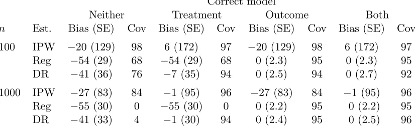
As shown in Table 1, the inverse-probability-weighted and regression estimators were biased
when relying on misspecified models, while the doubly robust estimator performed well as
Table 1: Bias, variance, and coverage based on 500 simulated 1:1 matched cohort studies
Correct model
Neither Treatment Outcome Both n Est. Bias (SE) Cov Bias (SE) Cov Bias (SE) Cov Bias (SE) Cov
100 IPW −20 (129) 98 6 (172) 97 −20 (129) 98 6 (172) 97 Reg −54 (29) 68 −54 (29) 68 0 (2.3) 95 0 (2.3) 95 DR −41 (36) 76 −7 (35) 94 0 (2.5) 94 0 (2.7) 92
1000 IPW −27 (83) 84 −1 (95) 96 −27 (83) 84 −1 (95) 96 Reg −55 (30) 0 −55 (30) 0 0 (2.2) 95 0 (2.2) 95 DR −41 (33) 4 −1 (30) 94 0 (2.4) 95 0 (2.5) 96
IPW, inverse probability weighted; Reg, regression; DR, doubly robust; n, sample size; SE, empirical standard error multiplied by n1/2; Cov, coverage (%).
similar efficiency when the outcome model was correct; when only the treatment model was
correct the doubly robust estimator was more efficient than the inverse-probability-weighted
estimator. Coverage was near 95% except under misspecification. In the Appendix we give
further results comparing with random sampling and different matching ratios.
2.6.2. Application
Here we analyze the 3:1 matched cohort study by Ingelsson et al. (2011) discussed in Section
2.2. We used the same three estimators as in the simulation study, with logistic regression
models for the treatment, i.e., hysterectomy, and outcome, i.e., cardiovascular disease within
10 years after enrollment. The matching covariates were birthyear and county of residence,
and the unmatched covariates were socioeconomic status and age at enrollment. For
simplic-ity we assumed independent censoring. As shown in Table 2, assuming no unmeasured
con-founding we estimate that hysterectomy yielded a statistically significant 0.55% increased
risk of cardiovascular disease within 10 years, among those who underwent hysterectomy.
We also used the formulas from Section 2.5 to analyze efficiency, by estimating the terms
in the bound BQ. For simplicity we assumed p(w | a) = p(w) and focused on varying
p(a). We estimate that 3:1 matched cohort sampling yields a smaller efficiency bound than
Table 2: Hysterectomy and 10-year cardiovascular risk
Method Estimate (%) SE (%) 95% CI p-value
IP-weighted 0.47 0.093 (0.29, 0.65) < 0.001 Regression 0.55 0.092 (0.37, 0.73) < 0.001 Doubly robust 0.55 0.092 (0.37, 0.73) < 0.001
CI, confidence interval; SE, standard error; IP, inverse-probability.
We also estimate that 3:1 matching is optimal if p(a = 1) = 3%, and that full matching
using socioeconomic status and age is beneficial if p(a= 1)<23%. More details are in the
CHAPTER 3 : NONPARAMETRIC METHODS FOR DOUBLY ROBUST
ESTIMATION OF CONTINUOUS TREATMENT EFFECTS
3.1. Abstract
Continuous treatments (e.g., doses) arise often in practice, but many available causal
ef-fect estimators are limited by either requiring parametric models for the efef-fect curve, or
by not allowing doubly robust covariate adjustment. We develop a novel kernel smoothing
approach that requires only mild smoothness assumptions on the effect curve, and still
al-lows for misspecification of either the treatment density or outcome regression. We derive
asymptotic properties and give a procedure for data-driven bandwidth selection. The
meth-ods are illustrated via simulation and in a study of the effect of nurse staffing on hospital
readmissions penalties.
3.2. Introduction
Continuous treatments or exposures (such as dose, duration, and frequency) arise very often
in practice, especially in observational studies. Importantly, such treatments lead to effects
that are naturally described by curves (e.g., dose-response curves) rather than scalars, as
might be the case for binary treatments. Two major methodological challenges in continuous
treatment settings are (1) to allow for flexible estimation of the dose-response curve (for
example to discover underlying structure without imposing a priori shape restrictions),
and (2) to properly adjust for high-dimensional confounders (i.e., pre-treatment covariates
related to treatment assignment and outcome).
Consider a recent example involving the Hospital Readmissions Reduction Program,
insti-tuted by the Centers for Medicare & Medicaid Services in 2012, which aimed to reduce
pre-ventable hospital readmissions by penalizing hospitals with excess readmissions. McHugh
et al. (2013) were interested in whether nurse staffing (measured in nurse hours per patient
data for 2976 hospitals, with nurse staffing (the ‘treatment’) on the x-axis, whether each
hospital was penalized (the outcome) on the y-axis, and a loess curve fit to the data
(with-out any adjustment). One way to characterize effects is to imagine setting all hospitals’
nurse staffing to the same level, and seeing if changes in this level yield changes in excess
readmissions risk. Such questions cannot be answered by simply comparing hospitals’ risk
of penalty across levels of nurse staffing, since hospitals differ in many important ways that
could be related to both nurse staffing and excess readmissions (e.g., size, location,
teach-ing status, among many other factors). The right panel of Figure 2 displays the extent of
these hospital differences, showing for example that hospitals with more nurse staffing are
also more likely to be high-technology hospitals and see patients with higher socioeconomic
status. To correctly estimate the effect curve, and fairly compare the risk of readmissions
penalty at different nurse staffing levels, one must adjust for hospital characteristics
appro-priately.
2 4 6 8 10 12
Average nursing hours per patient day
Chance of readmissions penalty
0
0.5
0.6
0.7
0.8
1
Observed data Unadjusted loess fit Uncertainty interval
2 4 6 8 10 12
0.3
0.4
0.5
0.6
0.7
0.8
Average nursing hours per patient day
A
v
er
age percentile r
ank
skilled nursing facility % Medicaid patients for profit status market competition % black patients urban location
teaching intensity number of beds operating margin % hispanic patients patient SES open−heart/transplant
Figure 2: Left panel: Observed treatment and outcome data with unadjusted loess fit. Right panel: Average covariate value as a function of exposure, after transforming to percentiles to display on common scale.
on regression modeling of how the outcome relates to covariates and treatment (e.g., Imbens
(2004), Hill (2011)). However, this approach relies entirely on correct specification of the
outcome model, does not incorporate available information about the treatment mechanism,
and is sensitive to the curse of dimensionality by inheriting the rate of convergence of the
outcome regression estimator. Hirano and Imbens (2004), Imai and van Dyk (2004), and
Galvao and Wang (2015) adapted propensity score-based approaches to the continuous
treatment setting, but these similarly rely on correct specification of at least a model for
treatment (e.g., the conditional treatment density).
In contrast, semiparametric doubly robust estimators (Robins and Rotnitzky, 2001; van der
Laan and Robins, 2003) are based on modeling both the treatment and outcome processes
and, remarkably, give consistent estimates of effects as long as one of these two nuisance
processes is modeled well enough (not necessarily both). Beyond giving two independent
chances at consistent estimation, doubly robust methods can also attain faster rates of
convergence than their nuisance (i.e., outcome and treatment process) estimators when
both models are consistently estimated; this makes them less sensitive to the curse of
dimensionality and can allow for inference even after using flexible machine learning-based
adjustment. However, standard semiparametric doubly robust methods for dose-response
estimation rely on parametric models for the effect curve, either by explicitly assuming
a parametric dose-response curve (Robins, 2000; van der Laan and Robins, 2003), or else
by projecting the true curve onto a parametric working model (Neugebauer and van der
Laan, 2007). Unfortunately, the first approach can lead to substantial bias under model
misspecification, and the second can be of limited practical use if the working model is far
away from the truth.
Recent work has extended semiparametric doubly robust methods to more complicated
nonparametric and high-dimensional settings. In a foundational paper, van der Laan and
Dudoit (2003) proposed a powerful cross-validation framework for estimator selection in
approach allows for global nonparametric modeling in general semiparametric settings
in-volving complex nuisance parameters. For example, D´ıaz and van der Laan (2013)
con-sidered global modeling in the dose-response curve setting, and developed a doubly robust
substitution estimator of risk. In nonparameric problems it is also important to consider
non-global learning methods, e.g., via local and penalized modeling (Gy¨orfi et al., 2002).
Rubin and van der Laan (2005, 2006a,b) proposed extensions to such paradigms in
nu-merous important problems, but the former considered weighted averages of dose-response
curves and the latter did not consider doubly robust estimation.
In this paper we present a new approach for causal dose-response estimation that is doubly
robust without requiring parametric assumptions, and which can naturally incorporate
gen-eral machine learning methods. The approach is motivated by semiparametric theory for a
particular stochastic intervention effect and a corresponding doubly robust mapping. Our
method has a simple two-stage implementation that is fast and easy to use with standard
software: in the first stage a pseudo-outcome is constructed based on the doubly robust
mapping, and in the second stage the pseudo-outcome is regressed on treatment via
off-the-shelf nonparametric regression and machine learning tools. We provide asymptotic results
for a kernel version of our approach under weak assumptions, which only require mild
smoothness conditions on the effect curve and allow for flexible data-adaptive estimation of
relevant nuisance functions. We also discuss a simple method for bandwidth selection based
on cross-validation. The methods are illustrated via simulation, and in the study discussed
earlier about the effect of hospital nurse staffing on excess readmission penalties.
3.3. Background
3.3.1. Data and notation
Suppose we observe an independent and identically distributed sample (Z1, ...,Zn) where
Z= (L, A, Y) has support Z = (L × A × Y). HereL denotes a vector of covariates, A a
effects using potential outcome notation (Rubin, 1974), and so letYa denote the potential
outcome that would have been observed under treatment levela.
We denote the distribution of Z by P, with density p(z) = p(y | l, a)p(a | l)p(l) with
respect to some dominating measure. We let Pn denote the empirical measure so that
empirical averages n−1P
if(Zi) can be written as Pn{f(Z)} = R
f(z)dPn(z). To simplify
the presentation we denote the mean outcome given covariates and treatment withµ(l, a) =
E(Y |L =l, A=a), denote the conditional treatment density given covariates with π(a|
l) = ∂a∂P(A ≤ a | L = l), and denote the marginal treatment density with $(a) =
∂
∂aP(A≤a). Finally, we use ||f||={ R
f(z)2dP(z)}1/2 to denote the L
2(P) norm, and we
use||f||X = supx∈X|f(x)|to denote the uniform norm of a generic functionf overx∈ X.
3.3.2. Identification
In this paper our goal is to estimate the effect curve θ(a) = E(Ya). Since this quantity
is defined in terms of potential outcomes that are not directly observed, we must consider
assumptions under which it can be expressed in terms of observed data. A full treatment of
identification in the presence of continuous random variables was given by Gill and Robins
(2001); we refer the reader there for details. The assumptions most commonly employed
for identification are as follows (the following must hold for any a∈ A at whichθ(a) is to
be identified).
Assumption 3.1 Consistency: A=aimplies Y =Ya.
Assumption 3.2 Positivity: π(a|l)≥πmin >0 for alll∈ L.
Assumption 3.3 Ignorability: E(Ya |L, A) =E(Ya|L).
Assumptions 3.1–3.3 can all be satisfied by design in randomized trials, but in observational
studies they may be violated and are generally untestable. The consistency assumption
en-sures that potential outcomes are defined uniquely by a subject’s own treatment level and
(i.e., no different versions of treatment). Positivity says that treatment is not assigned
deterministically, in the sense that every subject has some chance of receiving treatment
level a, regardless of covariates; this can be a particularly strong assumption with
contin-uous treatments. Ignorability says that the mean potential outcome under level a is the
same across treatment levels once we condition on covariates (i.e., treatment assignment is
unrelated to potential outcomes within strata of covariates), and requires sufficiently many
relevant covariates to be collected. Using the same logic as with discrete treatments, it
is straightforward to show that under Assumptions 3.1–3.3 the effect curve θ(a) can be
identified with observed data as
θ(a) =E{µ(L, a)}=
Z
L
µ(l, a)dP(l). (3.1)
Even if we are not willing to rely on Assumptions 3.1 and 3.3, it may often still be of interest
to estimateθ(a) as an adjusted measure of association, defined purely in terms of observed
data.
3.4. Main Results
In this section we develop doubly robust estimators of the effect curveθ(a) without relying
on parametric models. First we describe the logic behind our proposed approach, which is
based on finding a doubly robust mapping whose conditional expectation given treatment
equals the effect curve of interest, as long as one of two nuisance parameters is correctly
specified. To find this mapping, we derive a novel efficient influence function for a stochastic
intervention parameter. Our proposed method is based on regressing this doubly robust
mapping on treatment using off-the-shelf nonparametric regression and machine learning
methods. We derive asymptotic properties for a particular version of this approach based
on local-linear kernel smoothing. Specifically, we give conditions for consistency and
asymp-totic normality, and describe how to use cross-validation to select the bandwidth parameter
3.4.1. Setup and doubly robust mapping
Ifθ(a) is assumed known up to a finite-dimensional parameter, for exampleθ(a) =ψ0+ψ1a
for (ψ0, ψ1)∈R2, then standard semiparametric theory can be used to derive the efficient
influence function, from which one can obtain the efficiency bound and an efficient estimator
(Bickel et al., 1993; van der Laan and Robins, 2003; Tsiatis, 2006). However, such theory is
not directly available if we only assume, for example, mild smoothness conditions on θ(a)
(e.g., differentiability). This is due to the fact that without parametric assumptions θ(a)
is not pathwise differentiable, and root-n consistent estimators do not exist (Bickel et al.,
1993; D´ıaz and van der Laan, 2013). In this case there is no developed efficiency theory.
To derive doubly robust estimators forθ(a) without relying on parametric models, we adapt
semiparametric theory in a novel way similar to the approach of Rubin and van der Laan
(2005, 2006a). Our goal is to find a functionξ(Z;π, µ) of the observed dataZand nuisance
functions (π, µ) such that
E{ξ(Z;π, µ)|A=a}=θ(a)
if either π = π or µ = µ (not necessarily both). Given such a mapping, off-the-shelf
nonparametric regression and machine learning methods could be used to estimateθ(a) by
regressing ξ(Z; ˆπ,µˆ) on treatmentA, based on estimates ˆπ and ˆµ.
This doubly robust mapping is intimately related to semiparametric theory and especially
the efficient influence function for a particular parameter. Specifically, ifE{ξ(Z;π, µ)|A=
a}=θ(a) then it follows thatE{ξ(Z;π, µ)}=ψ for
ψ= Z
A
Z
L
µ(l, a)$(a) dP(l)da. (3.2)
This indicates that a natural candidate for the unknown mapping ξ(Z;π, µ) would be a
component of the efficient influence function for the parameter ψ, since for regular
φ(Z;π, µ) will be doubly robust in the sense that E{φ(Z;π, µ)} = 0, if either π = π
or µ = µ (Robins and Rotnitzky, 2001; van der Laan and Robins, 2003). This implies
E{φ(Z;π, µ)} =E{ξ(Z;π, µ)−ψ}= 0 so that E{ξ(Z;π, µ)}=ψ if either π =π orµ=µ.
This kind of logic was first used by Rubin and van der Laan (2005, 2006a) for full data
pa-rameters that are functions of covariates rather than treatment (i.e., censoring) variables.
The parameterψ is also of interest in its own right. In particular, it represents the average
outcome under an intervention that randomly assigns treatment based on the density $
(i.e., a randomized trial). Thus comparing the value of this parameter to the average
observed outcome provides a test of treatment effect; if the values differ significantly, then
there is evidence that the observational treatment mechanism impacts outcomes for at least
some units. Stochastic interventions were discussed by D´ıaz and van der Laan (2012),
for example, but the efficient influence function for ψ has not been given before under a
nonparametric model. Thus in Theorem 3.1 below we give the efficient influence function
for this parameter respecting the fact that the marginal density $is unknown.
Theorem 3.1 Under a nonparametric model, the efficient influence function forψ defined
in (3.2) isξ(Z;π, µ)−ψ+R
A{µ(L, a)−
R
Lµ(l, a)dP(l)}$(a)da, where
ξ(Z;π, µ) = Y −µ(L, A) π(A|L)
Z
L
π(A|l) dP(l) + Z
L
µ(l, A) dP(l).
A proof of Theorem 3.1 is given in the Appendix. Importantly, we also prove that the
function ξ(Z;π, µ) satisfies its desired double robustness property, i.e., that E{ξ(Z;π, µ) |
A = a} = θ(a) if either π =π or µ =µ. As mentioned earlier, this motivates estimating
the effect curve θ(a) by estimating the nuisance functions (π, µ), and then regressing the
estimated pseudo-outcome
ˆ
ξ(Z; ˆπ,µˆ) = Y −µˆ(L, A) ˆ
π(A|L) Z
L
ˆ
π(A|l) dPn(l) + Z
L
ˆ
on treatment A using off-the-shelf nonparametric regression or machine learning methods.
In the next subsection we describe our proposed approach in more detail, and analyze the
properties of an estimator based on kernel estimation.
3.4.2. Proposed Approach
In the previous subsection we derived a doubly robust mappingξ(Z;π, µ) for whichE{ξ(Z;π, µ)|
A=a}=θ(a) as long as eitherπ=πorµ=µ. This indicates that doubly robust
nonpara-metric estimation ofθ(a) can proceed with a simple two-step procedure, where both steps
can be accomplished with flexible machine learning. To summarize, our proposed method
is:
1. Estimate nuisance functions (π, µ) and obtain predicted values.
2. Construct pseudo-outcome ˆξ(Z; ˆπ,µˆ) and regress on treatment variableA.
We give sample code implementing the above in the Appendix.
In what follows we present results for an estimator that uses kernel smoothing in Step 2.
Such an approach is related to kernel approximation of a full-data parameter in censored
data settings. Robins and Rotnitzky (2001) gave general discussion and considered density
estimation with missing data, while van der Laan and Robins (1998), van der Laan and Yu
(2001), and van der Vaart and van der Laan (2006) used the approach for current status
survival analysis; Wang et al. (2010) used it implicitly for nonparametric regression with
missing outcomes.
As indicated above, however, a wide variety of flexible methods could be used in our Step 2,
including local partitioning or nearest neighbor estimation, global series or spline methods
with complexity penalties, or cross-validation-based combinations of methods, e.g., Super
Learner (van der Laan et al., 2007). In general we expect the results we report in this paper
to hold for many such methods. To see why, let ˆθdenote the proposed estimator described
in Step 2), and letθdenote an estimator based on an oracle version of the pseudo-outcome
ξ(Z;π, µ) where (π, µ) are the unknown limits to which the estimators (ˆπ,µˆ) converge. Then
||θˆ−θ|| ≤ ||θˆ−θ||+||θ−θ||, where the second term on the right can be analyzed with
standard theory since θ is a regression of a simple fixed function ξ(Z;π, µ) on A, and the
first term will be small depending on the convergence rates of ˆπ and ˆµ. A similar point was
discussed by Rubin and van der Laan (2005, 2006a).
The local linear kernel version of our estimator is ˆθh(a) = gha(a)Tβˆh(a), where gha(t) =
(1,t−ha)T and
ˆ
βh(a) = arg min β∈R2
Pn
Kha(A) n
ˆ
ξ(Z; ˆπ,µˆ)−gha(A)Tβ o2
(3.3)
forKha(t) =h−1K{(t−a)/h} withK a standard kernel function (e.g., a symmetric
prob-ability density) andh a scalar bandwidth parameter. This is a standard local linear kernel
regression of ˆξ(Z; ˆπ,µˆ) on A. For overviews of kernel smoothing see, e.g., Fan and Gijbels
(1996), Wasserman (2006), and Li and Racine (2007). Under near-violations of positivity,
the above estimator could potentially lie outside the range of possible values for θ(a) (e.g.,
if Y is binary); thus we present a targeted minimum loss-based estimator (TMLE) in the
Appendix, which does not have this problem. Alternatively one could project onto a logistic
model in (3.3).
3.4.3. Consistency of Kernel Estimator
In Theorem 3.2 below we give conditions under which the proposed kernel estimator ˆθh(a)
is consistent for θ(a), and also give the corresponding rate of convergence. In general this
result follows if the bandwidth decreases with sample size slowly enough, and if either of
the nuisance functionsπ orµ is estimated well enough (not necessarily both). The rate of
convergence is a sum of two rates: one from standard nonparametric regression problems
(depending on the bandwidth h), and another coming from estimation of the nuisance
Theorem 3.2 Let π and µdenote fixed functions to which πˆ and µˆ converge in the sense
that||πˆ−π||Z =op(1)and||µˆ−µ||Z =op(1), and let a∈ Adenote a point in the interior of
the compact supportA ofA. Along with Assumption 3.2 (Positivity), assume the following:
1. Either π =π or µ=µ.
2. The bandwidth h=hn satisfiesh→0 and nh3 → ∞ as n→ ∞.
3. K is a continuous symmetric probability density with support [−1,1].
4. θ(a) is twice continuously differentiable, and both$(a) and the conditional density of
ξ(Z;π, µ) given A=aare continuous as functions of a.
5. The estimators (ˆπ,µˆ) and their limits(π, µ) are contained in uniformly bounded
func-tion classes with finite uniform entropy integrals (as defined in the Appendix), with
1/πˆ and 1/π also uniformly bounded.
Then
|θˆh(a)−θ(a)|=Op
1
√ nh+h
2+r
n(a)sn(a)
where
sup t:|t−a|≤h
||πˆ(t|L)−π(t|L)||=Op
r(n)
sup t:|t−a|≤h
||µˆ(L, t)−µ(L, t)||=Op
s(n)
are the ‘local’ rates of convergence of πˆ andµˆ near A=a.
A proof of Theorem 3.2 is given in the Appendix. The required conditions are all quite weak.
Condition (a) is arguably the most important of the conditions, and says that at least one
of the estimators ˆπor ˆµmust be consistent for the trueπorµin terms of the uniform norm.
Since only one of the nuisance estimators is required to be consistent (not both), Theorem
3.2 shows the double robustness of the proposed estimator ˆθh(a). Conditions (b), (c), and
involves the complexity of the estimators ˆπ and ˆµ(and their limits), and is a usual minimal
regularity condition for problems involving nuisance functions.
Condition (b) says that the bandwidth parameter h decreases with sample size but not
too quickly (so that nh3 → ∞). This is a standard requirement in local linear kernel
smoothing (Fan and Gijbels, 1996; Wasserman, 2006; Li and Racine, 2007). Note that since
nh = nh3/h2, it is implied that nh → ∞; thus one can view nh as a kind of effective
or local sample size. Roughly speaking, the bandwidth h needs to go to zero in order to
control bias, while the local sample size nh (and nh3) needs to go to infinity in order to
control variance. We postpone more detailed discussion of the bandwidth parameter until
a later subsection, where we detail how it can be chosen in practice using cross-validation.
Condition (c) puts some minimal restrictions on the kernel function. It is clearly satisfied for
most common kernels, including the uniform kernelK(u) =I(|u| ≤1)/2, the Epanechnikov
kernel K(u) = (3/4)(1−u2)I(|u| ≤ 1), and a truncated version of the Gaussian kernel
K(u) =I(|u| ≤1)φ(u)/{2Φ(1)−1}withφand Φ the density and distribution functions for a
standard normal random variable. Condition (d) restricts the smoothness of the effect curve
θ(a), the density of $(a), and the conditional density given A=a of the limiting
pseudo-outcome ξ(Z;π, µ). These are standard smoothness conditions imposed in nonparametric
regression problems. By assuming more smoothness of θ(a), bias-reducing (higher-order)
kernels could achieve faster rates of convergence and even approach the parametric root-n
rate (see for example Fan and Gijbels (1996), Wasserman (2006), and others).
Condition (e) puts a mild restriction on how flexible the nuisance estimators (and their
corresponding limits) can be, although such uniform entropy conditions still allow for a wide
array of data-adaptive estimators and, importantly, do not require the use of parametric
models. Andrews (1994) (Section 4), van der Vaart and Wellner (1996) (Sections 2.6–2.7),
and van der Vaart (2000) (Examples 19.6–19.12) discuss a wide variety of function classes
with finite uniform entropy integrals. Examples include standard parametric classes of
condition), smooth functions with uniformly bounded partial derivatives, Sobolev classes of
functions, as well as convex combinations or Lipschitz transformations of any such sets of
functions. The uniform entropy restriction in condition (e) is therefore not a very strong
restriction in practice; however, it could be further weakened via sample splitting techniques
(see Chapter 27 of van der Laan and Rose (2011)).
The convergence rate given in the result of Theorem 3.2 is a sum of two components.
The first, 1/√nh+h2, is the rate achieved in standard nonparametric regression problems
without nuisance functions. Note that if h tends to zero slowly, then 1/√nh will tend
to zero quickly but h2 will tend to zero more slowly; similarly if h tends to zero quickly,
then h2 will as well, but 1/√nh will tend to zero more slowly. Balancing these two terms
requires h ∼ n−1/5 so that 1/√nh ∼ h2 ∼ n−2/5. This is the optimal pointwise rate
of convergence for standard nonparametric regression on a single covariate, for a twice
continuously differentiable regression function.
The second component,rn(a)sn(a), is the product of the local rates of convergence (around
A = a) of the nuisance estimators ˆπ and ˆµ towards their targets π and µ. Thus if the
nuisance function estimates converge slowly (due to the curse of dimensionality), then the
convergence rate of ˆθh(a) will also be slow. However, since the term is a product, we
have two chances at obtaining fast convergence rates, showing the bias-reducing benefit of
doubly robust estimators. The usual explanation of double robustness is that, even if ˆµ is
misspecified so thatsn(a) =O(1), then as long as ˆπ is consistent, i.e.,rn(a) =o(1), we will
still have consistency since rn(a)sn(a) =o(1). But this idea also extends to settings when
both ˆπ and ˆµare consistent. For example supposeh∼n−1/5 so that 1/√nh+h2 ∼n−2/5,
and suppose ˆπ and ˆµ are locally consistent with rates rn(a) = n−2/5 and sn(a) = n−1/10.
Then the product is rn(a)sn(a) = O(n−1/2) = o(n−2/5) and the contribution from the
nuisance functions is asymptotically negligible, in the sense that the proposed estimator
has the same convergence rate as an infeasible estimator with known nuisance functions.
matches that of the nuisance function estimator, rather than being faster (van der Vaart,
2014).
In the Appendix we give some discussion of uniform consistency, which, along with weak
convergence, will be pursued in more detail in future work.
3.4.4. Asymptotic Normality of Kernel Estimator
In the next theorem we show that if one or both of the nuisance functions are estimated at
fast enough rates, then the proposed estimator is asymptotically normal after appropriate
scaling.
Theorem 3.3 Consider the same setting as Theorem 3.2. Along with Assumption 3.2
(Positivity) and conditions (a)–(e) from Theorem 3.2, also assume that:
(f ) The local convergence rates satisfy rn(a)sn(a) =op(1/
√ nh).
Then
√
nhnθˆh(a)−θ(a) +bh(a) o
N
0, σ
2(a)R
K(u)2 du
$(a)
where bh(a) =θ00(a)(h2/2) R
u2K(u) du+o(h2), and
σ2(a) =E
τ2(L, a) +{µ(L, a)−µ(L, a)}2
{π(a|L)/$(a)}2/{π(a|L)/$(a)}
−nθ(a)−m(a)o2
for τ2(l, a) =var(Y |L=l, A=a),$(a) =
E{π(a|L)}, m(a) =E{µ(L, a)}.
The proof of Theorem 3.3 is given in the Appendix. Conditions (a)–(e) are the same as
in Theorem 3.2 and were discussed earlier. Condition (f) puts a restriction on the local
convergence rates of the nuisance estimators. This will in general require at least some
semiparametric modeling of the nuisance functions. Truly nonparametric estimators of π
and µ will typically converge at slow rates due to the curse of dimensionality, and will
covari-asymptotically; depending on the specific nuisance estimators used, it could be possible
to give weaker but more complicated conditions that allow for a non-negligible asymptotic
contribution while still yielding asymptotic normality.
Importantly, the rate of convergence required by condition (g) of Theorem 3.3 is slower than
the root-n rate typically required in standard semiparametric settings where the parameter
of interest is finite-dimensional and Euclidean. For example, in a standard setting where the
support A is finite, a sufficient condition for yielding the requisite asymptotic negligibility
for attaining efficiency isrn(a) =sn(a) =o(n−1/4); however in our setting the weaker
con-ditionrn(a) =sn(a) =o(n−1/5) would be sufficient if h∼n−1/5. Similarly, if one nuisance
estimator ˆπor ˆµis computed with a correctly specified generalized additive model, then the
other nuisance estimator would ony need to be consistent (without a rate condition). This
is because, under regularity conditions and with optimal smoothing, a generalized additive
model estimator converges at rate Op(n−2/5) (Horowitz, 2009), so that if the other
nui-sance estimator is merely consistent we havern(a)sn(a) =O(n−2/5)o(1) =o(n−2/5), which
satisfies condition (f) as long ash∼n−1/5. In standard settings such flexible nuisance
esti-mation would make a non-negligible contribution to the limiting behavior of the estimator,
preventing asymptotic normality and root-n consistency.
Under the assumptions of Theorem 3.3, the proposed estimator is asymptotically normal
after appropriate scaling and centering. However, the scaling is by the square root of the
local sample size √nh rather than the usual parametric rate√n. This slower convergence
rate is a cost of making fewer assumptions (equivalently, the cost of better efficiency would
be less robustness); thus we have a typical bias-variance trade-off. As in standard
non-parametric regression, the estimator is consistent but not quite centered atθ(a); there is a
bias term of order O(h2), denoted b
h(a). In fact the estimator is centered at a smoothed
version of the effect curveθ∗
h(a) =gha(a)Tβh(a) =θ(a) +bh(a). This phenomenon is
ubiq-uitous in nonparametric regression, and complicates the process of computing confidence