A Novel Class Imbalance Learning Method using Neural Networks

A Novel Class Imbalance Learning Method using Neural

Networks

K. Nageswara Rao

Research Scholar, GITAM University,

Visakhapatnam. Andhra Pradesh, India

D. Rajya Lakshmi

Phd, Prof,Dept of IT,GITAM University

Visakapatnam.Andhra Pradesh,India

T. Venkateswara Rao

Prof, Dept of CSE, KL University Vijayawada,Andhra Pradesh,India

.

ABSTRACT

In Data mining and Knowledge Discovery hidden and valuable knowledge from the data sources is discovered. The traditional algorithms used for knowledge discovery are bottle necked due to wide range of data sources availability. Class imbalance is a one of the problem arises due to data source which provide unequal class i.e. examples of one class in a training data set vastly outnumber examples of the other class(es). In this paper, we present a new hybrid approach using neural networks to improve the class imbalance results. This algorithm provides a simpler and faster alternative by using multi perceptron back propagation neural network as base algorithm. We conduct experiments using eleven UCI data sets from various application domains using four base learners, and five evaluation metrics. Experimental results show that our method has shown good performance in terms of Area under the ROC Curve, F-measure, precision, TP rate and TN rate values than many existing class imbalance learning methods.

Index Terms

1. INTRODUCTION

A dataset is class imbalanced if the classification categories are not approximately equally represented. The level of imbalance (ratio of size of the majority class to minority class) can be as huge as 1:99[1]. It is noteworthy that class imbalance is emerging as an important issue in designing classifiers [2], [3], [4]. Furthermore, the class with the lowest number of instances is usually the class of interest from the point of view of the learning task [5]. This problem is of great interest because it turns up in many real-world classification problems, such as remote-sensing [6], pollution detection [7], risk management [8], fraud detection [9], and especially medical diagnosis [10]–[13]. There exist techniques to develop better performing classifiers with imbalanced datasets, which are generally called Class Imbalance Learning (CIL) methods. These methods can be broadly divided into two categories, namely, external methods and internal methods. External methods involve preprocessing of training datasets in order to make them balanced, while internal methods deal with modifications of the learning algorithms in order to reduce their sensitiveness to class imbalance [14]. The main advantage of external methods as previously pointed out, is that they are independent of the underlying classifier. In this paper, we are laying more stress to propose an external CIL method for solving the class imbalance problem.

This paper is organized as follows. Section 2 briefly reviews the Data Balancing problems and its measures. And in Section 3, we discuss the proposed method of using the back propagation neural network as one of the component for CIL. Section 4 presents the imbalanced datasets used and measures used for validation, while In Section 5, we present the experimental setting and In Section 6discuss, in detail, the classification

results obtained by the proposed method and compare them with the results obtained by different existing methods and finally, in Section 7, we conclude the paper.

2. DATA BALANCING

Whenever a class in a classification task is underrepresented (i.e., has a lower prior probability) compared to other classes, we consider the data as imbalanced [15], [16]. The main problem in imbalanced data is that the majority classes that are represented by large numbers of patterns rule the classifier decision boundaries at the expense of the minority classes that are represented by small numbers of patterns. This leads to high and low accuracies in classifying the majority and minority classes, respectively, which do not necessarily reflect the true difficulty in classifying these classes. Most common solutions to this problem balance the number of patterns in the minority or majority classes.

Either way, balancing the data has been found to alleviate the problem of imbalanced data and enhance accuracy [15],[16], [17]. Data balancing is performed by, e.g., oversampling patterns of minority classes either randomly or from areas close to the decision boundaries. Interestingly, random oversampling is found comparable to more sophisticated oversampling methods [17]. Alternatively, under sampling is performed on majority classes either randomly or from areas far away from the decision boundaries. We note that random under sampling may remove significant patterns and random oversampling may lead to over fitting, so random sampling should be performed with care. We also note that, usually, oversampling of minority classes is more accurate than under sampling of majority classes [17].

Resampling techniques can be categorized into three groups. Under sampling methods, which create a subset of the original data-set by eliminating instances (usually majority class instances); oversampling methods, which create a superset of the original data-set by replicating some instances or creating new instances from existing ones; and finally, hybrids methods that combine both sampling methods. Among these categories, there exist several different proposals; from this point, we only center our attention in those that have been used in under sampling.

 Random under sampling: It is a non heuristic method that aims to balance class distribution through the random elimination of majority class examples. Its major drawback is that it can discard potentially useful data, which could be important for the induction process.

 Random oversampling: In the same way as random

 Hybrid Methods: In this hybrid method both under sampling and oversampling will be applied for the datasets so as to make it a balance dataset.

The bottom line is that when studying problems with imbalanced data, using the classifiers produced by standard machine learning algorithms without adjusting the output threshold may well be a critical mistake. This skewness towards minority class (positive) generally causes the generation of a high number of false-negative predictions, which lower the model’s performance on the positive class compared with the performance on the negative (majority) class. A comprehensive review of different CIL methods can be found in [18]. The following two sections briefly discuss the external-imbalance and internal-imbalance learning methods.

The external methods are independent from the learning algorithm being used, and they involve preprocessing of the training datasets to balance them before training the classifiers. Different resampling methods, such as random and focused oversampling and under sampling, fall into to this category. In random under sampling, the majority-class examples are removed randomly, until a particular class ratio is met [19]. In random oversampling, the minority-class examples are randomly duplicated, until a particular class ratio is met [18]. Synthetic minority oversampling technique (SMOTE) [20] is an oversampling method, where new synthetic examples are generated in the neighborhood of the existing minority-class examples rather than directly duplicating them. In addition, several informed sampling methods have been introduced in [21]. A clustering-based sampling method has been proposed in [22], while a genetic algorithm based sampling method has been proposed in [23].

3. CLASS IMBALANCE LEARNING

USING SUBSET FILTERI

In this section, we follow a design decomposition approach to systematically analyze the different unbalanced domains. We first briefly introduce the design decomposition methodology adopted for new proposed approach.

Algorithm 1:CIL-NN

1: {Input: A set of minor class examples P, a set

Of major class examples N,jPj<jN j, and T,

The number of subsets to be sampled from N.}

2: i ← 0, T=N/P.

3: repeat

4: i= i+ 1

5: Randomly sample a subset Ni from N,

jNij=jPj.

6: Combine P and Ni to form NPi

6: Apply filter on a NPi

7: Train and Learn A Base Classifier (BPN)

Using NPi. Obtain the values of

AUC,TP,FP,F-Measure

7: until i= T

8: Output: Average Measure;

The different components of our proposed algorithm are elaborated in the next subsections.

3.1 Dataset Sampling

An easy way to sample a dataset is by selecting instances randomly from all classes. However, sampling in this way can break the dataset in an unequal priority way and more number of instances of the same class may be chosen in sampling. To resolve this problem and maintain uniformity in sample, we propose a sampling strategy called weighted component sampling. Before creating multiple subsets, we will create the number of majority subsets depending upon the number of minority instances.

3.2 Identifying number of subsets of majority

class

The ratio of majority and minority instances in the unbalanced dataset is used to decide the number of subset of majority instances (T) to be created.

T= no. of majority inst(N)./no. of minority inst(P).

3.3 Applying filter

Subsets of majority instances are combined with minority subset and multiple balanced subsets are formed. Applying a specific filtering technique at this stage will help to reduce the class imbalance effects. So, Correlation based Feature Subset (CFS) filter is applied at this stage.

3.4. Averaging the measures

The subsets of balanced datasets created are used to run multiple times and the resulted values are averaged to find the overall result. In results we have obtained observations for AUC, Precision, F-measure, Sensitivity, Specificity and Accuracy by using Back Propagation Neural Networks as its base classifier.

4. DATASETS AND MEASURES

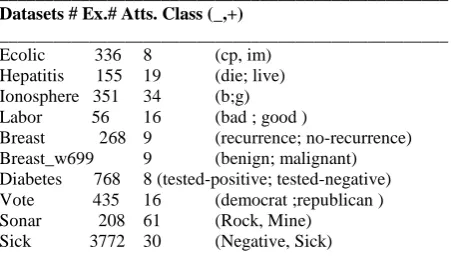
We considered four benchmark real-world imbalanced dataset from the UCI machine learning repository [24] to validate our proposed method. Table II summarizes the details of these datasets in the ascending order of the positive-to-negative dataset ratio. This contains the name of the dataset, the total number of examples (Total), attribute, the number of target classes for each dataset, number of minority class examples (#min.), the number of .majority class examples (#maj.). These datasets represent a whole variety of domains, complexities, and imbalance ratios.

For every data set, we perform a tenfold stratified cross validation. Within each fold, the classification method is repeated ten times considering that the sampling of subsets introduces randomness. The AUC, Precision, F-measure, TP rate and TN Rate of this cross-validation process are averaged from these ten runs. The whole cross-validation process is repeated for ten times, and the final values from this method are the averages of these ten cross-validation runs.

4.1. Evaluation Criteria:

To assess the classification results we count the number of true positive (TP),true negative (TN), false positive (FP) (actually negative, but classifiedes positive) and false negative (FN) (actually positive, but classified as negative) examples. It is now well known that error rate is not an appropriate evaluation criterion when there is class imbalance or unequal costs. In this paper, we use AUC, Precision, F-measure, TP Rate and TN Rate as performance evaluation measures.

Apart from these simple metrics, it is possible to encounter several more complex evaluation measures that have been used in different practical domains. One of the most popular techniques for the evaluation of classifiers in imbalanced problems is the Receiver Operating Characteristic (ROC) curve, which is a tool for visualizing, organizing and selecting classifiers based on their tradeoffs between benefits (true positives) and costs (false positives).

A quantitative representation of a ROC curve is the area under it, which is known as AUC. When only one run is available from a classifier, the AUC can be computed as the arithmetic mean (macro-average) of TPrate and TNrate:

The Area under Curve (AUC) measure is computed by,

Or

On the other hand, in several problems we are especially interested in obtaining high performance on only one class. For example, in the diagnosis of a rare disease, one of the most important things is to know how reliable a positive diagnosis is. For such problems, the precision (or purity) metric is often adopted, which

can be defined as the percentage of examples that are correctly labeled as positive:

The Precision measure is computed by,

   

 

Pr

The F-measure Value is computed by,

To deal with class imbalance, sensitivity (or recall) and specificity have usually been adopted to monitor the classification performance on each class separately. Note that sensitivity (also called true positive rate, TPrate) is the percentage of positive examples that are correctly classified, while specificity (also referred to as true negative rate, TNrate) is defined as the proportion of negative examples that are correctly classified:

The True Positive Rate measure is computed by,

   

TruePositi

 

The True Negative Rate measure is computed by,

   

TrueNegati

 

5. EXPERIMENTAL SETTINGS

In first place, we need to define a baseline classifier which we use in our proposed algorithm implementation. With this goal, we have used C4.5 decision tree generating algorithm [25]. Furthermore, it has been widely used to deal with imbalanced data-sets [26]–[28], and C4.5 has also been included as one of the top-ten data-mining algorithms [29]. Because of these facts, we have chosen it as the most appropriate base learner. C4.5 learning algorithm constructs the decision tree top-down by the usage of the normalized information gain (difference in entropy) that results from choosing an attribute for splitting the data. The attribute with the highest normalized information gain is the one used to make the decision.

To validate the proposed algorithm, we compared it with the traditional C4.5,CART,REP and SMOTE. Eleven real world benchmark data sets taken from the UCI Machine Learning Repository are used throughout the experiments (see Table 1). We performed the implementation using Weka on Windows XP with 2Duo CPU running on 3.16 GHz PC with 3.25 GB RAM.

2) Evaluations on Eleven Real-World Datasets:

We evaluate the CIL-NN model on eleven real-world datasets obtained from the University of California at Irvine machine learning repository [24].

We then construct classifiers from the imbalanced data based on the training dataset, and perform evaluations on the test data. We repeat this procedure ten times and use the average of the results as the performance metric. The detailed information about the datasets is described in Table 1.

Table 1 Summary of benchmark imbalanced datasets __________________________________________________ Datasets # Ex.# Atts. Class (_,+)

__________________________________________________ Ecolic 336 8 (cp, im)

Hepatitis 155 19 (die; live) Ionosphere 351 34 (b;g) Labor 56 16 (bad ; good )

Breast 268 9 (recurrence; no-recurrence) Breast_w699 9 (benign; malignant) Diabetes 768 8 (tested-positive; tested-negative) Vote 435 16 (democrat ;republican ) Sonar 208 61 (Rock, Mine)

Sick 3772 30 (Negative, Sick)

__________________________________________________

6. EXPERIMENTAL RESULTS

We have analysis the performance of our proposed algorithm on class imbalance problem in the following eleven real-world datasets.

The results of the tenfold cross validation with standard deviation are shown in Table 2 to 12.Figure 1(a) - (d), AUC results of some datasets have been represented for all the methods in the study. Tables 13-17, we can observe the results of our proposed algorithm CIL-NN Vs various algorithms with respect to AUC, Precision, F-measure, TP rate and TN rate. From Table 13, we can see that all the datasets have performed excellent against all the algorithms in terms of AUC. In From Table 14, one can observe that except, Breast, Credit, Diabetes and Labor remaining all the datasets have reacted well to our algorithm and had given expected results in terms of precision. From Table 15, we can conclude again the same datasets Breast, credit-g, Diabetes are the under performers, remaining all the datasets have performed well. From Table 16 and 17 we can

2

1

TP

FP

AUC







call ecision call ecision measure F Re Pr Re Pr 2     

2

TN

TP

easily identify the group of datasets which are behaving in the negative way and that is due to their internal properties.

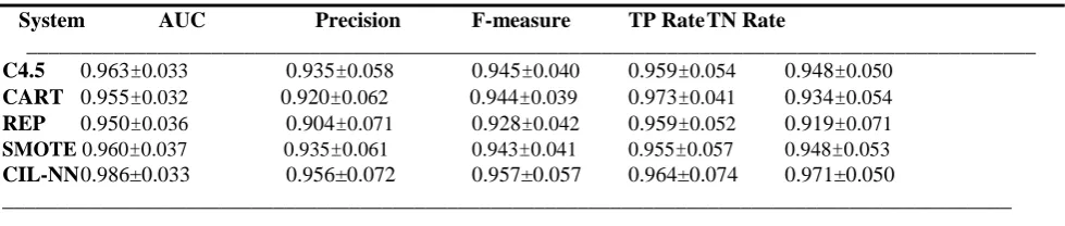
Table 2 Tenfold cross validation classification performance for Ecolicdataset

System AUC Precision F-measure TP Rate TN Rate

_____________________________________________________________________________________________

C4.5 0.963±0.033 0.935±0.058 0.945±0.040 0.959±0.054 0.948±0.050

CART 0.955±0.032 0.920±0.062 0.944±0.039 0.973±0.041 0.934±0.054

REP 0.950±0.036 0.904±0.071 0.928±0.042 0.959±0.052 0.919±0.071

SMOTE 0.960±0.037 0.935±0.061 0.943±0.041 0.955±0.057 0.948±0.053

CIL-NN 0.986±0.033 0.956±0.072 0.957±0.057 0.964±0.074 0.971±0.050

_____________________________________________________________________________________________

Table 3 Tenfold cross validation classification performance for Hepatitis dataset

System AUC Precision F-measure TP Rate TN Rate

C4.5 0.668±0.184 0.510±0.371 0.409±0.272 0.374±0.256 0.900±0.097

CART 0.563±0.126 0.232±0.334 0.179±0.235 0.169±0.236 0.928±0.094

REP 0.619±0.149 0.293±0.386 0.210±0.259 0.187±0.239 0.942±0.093

SMOTE 0.792±0.112 0.709±0.165 0.677±0.138 0.681±0.188 0.837±0.109

CIL-NN 0.820±0.175 0.807±0.197 0.754±0.170 0.758±0.242 0.778±0.230

Table 4 Tenfold cross validation performance for ionosphere dataset

_____________________________________________________________________________________________ System AUC Precision F-measure TP Rate TN Rate

_____________________________________________________________________________________________ C4.5 0.891±0.060 0.895±0.084 0.850±0.066 0.821±0.107 0.940±0.055

CART 0.896±0.059 0.868±0.096 0.841±0.070 0.803±0.112 0.921±0.066

REP 0.902±0.054 0.886±0.092 0.848±0.067 0.826±0.104 0.933±0.063

SMOTE 0.904±0.053 0.934±0.049 0.905±0.048 0.881±0.071 0.928±0.057

CIL-NN 0.948±0.048 0.945±0.061 0.892±0.070 0.852±0.110 0.940±0.071

_____________________________________________________________________________________________

Table 5 Tenfold cross validation performance for labor dataset

_____________________________________________________________________________________________ System AUC Precision F-measure TP Rate TN Rate

_____________________________________________________________________________________________ C4.5 0.726±0.224 0.696±0.359 0.636±0.312 0.640±0.349 0.833±0.127

CART 0.750±0.248 0.715±0.355 0.660±0.316 0.665±0.359 0.871±0.151

REP 0.767±0.232 0.698±0.346 0.650±0.299 0.665±0.334 0.765±0.194

SMOTE 0.833±0.127 0.871±0.151 0.793±0.132 0.765±0.194 0.847±0.187

CIL-NN 0.928±0.172 0.887±0.178 0.865±0.158 0.893±0.206 0.820±0.262

_________________________________________________________________________________________________

Table 6 Tenfold cross validation classification performance for breast_cancer dataset

_____________________________________________________________________________________________ System AUC Precision F-measure TP Rate TN Rate

____________________________________________________________________________________________ C4.5 0.606±0.087 0.753±0.042 0.838±0.040 0.947±0.060 0.260±0.141

CART 0.587±0.110 0.728±0.038 0.813±0.038 0.926±0.081 0.173±0.164

REP 0.578±0.116 0.721±0.037 0.805±0.042 0.917±0.087 0.151±0.164

SMOTE 0.717±0.084 0.710±0.075 0.730±0.076 0.763±0.117 0.622±0.137

Table 7 Tenfold cross validation classification performance for breast_w dataset

System AUC Precision F-measure TP Rate TN Rate

C4.5 0.957±0.034 0.965±0.026 0.962±0.021 0.959±0.033 0.932±0.052

CART 0.950±0.032 0.968±0.026 0.959±0.020 0.952±0.034 0.940±0.051

REP 0.957±0.030 0.965±0.030 0.960±0.021 0.957±0.033 0.931±0.060

SMOTE0.967±0.025 0.974±0.024 0.960±0.022 0.947±0.035 0.975±0.024

CIL-NN 0.990±0.013 0.973±0.033 0.963±0.027 0.954±0.043 0.974±0.032

Table 8 Tenfold cross validation classification performance for credit-g dataset

_____________________________________________________________________________________________ AUC Precision F-measure TP Rate TN Rate

_____________________________________________________________________________________________ C4.5 0.647±0.062 0.767±0.025 0.805±0.022 0.847±0.036 0.398±0.085

CART 0.716±0.055 0.779±0.030 0.820±0.028 0.869±0.047 0.421±0.102

REP 0.705±0.057 0.765±0.025 0.814±0.026 0.872±0.057 0.371±0.105

SMOTE 0.778±0.041 0.768±0.034 0.787±0.034 0.810±0.058 0.713±0.056

CIL-NN 0.722±0.062 0.704±0.063 0.696±0.063 0.695±0.100 0.652±0.108

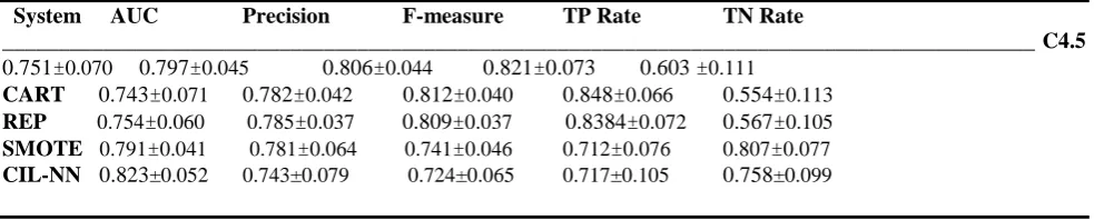
Table 9 Tenfold cross validation classification performance for Pima Diabetes dataset

System AUC Precision F-measure TP Rate TN Rate

_____________________________________________________________________________________________ C4.5

0.751±0.070 0.797±0.045 0.806±0.044 0.821±0.073 0.603 ±0.111

CART 0.743±0.071 0.782±0.042 0.812±0.040 0.848±0.066 0.554±0.113

REP 0.754±0.060 0.785±0.037 0.809±0.037 0.8384±0.072 0.567±0.105

SMOTE 0.791±0.041 0.781±0.064 0.741±0.046 0.712±0.076 0.807±0.077

CIL-NN 0.823±0.052 0.743±0.079 0.724±0.065 0.717±0.105 0.758±0.099

Table 10 Tenfold cross validation performance for vote dataset

____________________________________________________________________________________________ System AUC Precision F-measure TP Rate TN Rate

___________________________________________________________________________________________ C4.5 0.979±0.025 0.971±0.027 0.972±0.021 0.974±0.029 0.953±0.045

CART 0.973±0.027 0.971±0.028 0.966±0.022 0.961±0.037 0.953±0.046

REP 0.957±0.023 0.969±0.035 0.961±0.025 0.955±0.034 0.949±0.059

SMOTE 0.984±0.017 0.977±0.027 0.969±0.021 0.963±0.037 0.981±0.023

CIL-NN 0.991±0.015 0.965±0.047 0.943±0.042 0.926±0.064 0.972±0.040

______________________________________________________________________________________________________________

Table 11 Tenfold cross validation performance for Sonar dataset

_____________________________________________________________________________________________ System AUC Precision F-measure TP Rate TN Rate

_____________________________________________________________________________________________ C4.5 0.753±0.113 0.728±0.121 0.716±0.105 0.721±0.140 0.749±0.134

CART 0.721±0.106 0.709±0.118 0.672±0.106 0.652±0.137 0.756±0.121

REP 0.746±0.106 0.733±0.134 0.689±0.136 0.685±0.192 0.762±0.145

SMOTE 0.814±0.090 0.863±0.068 0.861±0.061 0.865±0.090 0.752±0.113

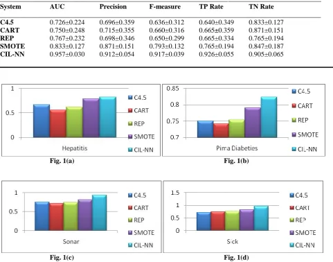
Table 12 Tenfold cross validation performance for Sick dataset

_____________________________________________________________________________________________ System AUC Precision F-measure TP Rate TN Rate

_____________________________________________________________________________________________ C4.5 0.726±0.224 0.696±0.359 0.636±0.312 0.640±0.349 0.833±0.127

CART 0.750±0.248 0.715±0.355 0.660±0.316 0.665±0.359 0.871±0.151

REP 0.767±0.232 0.698±0.346 0.650±0.299 0.665±0.334 0.765±0.194

SMOTE 0.833±0.127 0.871±0.151 0.793±0.132 0.765±0.194 0.847±0.187

CIL-NN 0.957±0.030 0.912±0.054 0.917±0.039 0.926±0.055 0.905±0.065

Fig. 1(a) Fig. 1(b)

Fig. 1(c) Fig. 1(d)

Fig. 1(a) – 1(d) Test results on AUC between the C4.5, CART, REP, SMOTE, and CIL-NN for Hepatitis, Pima Diabetes, Sonar and Sick datasets.

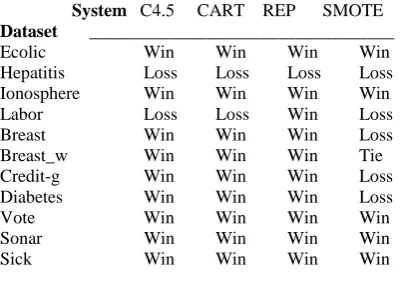
Table 13. Summary of results on AUC VsCIL-NN

_____________________________________________

System C4.5 CART REPSMOTE

Dataset __________________________________

Ecolic Win Win Win Win

Hepatitis Win Win Win Win Ionosphere Win Win Win Win Labor Win Win Win Win

Breast Win Win Win Loss

Breast_w Win Win Win Win

Credit-g Win Win Win Loss

Diabetes Win Win Win Win Vote Win Win Win Win Sonar Win Win Win Win Sick Win Win Win Win

____________________________________________

Table 14. Summary of results on Precision VsCIL-NN

_____________________________________________

System C4.5 CART REP SMOTE

Dataset __________________________________

Ecolic Win Win Win Win

Hepatitis Win Win Win Win Ionosphere Win Win Win Win Labor Win Win Win Win

Breast Loss Loss Loss Loss

Breast_w Win Win Win Tie

Credit-g Loss Loss Loss Loss Diabetes Loss Loss Loss Loss Vote Loss Loss Loss Loss Sonar Win Win Win Win Sick Win Win Win Win

Table 15. Summary of results on F-Measure VsCIL-NN

_____________________________________________

System C4.5 CART REP SMOTE

Dataset __________________________________

Ecolic Win Win Win Win

Hepatitis Win Win Win Win Ionosphere Win Win Win Loss Labor Win Win Win Win

Breast Loss Loss Loss Loss

Breast_w Tie Win Win Win

Credit-g Loss Loss Loss Loss Diabetes Loss Loss Loss Loss Vote Loss Loss Loss Loss Sonar Win Win Win Win Sick Win Win Win Win ____________________________________________________

Table 16.Summary of results on TP Rate Vs Prop.Algor. _____________________________________________

System C4.5 CART REP SMOTE Dataset __________________________________

Ecolic Loss Win Loss Loss

Hepatitis Win Win Win Win Ionosphere Win Win Win Loss Breast Loss Loss Loss Win Breast_w Loss Win Loss Win Credit-g Loss Loss Loss Loss Diabetes Loss Loss Loss Win Labor Win Win Win Win Vote Loss Loss Loss Loss Sonar Win Win Win Win Sick Win Win Win Win ____________________________________________

Table 17. Summary of results on TN Rate VsCIL-NN _____________________________________________

System C4.5 CART REP SMOTE Dataset __________________________________

Ecolic Win Win Win Win

Hepatitis Loss Loss Loss Loss Ionosphere Win Win Win Win Labor Loss Loss Win Loss

Breast Win Win Win Loss

Breast_w Win Win Win Tie

Credit-g Win Win Win Loss

Diabetes Win Win Win Loss Vote Win Win Win Win Sonar Win Win Win Win Sick Win Win Win Win ____________________________________________

In overall, from all the tables we can observe that the datasets Sick, Ecolic, Hepatitis, Ionosphere, Labor and Sonar have performed exceptionally well on all the measures against all the algorithms. One the Reason for the performance of proposed algorithm on all the above dataset is due to the very huge size of the dataset, irrelevant attributes present in the dataset, the multi class nature of the dataset and the majority and minority ratio of the datasets. The datasets Credit-g, Diabeties, Breast_w, Breast and Vote have not shown their performance up to their expectation. One the Reason for the underperformance of proposed algorithm is due to the problem in the minority set. Our proposed algorithm is not streamlining the instances present in the minority class. Another reason can be the verysmall size

of some dataset such as labor, and the final reason can be thenoises present in the dataset.

7. CONCLUSION

Class imbalance problem have given a scope for a new paradigm of algorithms in data mining. The traditional and benchmark algorithms are worthwhile for discovering hidden knowledge from the data sources, meanwhile Class imbalance Learning methods can improve the results which are very much critical in real world applications. In this paper we present the class imbalance problem paradigm, which exploits the subset filtering strategy in the supervised learning research area, and implement it with neural networks as its base learner. Experimental results show thatour proposed algorithm performed well in the case of multi class imbalance datasets. In our future work, we will apply our proposed algorithm to more learning tasks, especially high dimensional feature learning tasks.

8. REFERENCES

[1] J. Wu, S. C. Brubaker, M. D. Mullin, and J. M. Rehg, “Fast asymmetric learning for cascade face detection,” IEEE Trans. Pattern Anal. Mach. Intell., vol. 30, no. 3, pp. 369– 382, Mar. 2008.

[2] N. V. Chawla, N. Japkowicz, and A. Kotcz, Eds., Proc. ICML Workshop Learn. Imbalanced Data Sets, 2003.

[3] N. Japkowicz, Ed., Proc. AAAI Workshop Learn. Imbalanced Data Sets, 2000.\

[4] G. M.Weiss, “Mining with rarity: A unifying framework,” ACM SIGKDD Explor. Newslett., vol. 6, no. 1, pp. 7–19, Jun. 2004.

[5] N. V. Chawla, N. Japkowicz, and A. Kolcz, Eds., Special Issue Learning Imbalanced Datasets, SIGKDD Explor. Newsl.,vol. 6, no. 1, 2004.

[6] W.-Z. Lu and D.Wang, “Ground-level ozone prediction by support vector machine approach with a cost-sensitive classification scheme,” Sci. Total. Enviro., vol. 395, no. 2-3, pp. 109–116, 2008.

[7] Y.-M. Huang, C.-M. Hung, and H. C. Jiau, “Evaluation of neural networks and data mining methods on a credit assessment task for class imbalance problem,” Nonlinear Anal. R. World Appl., vol. 7, no. 4, pp. 720–747, 2006.

[8] D. Cieslak, N. Chawla, and A. Striegel, “Combating imbalance in network intrusion datasets,” in IEEE Int. Conf. Granular Comput., 2006, pp. 732–737.

[9] M. A. Mazurowski, P. A. Habas, J. M. Zurada, J. Y. Lo, J. A. Baker, and G. D. Tourassi, “Training neural network classifiers for medical decision making: The effects of imbalanced datasets on classification performance,” Neural Netw., vol. 21, no. 2–3, pp. 427–436, 2008.

[10]A.Freitas, A. Costa-Pereira, and P. Brazdil, “Cost-sensitive decision trees applied to medical data,” in Data Warehousing Knowl. Discov. (Lecture Notes Series in Computer Science), I. Song, J. Eder, and T. Nguyen, Eds.,

[11]K.Kilic¸,O¨ zgeUncu and I. B. Tu¨rksen, “Comparison of different strategies of utilizing fuzzy clustering in structure identification,” Inf. Sci., vol. 177, no. 23, pp. 5153–5162, 2007.

methodological approach to the classification of dermoscopy images,” Comput.Med. Imag. Grap., vol. 31, no. 6, pp. 362–373, 2007.

[13]X. Peng and I. King, “Robust BMPM training based on second-order cone programming and its application in medical diagnosis,” Neural Netw., vol. 21, no. 2–3, pp. 450–457, 2008.Berlin/Heidelberg, Germany: Springer, 2007, vol. 4654, pp. 303–312.

[14]RukshanBatuwita and Vasile Palade (2010) FSVM-CIL: Fuzzy Support Vector Machines for Class Imbalance Learning, IEEE TRANSACTIONS ON FUZZY SYSTEMS, VOL. 18, NO. 3, JUNE 2010, pp no:558-571.

[15]N. Japkowicz and S. Stephen, “The Class Imbalance Problem: A Systematic Study,” Intelligent Data Analysis, vol. 6, pp. 429-450, 2002.

[16]M. Kubat and S. Matwin, “Addressing the Curse of Imbalanced Training Sets: One-Sided Selection,” Proc. 14th Int’l Conf. Machine Learning, pp. 179-186, 1997.

[17]G.E.A.P.A. Batista, R.C. Prati, and M.C. Monard, “A Study of the Behavior of Several Methods for Balancing Machine Learning Training Data,” SIGKDD Explorations, vol. 6, pp. 20-29, 2004.1

[18]D. Cieslak and N. Chawla, “Learning decision trees for unbalanced data,” in Machine Learning and Knowledge Discovery in Databases. Berlin, Germany: Springer-Verlag, 2008, pp. 241–256.

[19]G.Weiss, “Mining with rarity: A unifying framework,” SIGKDD Explor.Newslett., vol. 6, no. 1, pp. 7–19, 2004.

[20]N. Chawla, K. Bowyer, and P. Kegelmeyer, “SMOTE: Synthetic minority over-sampling technique,” J. Artif. Intell. Res., vol. 16, pp. 321–357, 2002.

[21]J. Zhang and I. Mani, “KNN approach to unbalanced data distributions: A case study involving information extraction,” in Proc. Int. Conf. Mach. Learning, Workshop:

Learning Imbalanced Data Sets, Washington, DC, 2003, pp. 42–48.

[22]T. Jo and N. Japkowicz, “Class imbalances versus small disjuncts,” ACM SIGKDD Explor. Newslett., vol. 6, no. 1, pp. 40–49, 2004.

[23]S. Zou, Y. Huang, Y. Wang, J. Wang, and C. Zhou, “SVM learning from imbalanced data by GA sampling for protein domain prediction,” in Proc. 9th Int. Conf. Young Comput. Sci., Hunan, China, 2008, pp. 982– 987.

[24]A. Asuncion D. Newman. (2007). UCI Repository of Machine Learning Database (School of Information and Computer Science), Irvine, CA: Univ. of California

[Online]. Available:

http://www.ics.uci.edu/∼mlearn/MLRepository.htm

[25]J. R. Quinlan, C4.5: Programs for Machine Learning, 1st ed. San Mateo, CA: Morgan Kaufmann Publishers, 1993.

[26]C.-T. Su and Y.-H. Hsiao, “An evaluation of the robustness of MTS for imbalanced data,” IEEE Trans. Knowl. Data Eng., vol. 19, no. 10, pp. 1321– 1332, Oct. 2007.

[27][60] D. Drown, T. Khoshgoftaar, and N. Seliya, “Evolutionary sampling and software quality modeling of high-assurance systems,” IEEE Trans. Syst., Man, Cybern. A, Syst., Humans., vol. 39, no. 5, pp. 1097–1107, Sep. 2009.

[28]S. Garc´ıa, A. Fern´andez, and F. Herrera, “Enhancing the effectiveness and interpretability of decision tree and rule induction classifiers with evolutionary training set selection over imbalanced problems,” Appl. Soft Comput., vol. 9, no. 4, pp. 1304–1314, 2009.