Investigation of Performance Analysis of Classification Algorithm in Data Mining Dr. Mohd Ashraf 1, Dr. Zair Hussain *2

(1)

IJSRSET184425 | Received : 01 March | Accepted : 07 March 2018 | March-April-2018 [(4) 4 : 58-66]

58

Investigation of Performance Analysis of Classification

Algorithm in Data Mining

Dr. Mohd Ashraf1_{, Dr. Zair Hussain}*2

1_{Department of Computer Science & Engineering, Maulana Azad National Urdu University Hyderabad,}

Telangana, India

2_{Department of Information Technology, Maulana Azad National Urdu University Hyderabad, Telangana, India}

ABSTRACT

Data mining is now one of the most active field of research. Extracting those nuggets of information is becoming crucial and one of its important technique is classification. It helps to group the data in some predefined classes. Various techniques for classification exists which classifies the data using different algorithms. Each algorithm has its own area of best and worst performance. This paper concentrates on the four most famous algorithms, i.e., Decision Tree, Naïve Bayes, K Nearest Neighbour and Genetic Programming and the effect on their performance of time and accuracy when the number of instances are incrementally decreased. This paper will also investigate the difference in result when working with binary class or multiclass datasets and suggest the algorithms to follow when using certain kind of dataset.

Keywords : Decision Tree, Naïve Bayes, K-Nearest Neighbor, Genetic Programming, Accuracy

I. INTRODUCTION

In today‟s world, we are overwhelmed with data with is now increasing exponentially. The omnipresent computers makes it too easy to save things that previously we would have thrashed [2]. So, the information available is increasing, the understanding of that data is equally decreasing. The useful information is hidden in between all those layer of irrelevant data and we end up making decision based on our intuition rather than on informed logistics. With data mining we can extract the useful information from the vast amount of data and thus make an informed decision. The Wikipedia defines Data Mining as, “Data mining, an interdisciplinary subfield of computer science, is the computational process of discovering patterns in large data sets involving methods at the intersection of artificial intelligence, machine learning, statistics, and database systems. [3]”. Data mining tools perform data analysis

that helps to uncover data patterns and their relation that greatly contributes to knowledge base, business strategies, and medical and scientific research. The widening gap between data and information calls for a systematic development of data mining tools that will turn data tombs into “golden nuggets” of knowledge [8].

II. MACHINE LEARNING

Machine learning basically focuses on how the machines automatically learns in order to predict the result of an unseen data based on previous observation. Various machine learning algorithms are used for the classification in data mining.

Some of the machine learning strategies are: A. Supervised learning

(2)

with training examples. Typically these labels are class labels in classification problems. Supervised learning algorithms induce models from these training data and these models can be used to classify other unlabelled data [4]. It is basically classification.

For example, we can show a system with lots of images of animals with their names. The computer will save the attributes of those animals and when we show it some unseen data, it will recognize the animal using the training that was given to it.

B. Unsupervised Learning Strategy

In unsupervised learning, there is no target attribute or correct outputs. We just want to analyse the data to find some intrinsic structure in them. It‟s called Clustering.

For example, when talking about a supermarket, a person can buy an item A and B. another person comes and buys the same product as above. If this pattern continues then the learning strategy will realise that people who tends to buy A also tends to buy B and thus, it is beneficial for the supermarket owner to keep those two products near each other.

C. Reinforcement Learning Strategy

Another kind of machine learning is reinforcement learning. The training information provided to the learning system by the environment (external trainer) is in the form of a scalar reinforcement signal that constitutes a measure of how well the system operates. The learner is not told which actions to take, but rather must discover which actions yield the best reward, by trying each action in turn[1].

It is very similar to the behaviour psychology of learning better if we are given rewards. For example, an elevator can be given a reward every time it reaches to the correct floor.

D. Hybrid Learning Strategy

A hybrid strategy can be any strategy that combines two or more learning strategy. It is usually done in

order to harness the advantages of two or more strategy and to tackle their disadvantages.

By using the above strategies, the classification of the algorithms may vary. Different algorithms use different type of problems and every such algorithm have their own merits and demerits. Any classification algorithm can be evaluated using the following parameters:

1) Accuracy: It is defined as the percentage of correct predictions made by the total number of instances in a classification algorithm. Equation below states how accuracy can be calculated:

Accuracy= (no. of correct predictions)/

(no. of correct prediction + no. of incorrect prediction) ×100

2) Comprehensibility: It is the degree of simplicity and the understand ability in the rules generated after the classification. Higher degree of comprehensibility is required. More the number of nodes, less will be the comprehensibility. This is why we prefer a tree which has less number of nodes.

3) Training time: It is defined as the time that an algorithm takes to build a model on datasets. Minimum training time is desirable.

In essence, the goal in classification is to take an input vector x and to assign it to one of the K discrete classes Ck where k = 1,…, K.

III. CLASSIFICATION ALGORITHMS

The classification algorithms can further be divided into two categories:

A. Non-evolutionary classification algorithms

(3)

class label. Some common non-evolutionary classification algorithms are:

1. Decision Trees, 2. Naïve Bayes Classifiers

3. K-Nearest Neighbor Classifiers.

B. Evolutionary classification algorithms

Evolutionary algorithms (EAs) are search methods that take their inspiration from natural selection and survival of the fittest in the biological world. Several different techniques are grouped under the generic denomination of EA, which are

1. Genetic Algorithm (GA), 2. Genetic Programming (GP), 3. Evolutionary Strategies (ES) and 4. Evolutionary Programming (EP).

Some of the most famous algorithms are: 1. Decision Tree

A Decision Tree is a flow-chart-like tree structure. Here, each of the internal node represents a test on some attribute and each branch is the result of this test. Leaf nodes represent class distribution. The decision tree structure provides an explicit set of ―if-then rules rather than abstract mathematical equations, making the results easy to interpret [9].

A decision tree is a predictive model where and is one of the most common technique used for classification. It has many algorithms under it like J48, ID3, ADTree, LMT, NBTree etc. In decision tree we arrange all the attributes in form of a tree and then take the instances one by one and try to categorise them in the classes which is represented by the leaf nodes. Decision tree, thus, partition the whole input space into various cells where every cell belong to one class as defined in the class label. The partitioning is represented as a sequence of tests. Each interior node in the decision tree tests the value of some input variable, and the branches from the node are labelled with the possible results of the test [9]. The leaf nodes represent the cells and specify the class to return if that leaf node is reached. The classification of a specific input instance is thus performed by starting at the root node and,

depending on the results of the tests, following the appropriate branches until a leaf node is reached.

Advantages:

1. Comprehensibility is increased i.e. people can easily understand how the classification is done and the rules made for the classification.

2. Decision trees are inexpensive to construct

Problem:

1. When data is given incrementally, Decision Trees cannot be used directly.

2. When number of classes is more and data is large, the size of the decision tree becomes very large and thus decrease the comprehensibility.

2. Bayes Classifier

Bayesian classification is a kind of the statistical classification. It‟s an algorithm based on the probability. Bayesian algorithm‟s basic idea is using of the known prior probability and conditional probability parameter, based on Bayes theorem to calculate the corresponding posterior probability, and then obtained the posterior probability to infer and make decisions. Bayes classification models are based on the famous Bayes theorem. AODE, BayesNet, NaiveBayes are some of the algorithms under bayes classification.

(4)

have worked quite well in many complex real-world situations [9].

Advantage:

1. It requires short time for training the classifier. 2. Each training instance has an effect on

prediction and will increase or decrease the probability about the prediction.

Disadvantage:

1. The assumption of independence among

attributes is not true always and hence the accuracy of Naïve Bayes classifier is unstable [10].

3. k Nearest Neighbors Classifier

The k-nearest neighbor algorithm is amongst the simplest of all machine learning algorithms[1]: an object can be classified in respect to the votes from its neighbours. The class which gives majority of the votes win and the unlabelled object is classified in the winning class. „k‟ stands for considering k nearest neighbours. K is typically a positive and usually a small number. When k=1, the object is assigned to its single nearest neighbor. We can either assign equal weightage to all the neighbors or we can give more weightage to the neighbours which are nearer and less to the ones which are distant. Theses neighbours are usually a set of objects which are correctly classified and their class label is known. This classification using the neighbour can be thought of as the training part of the algorithm. There is no need for an explicit training of the algorithm. The k-nearest neighbor algorithm is sensitive to the local structure of the data.

Nearest neighbor classifiers are instance-based or lazy learners, in that they store all of the training samples and do not build a classifier until a new (unlabelled) sample needs to be classified. This contrasts with eager learning methods, such as decision tree, which construct a generalization model before receiving new samples to classify[9].

Advantage:

1. kNN classifiers require less training time 2. Are more accurate than decision tree.

Disadvantage:

1. They are sensitive to the choice of the similarity function selected for comparing instances. 2. As is assign equal weightage to all the instances,

the irrelevant data might create confusion during classification.

4. Genetic Programming

GP is an evolutionary algorithm-based methodology inspired by biological evolution of the survival of the fittest. It helps to find computer programs that perform a user-defined task in the best way possible. It is a specialization of GA where each individual is a computer program and uses a fitness measure to optimize this population.

GP steps to solve a problems[11]:

I. Generate an initial population (computer

programs) of random compositions of the functions and terminals of the problem.

II. Execute each program in the population and assign it a fitness value according to how well it solves the problem.

III. Create a new population of computer programs.

a) Copy the best existing programs

b) Create new computer programs by crossover c) Create new computer programs by mutation

The best computer program that appeared in any generation, the best-so-far solution, is designated as the result of genetic programming.

Advantages:

1. GP is a flexible evolutionary technique with some features that can be very appropriate for the evolution of classifiers. GP can be employed to construct classifiers using different kinds of

representations, e.g., decision trees,

(5)

2. The preferred criteria can be chosen like accuracy, timing etc. to express it as the fitness function.

3. GP can automatically eliminate irrelevant attributes unnecessary for the classification. 4. Its important tool for feature selection.

Disadvantage:

1. GP requires large training time. But once trained, the execution time of GP classifiers is much less. Hence, it can be used when there are no constraints regarding training time, but execution time matters..

IV. EXPERIMENT AND IMPLEMENTATION

The experiment is basically to assess the effect of decreasing the number of instances in a dataset on the accuracy and time of various classification algorithms. To implement this we used the tool Weka 3.6.11 developed by The University of Waikato, Hamilton, New Zealand [8]. Then we took the datasets from UCI library[6] and then used the algorithm „J48‟ of Decision Tree, „NaiveBayes‟ of Bayes and “IBk‟ of K Nearest Neighbour which are available in Weka Tool itself and used the Genetic Programming Algorithm by Yan Levasseur(Imagery, Vision and Artificial Intelligence Lab (LIVIA) Ecole de Technologie Superieure (ETS), Montreal, Canada) [7].

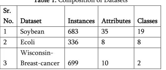
We wanted to test the effect of decrease in number of instances on multiclass as well as binary class data and so we took three types of Datasets with different kind of properties:

Table 1. Composition of Datasets Sr.

No. Dataset Instances Attributes Classes

1 Soybean 683 35 19

2 Ecoli 336 8 8

3

Wisconsin-Breast-cancer 699 10 2

As it can be seen, the number of classes varies widely. The next step was to incrementally decrease the

number of attributes and then running them through the various algorithms and noting down their performance.

We decremented the number of instance 10% each time and 5% in the end and the following data was obtained for the accuracy:

Table 2. Accuracy for Soybean Dataset[12] Dec.

%

No. of

instance DT NB k-NN GP

100 683 93.7 92.53 96.19 5.27

90 614 96.25 94.29 97.39 4.88

80 546 95.42 93.95 97.06 4.39

70 478 95.39 93.09 96.23 3.76

60 409 93.64 92.66 95.11 4.4

50 341 91.2 92.66 95.89 4.69

40 273 90.47 93.77 90.47 4.39

30 204 86.76 88.23 92.15 5.88

20 136 81.61 83.82 89.7 2.94

10 68 76.47 83.82 83.82 10.29

5 34 44.11 61.76 61.76 5.88

Table 3. Accuracy for Ecoli Dataset Dec.

%

No. of

instance DT NB

k-NN GP

100 336 84.22 85.41 80.35 81.25

90 302 87.74 84.76 93.04 88.41

80 268 87.31 84.7 93.28 85.82

70 235 85.53 86.8 91.48 87.23

60 201 88.55 88.05 89.05 83.58

50 168 89.28 86.3 85.71 87.5

40 134 88.05 86.56 81.34 82.08

30 100 87 84 81 84

20 67 88.05 83.58 83.58 85.07

10 33 78.78 84.84 82.81 90.9

(6)

Table 4. Accuracy For Breast Cancer Dataset Dec.

%

No. of

instance DT NB k-NN GP

100 699 94.56 95.99 94.99 94.7

90 629 96.5 96.02 97.77 96.34

80 559 94.99 96.24 98.03 95.88

70 489 95.5 96.32 97.54 95.5

60 419 95.22 95.94 97.37 95.94

50 349 95.98 95.98 95.98 96.56

40 279 96.05 96.05 96.77 96.41

30 209 97.6 96.65 97.6 97.6

20 139 97.12 97.84 95.68 97.84

10 69 92.75 95.65 95.65 97.1

5 32 85.29 94.11 97.05 94.12

The data obtained for the timing:

Table 5. Timing for Soybean Dataset

Dec. % No. of inst, DT time NB time k-NN time GP time

100 683 0.05 0 0.01 20.89

90 614 0.05 0 0 21.21

80 546 0.05 0 0.01 17.49

70 478 0.04 0 0 17.36

60 409 0.04 0.01 0 16.29

50 341 0.03 0 0 14.87

40 273 0.02 0 0 13.98

30 204 0.02 0 0 11.6

20 136 0.01 0 0 10

10 68 0.01 0 0 4.99

5 34 0 0 0 3.04

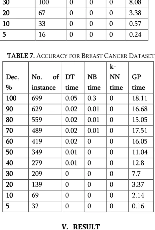
TABLE6.TIMING FOR ECOLI DATASET

Dec. %

No. of instance DT time NB time k-NN time GP time

100 336 0.02 0 0 16

90 302 0.02 0 0 13.71

80 268 0.02 0 0 14.4

70 235 0.01 0 0 12.28

60 201 0.01 0 0 12.64

50 168 0.01 0 0 12.7

40 134 0.01 0 0 9.16

30 100 0 0 0 8.08

20 67 0 0 0 3.38

10 33 0 0 0 0.57

5 16 0 0 0 0.24

TABLE7.ACCURACY FOR BREAST CANCER DATASET

Dec. %

No. of

instance DT time NB time k-NN time GP time

100 699 0.05 0.3 0 18.11

90 629 0.02 0.01 0 16.68

80 559 0.02 0.01 0 15.05

70 489 0.02 0.01 0 17.51

60 419 0.02 0 0 16.05

50 349 0.01 0 0 11.04

40 279 0.01 0 0 12.8

30 209 0 0 0 7.7

20 139 0 0 0 3.37

10 69 0 0 0 2.14

5 32 0 0 0 0.16

V. RESULT

After studying the above tables, it has been seen that the algorithms behave quite differently towards different type of datasets.

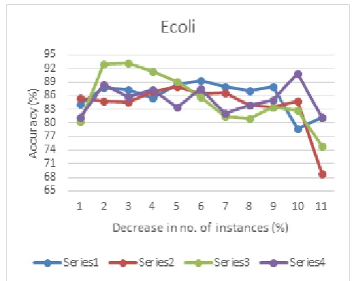
Consider the following graphs which are plotted using the information obtained.

Here, Series1 – Decision tree Series2 – NaiveBayes Series3 – Ibk

Series4 – Genetic Programming

(7)

decreased. Also the performance of GP was better and more consistent in the binary class dataset Breast Cancer as compared to the multiclass Dataset Ecoli.

Therefore, its desirable to use GP only when it‟s a binary class or have small number of classes and the number of instances are less. As it can be seen in both Ecoli and Breast cancer, the performance increased a little when only 90% of dataset was used as compared to 100%. In Ecoli, the performance kept on fluctuating. However, there was a consistency in the performance in Breast cancer as the number of instances was decreased except when the 5% data set was used.

Performance of GP when the timing was concern was really bad. It took the highest time among all the other algorithms. It is mostly due to the fact that its an evolutionary algorithm and thus generates rules first and then classifies the data.

Decision tree is not affected by the number of classes and its performance comparatively decreases first and then increases as the number of instances were decreased as in Soybean and Breast Cancer and it was rather unpredictable in Ecoli.

When the timing was concern, its performance was better than GP but worse than kNN and Bayes.

K-Nearest Neighbour was mostly consistent in its performance the whole time fluctuating only a bit on both the positive and negative side as compared to decision tree. Of all the other algorithms, this is the one which dosent seem to be much affected by the decreas in number of instance.

kNN performed best in the timing. It almost always took 0 seconds to perform the classification.

NaiveBayes followed a typical trend where it increased for a few reading and then started decreasing. It followed the same trend in all three cases and thus giving the best result in accuracy for

the reading with more amount of dataset and then start decreasing as the size of dataset decreases.

The timing for the bigger dataset was larger than kNN but smaller than decision tree. However, as the dataset start becoming smaller, the timing somewhat became comparable to that of kNN.

The performance of all the algorithms decreases dramatically at the end because only 5% dataset is remaining that that doesn‟t provide enough information in order to classify the dataset

Figure 1. Effect of decreasing the number of instance on the accuracy of the classification algorithms on the

Soybean Dataset

(8)

Soybean Dataset

VI. CONCLUSION

All the above four algorithms behave differently with the decrease in the number of instances. GP works poorly and erratically with multiclass data but increase its performance with decrease in number of instances in a binary class. However its time performance is really bad, so use this only when the timing is not a major concern. In decision tree, the performance first decreases and later on increased suggesting that decision tree is dependent on the size of datasets. So, it is advisable not to use it when the size of dataset is variable. kNN fluctuates mildly comparatively with the change in the number of instances suggesting that it doesn‟t depend on the dataset size much and can be used with a variable size dataset. NaiveBayes follows the trend where the accuracy increases in the start but then gradually decreases as the size of the dataset is decrease. This suggest that NaïveBayes does works better as the size of the dataset decreases, but after some threshold, the performance decreases. So, for working with NaïveBayes, its important to have an idea of an optimal dataset ideal for it. In the time performance, the kNN proves to be the best and its not dependent on the size of dataset. NaïveBayes dose depend on the size of dataset but works better than Decision Tree which also depends on the size of dataset

VII. FUTURE WORK

There are also many other algorithms that can be checked for the effect of decreasing the number of instances. Also, the effect of the same can also be checked within the various algorithms from the same class, e.g., we can check the above effect for the J48, ID3, C4.5 etc. Decision Tree algorithms.

VIII. REFERENCES

[1]. Radhika Kotecha, Vijay Ukani and Sanjay Garg, "An Empirical Analysis of Multiclass Classification Techniques in Data Mining",

INTERNATIONAL CONFERENCE ON

CURRENT TRENDS IN TECHNOLOGY, Vol.2, NUiCONE, DECEMBER, 2011

[2]. Ian H. Witten, Eibe Frank, Mark A. Hall, "What‟s It All About?," ] Data Mining Practical Machine Learning Tools and Techniques, Third Edition. USA, 2011.

[3]. Wikipedia. (2014, November, 11), Data

MiningOnline].Available:

http://en.wikipedia.org/wiki/Data_mining [4]. Matthieu Cord, and Sarah Jane Delany,

"Supervised Learning," P´adraig Cunningham. [5]. Harvinder Chauhan, Anu Chauhan, "Evaluating

Performance of Decision Tree Algorithms," International Journal of Scientific and Research Publications, Volume 4, Issue 4, April 2014 [6]. UCI repository. (2008, July, 15). Index of

/Datasets/UCI/arff Online]. Available:

http://repository.seasr.org/Datasets/UCI/arff/ [7]. leyan. (2013, April, 05). Genetic Programming

Classifier for Weka Online]. Available: http://sourceforge.net/projects/wekagp/

[8]. Machine Learning Group at the University of Waikato. (2014). Weka 3: Data Mining Software

in Java Online]. Availabe:

http://www.cs.waikato.ac.nz/ml/weka/

[9]. Jiawei Han and Micheline Kamber,

(9)

[10]. Medeswara Rao, Kondamudi, Sudhir Tirumalasetty, "Improved Clustering And Naïve Bayesian Based Binary Decision Tree With Bagging Approach," International Journal of Computer Trends and Technology (IJCTT) - volume 5 number 2 -Nov 2013

[11]. MIT Press. (2013). The GP Tutorial Online]. Available:

http://www.geneticprogramming.com/Tutorial/ [12]. R.S. Michalski and R.L. Chilausky "Learning by