REDUCTION OF LARGE SCALE
SYSTEMS BY EXTENDED BALANCED
TRUNCATION APPROCH
DEEPAK KUMAR
Department of Electrical Engineering, Institute of Technology, B.H.U., Varanasi, U.P. 221005, India
Dr. J. P. TIWARI
Department of Electrical Engineering, Institute of Technology, B.H.U., Varanasi, U.P. 221005, India
Dr. S. K. NAGAR
Department of Electrical Engineering, Institute of Technology, B.H.U., Varanasi, U.P. 221005, India
Abstract:
This paper deals with the development of an algorithmic approach for model order reduction based on balanced truncation technique. Reduction of stable systems based on balanced truncation is extended which may be applicable for any LTI (Linear time invariant) stable or unstable, minimal or non-minimal, continuous or discrete system. For reduction of unstable system, a system decomposition algorithm is given to decompose the unstable system into stable and unstable parts and then reduction of stable part is carried out and finally the subsystem addition of reduced stable part and already separated unstable part is done to get the final reduced model. The usefulness of the algorithm is shown by an illustrative example.
Keywords: Model order reduction; Balanced Truncation; Unstable systems; Real Schur transformation.
1. Introduction
Mathematical models of physical systems derived from theoretical considerations are usually complex and of high order. Such systems are difficult to be analyzed and also the designed controller becomes complex as well as costlier to implement. It is required to approximate these models by simpler models with reduced order which provides a good approximation of the original system.
Model reduction based on theory of balanced realization [1-6] was originally introduced by Moore [6]. In balanced realization theory, the term ‘balanced” is chosen for the system such that the input to state coupling and state to output coupling are weighted equally so that those state components which are weakly coupled to both the input and output are discarded. This theory is applicable for stable, minimal systems. It is based on forming a realization in which each state is equally controllable and equally observable from which reduced order model is obtained by truncating the least controllable and/or least observable states, and this model is called Balanced Truncated (BT) model. Pernebo and Silverman [7] presented the proof for several stages of works of Moore and reiterated that input/output behavior of the system does not change after truncation of least controllable and least observable states.
2. Algorithm for Balanced Realized Model Reduction for Stable systems
Considering standard linear time invariant (LTI) dynamical system
= + (1) = + (2)
where for each , ∈ ℂ, ∈ ℂ, ∈ ℂ are the vector of inputs, states and outputs, respectively. The matrices ∈ ℂ×, ∈ ℂ×, ∈ ℂ× and ∈ ℂ× are assumed to be constant. ℂ is n-dimensional complex euclidean space and ℂ× is space of complex × matrices. The transfer function of the system is:
= − + , for continuous time systems = − + , for discrete time systems
The notions of controllability and observability are central to the state space description of dynamical systems and if the eigenvalues of A are assumed to be strictly in the left half-plane, then we can define the controllability gramian for continuous time systems as
= ! "∞ #$ ∗"#$∗&'
( 3
and the observability gramian as
* = ! "#$∗
∗"#$&'
∞
( 4
By considering the corresponding matrix differential equations it is easily verified that P and Q satisfy the following linear matrix equations (Lyapunov equations)
+ ∗+ ∗= 0 (5)
∗* + * + ∗ = 0 (6)
Similarly for discrete time systems the controllability and observability gramians are
= - ./∞ . ∗∗.
./( 7
* = - ./∞ ∗.
./(
∗. 8
and P and Q satisfy the following linear matrix equations (Lyapunov equations)
∗− + ∗= 0 (9)
∗* − * + ∗ = 0 (10)
where, ‘*’ indicates the conjugate transpose of a matrix.
The steps of reduction algorithm are as below:
Step 1: Obtain Hankel Singular values (HSV) of the system by finding the square root of the eigenvalues of product of P and Q.
23 = 45. * (11) = 67, 78, 79,. . 7;, 7;<, . . . 7=
Assume that the magnitudes of HSV of the system is decreasingly ordered so that, 7≥ 78≥. . . ≥ 7?≥ ⋯ 7;> 0 and 7;<= ⋯ = 7= 0
where, n = order of the given original system k = the number of non-zero HSV ≈ minimal order of the system
r = the desired order of the reduced model.
Step 3: Perform singular value decomposition (SVD) of the controllability gramian P and observability gramian Q, and then proceed as algorithm developed by Safonov [8] for getting balanced truncated model of the order k which is the minimal order of the system. Singular value decomposition of P and Q can be obtained as
= CD3′ and * = CD3′ (12)
where Up, Vp, Uq and Vq are unitary matrices (orthogonal) and , *, D, C, 3, C, D and 3∈ E×
Step 4: Find similarity transformation matrices SL and SR such that
Let 3F= C4D, 3G = C4D and H = 3G′. 3
F (13)
Perform singular value decomposition of E such that
H = CIDI3I′, where, 3F, 3G, H, CI, DI and 3I∈ E×
To find similarity transformation matrices SL and SR [1, 2] for balanced realized model of the non-minimal system we truncate the elements of DI beyond k (the minimal order of the system or the number of non-zero HSV).
DJ?KL = DI1: O, 1: O, where DJ?KL ∈ E;×; (14)
Finally the transformation matrices are obtained as,
G= 3G. CI. DJ?KL /8 (15)
F = 3F. CI. DJ?KL/8 where G and F∈ E×; (16)
Step 5: The balanced realized model of order k, for the kth order minimal system is (for original nth order system in case of non-minimal systems) is:
QRS= TQRS | QRS
QRS | QRSV = W
G′F | G′
F | X 17
Step 6. The above balanced realized minimal model is the combination of strong and weak subsystems as below:
→
←
→
←
−
−
=
r k r
r k r
D C
C
B B
A A
A A
Gbal
2 1
2 1 22
21
12 11
= T
Y
V + T888 Y 8
0 V 18 = Z[\ ]"^ + _"`O ]"^
[ ]" Z"`a"& [ ]" "ba^a`"&
The balanced truncated model ?_QJof desired order r is obtained by truncating the terms from kthorder balanced model QRS, as below:
→ ←
=
r
r
d c
b a
bt r
G
1
1 11
_
= Z[\ ]"^ Z′ℎ [Z&"Z e f[&"b
3. Extension of Balanced Realized Model reduction technique to Unstable systems
In this section model reduction using balanced truncation is extended for unstable systems. Since the Lyapunov equations only exist for stable systems, therefore the algorithm developed for the stable system is directly not applicable to unstable systems, but BT algorithm can be used for reduction of unstable systems after decomposition of original systems as below:
3.1. Unstable System Decomposition
The decomposition technique developed here contains two stages of transformations. In first stage the block form of real Schur transformation facilitated in Robust Control Toolbox of MATLAB [11] has been used. In second stage of transformation, the generalized Lyapunov equation [9] is solved and completely decoupled stable and unstable systems are obtained.
The decomposition algorithm consists of following steps:
Step 1: Let the system represented by equation (1) be an unstable system. Transform this system using an unitary matrix U in block diagonal upper Schur form [11], such that the eigenvalues of the transformed system are arranged in increasing order of its real components (in case of continuous time systems) and arranged in increasing order of its absolute value of its eigenvalues (in case of discrete time systems). If x denotes the original system states then the first stage transformation matrix U (the unitary matrix) and the transformed system states xt may be related as = CJ. Thus, the first stage transformed system becomes,
= = D t C t B t A D CU B U AU U t G ' ' (19) → ← → ← − − = m n m m n m D t C t C t B t B t At A t A 2 1 2 1 22
011 12
where n denotes order of the system, m denotes the number of stable eigenvalues and n-m denotes the number of unstable eigenvalues.
Step 2: The transformed system of step (1), contains a coupling term At12. To bring transformed system into completely decoupled form, we solve the general form of Lyapunov equation
J − J88+ J8= 0 (20)
Obtain the value of S and proceed for second stage of transformation using xt=WX, where X is the final stage
transformed state and W is the final stage transformation matrix. The second stage transformation matrix W is given as
h = i
j .
⋯ . ⋯
0 . j
k (21)
where Im and In-m are identity matrix of size and n-m, respectively.
The important property of W is that W-1 can be obtained simply by replacing S with –S. i.e.
h = i⋯ .j . −⋯
0 . j
k (22)
Thus, W-1 always exists and hence never found ill-conditioned. Using W, we obtain the completely decoupled system (Gd) as,
l = Wh
Jh | h J
JC | X
→ ← → ← − − = m n m m n m D C C B B A A 2 1 2 1 22 0 0 11
where J= C′C,
J= C′ and J= C are obtained from step (1).
This transformed model may be decomposed into stable and unstable as
l= T
Y
V + T888 Y 8
3.2. Balanced Realized Reduced model for decomposed stable system
Separated stable subsystem GS = {As, Bs, Cs, Ds} as obtained in equation (23) containing m stable eigenvalues, be described in state space as
o= T YV
To determine rth order balanced truncated reduced model, we need to determine the full order balanced model of stable subsystem, Gs. The full order balanced realized model of the system represented by equation (1),(2) will be the combination of strong and weak subsystem which is given by
= bal D bal C bal B bal A bal s G _ → ← → ← − − = r m r r m r d c c b b a a a a 2 1 2 1 22 21 12 11
So, the rth order balanced truncated reduced model can be obtained from equation (18) which is given by
o?_QJ= T`p
Y
]
& V
3.3. Overall Reduced order model for original unstable system
The balanced truncated reduced model of unstable system is obtained by obtaining the balanced truncated model of the decomposed stable part and directly adding it to intact decomposed unstable part, obtained in equation (23) as below:
?_QJ= o?_QJ+ K (24)
Here, it is important to note that the balanced truncated reduced model of unstable system (Gr_bt) is however not balanced but its name is based on the fact that it has been derived from balancing and truncating the stable part of Gs (i.e., derived from the balanced truncated model, Gs_bal).
4. Illustrative Example
The data of 7th order, 2 input and 2 output synchronous machine connected to an infinite busbar through a transmission line considered by Lastman and Sinha [10] is given as below:
− − − − − − − − − − − − − = 0 0 0 0 0 0 0 1 0 0 0 0 0 0 0 0 0 1 0 0 05 . 118 25 . 107 0 0 0 0 0 0 0 0 998 . 57 83 . 162 4 . 377 449 . 89 57 . 157 579 . 68 0 0 0 0 555 . 43 846 . 16 079 . 25 0 0 0 353 . 89 32 . 251 58 . 376 8726 . 9 2036 . 6 054 . 15 827 . 66 24 . 162 0 99 . 376 0 0 4363 . 1 53002 . 0 0176 . 2 0 0 0 0 0 0 0 0 0 0 99 . 376 21133 . 0 0 49947 . 0 64719 . 0 26303 . 0 36992 . 0 1445 . 0 0 2113 . 0 G
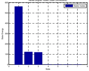
The hankel singular values are
23 = 6561.8055, 121.7607, 117.8798, 0.0947, 0.001 0.00=
Bar chart of Hankel singular values is plotted in Fig. 1 to determine which states are weakly coupled to the system and can be discarded.
Fig. 1 Bar-chart of the HSVs of the 7th
order power system model
0 1 2 3 4 5 6 7 8
0 100 200 300 400 500 600
Hankel Singular Values (State Contributions)
The magnitude of hankel singular values and bar-chart show that that only first three HSV are significant. So, the 3rd order model will be appropriate. From the algorithm given in section II and III the balanced truncated 3rd order reduced model is
?_QJ=
t u u u u
v−0.1988 −0.5062 0.054170.5062 −0.9124 9.352 0.05281 −9.35 −0.02611
0.01299 0.002405 0.3717 14.94 14.91 −2.453 w
w
−14.94 0.05122 14.91 0.04161 2.414 0.572
0 00 0 x y y y y z
3rd order reduced model obtained by Lastman and Sinha [10] using dominant eigenvalue retention method is:
?_(=
t u u u u
v−0.6085 −0.2312 −0.1472376.99 0 0 2.9463 −0.5037 −0.5261
1 0 0
0 1 0 w
w
0.8844 0.2134
0 0
363.2587 −0.0168 0 00 0
x y y y y z
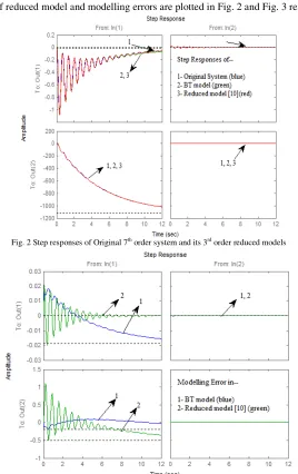
The step responses of reduced model and modelling errors are plotted in Fig. 2 and Fig. 3 respectively.
Fig. 2 Step responses of Original 7th
order system and its 3rd
order reduced models
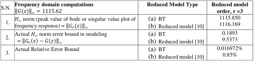
The nature of step responses of proposed model and modelling errors show the advantage and usefulness of the balanced truncated model over the model obtained by Lastman and Sinha [10] using dominant eigenvalue retention method. The balanced truncated model possesses maximum error in low frequency region. Therefore, such models are more appropriate for high frequency applications. The frequency domain calculations for original and reduced models are summarized in Table 1.
Table 1. Frequency Domain Computations for Models
S.N. Frequency domain computations ‖‖∞= 1115.62 Reduced Model Type Reduced model
order, r =3
1. 2∞ norm (peak value of bode or singular value plot of frequency response) = ‖?‖∞
(a)
BT(b)
Reduced model [10]1115.850 1116.169
2. Actual 2∞ norm error bound in modeling = ‖? − ‖∞
(a)
BT(b)
Reduced model [10]0.1893 9.5373
3. Actual Relative Error Bound
(a)
BT(b)
Reduced model [10]0.016972% 0.85%
Conclusion
This paper highlights the extension of balanced realization theory for obtaining reduced order model for stable/unstable, minimal/non-minimal, continuous/discrete LTI systems. As balanced realization theory is applicable for only stable, minimal systems. Extension of balanced truncation technique has been proposed which is applicable for reduction of any stable/unstable systems. For the reduction of unstable system a system decomposition technique based on real Schur algorithm is given which decompose system into stable and unstable subsystems. Final reduced model is obtained by adding reduced stable part and already separated unstable part. Frequency domain priori 2∞ norm error bound is calculated and step responses of original system, reduced models and modelling error transfer functions are compared.
References
[1] Singh, S. K.; Nagar, S. K.; Pal, J. (2006): Balanced Realized Reduced modelof a non-minimal system with DC gain preservation, IEEE conference on Industrial technology, ICIC 2006, IIT Bombay, pp. 1522-1527.
[2] Singh, S. K.; Nagar, S. K. (2004): BSPA based 28/2∞ controller reduction”, IEEE India annual conference 2004, INDICON 2004, Indian Institute of Technology, Kharagpur, pp. 195-198.
[3] Singh, S. K.; Nagar, S. K. (2004) “An algorithmic approach for system decomposition and balanced realized model reduction” Journal of the Franklin Institute 341, Elsevier, pp. 615–630.
[4] Kumar, Deepak; Tewari, J. P.; Nagar, S. K. (2011) : Model reduction of SISO systems by an improved technique based on Balanced approach, National conference on Instrumentationa and control, Kolkata.
[5] Glover, K. (1984): All optimal hankel norm approximation of linear multivariable systems and their |∞ error bounds , Int. J. Contr. 39, 1115–1193.
[6] Moore, B. C. (1981): Principal component analysis in linear systems: controllability, observability and model reduction , IEEE Trans. Automat. Contr. 26,17–32.
[7] Pernebo, L.; Silverman, L. M. (1982): Model reduction via balanced state space representations, IEEE Trans Automat. Contr. 27 (2), 382–387.
[8] Safonov, M.G.; Chiang G. (1989): A Schur method for balanced truncation model reduction, IEEE Transaction of Automatic Contr. 34 (7), 729-733
[9] Mahmoud, M.S.; Singh, M.G. (1981): Large Scale System Modelling, Pergamon Press, Oxford.
[10] Lastman, G. J.; Sinha, N. K.; Rozsa, P. (1984): On the selection of the states to be retained in the reduced order model, IEE proceedings, vol. 131, pp. 15-22.