An investigation of diffuser for water current turbine application using CFD

An investigation of diffuser for water

current turbine application using CFD

Palapum khunthongjan

Ph.D. Candiate in Mechanical Engineering, Faculty of Engineering, Ubon Ratchathani University,Thailand.

Adun janyalertadun

Assistance Professor in Mechanical Engineering, Faculty of Engineering, Ubon Ratchathani University,Thailand.

Abstract

The use of water stream as the energy resource has long time happenedbut its velocity is pretty low so it’s not found in wide range of uses. Here the study purposes accelerate water velocity by installing diffuser. The problems were analyzed by one dimension analysis and computational fluid dynamics (CFD); domain of flowing problem will cover diffuser and turbine area that be substituted by porous jump condition. In this study flow identified as axisymmetric steady flow, inlet boundary identified as uniform flow, sizes of diffuser was still but the diffuser angle. The study found that the more widen diffuser angle, the more velocity of water stream toward the turbine. A 20° angle of diffuser was to add 1.9 times of water velocity and 1.7 times of energy if compared to the diffuser-uninstalled turbine. If the angle was about 0-20°and 50-70° the force toward diffuser became high instantly; where as the force toward the rotor will be still and the maximum rate of rotor power augmentation possibly was 3.5.

Key word: Water current turbine, Diffuser, Computational fluid dynamics, Power augmentation factor

Symbol:

a

_{= axial induction factor}



_{= Diffuser area ration}



_{= Back pressure velocity ration}

C

pi _{= pressure coefficient at location i}

diff T

C

_,

= Trust coefficient of diffuser

C

T,total = Total trust coefficient of diffuser plus rotor

rotor T

C

_,

= Trust coefficient of rotor V0 = free stream velocity

V1 = velocity at nozzle of diffuser V1 = velocity at nozzle of diffuser

V2 = velocity at back of rotor V3 = velocity at exit of diffuser

1. Introduction

The uses of kinetic energy of water stream for generating electricity or pumping has been studied for times which mainly aim to use in remote area like the study of Peter Fraenkel ‘Vertical axis Darrieus toror’ in 1976-1984 (referred from 1) and any others (3-9). According to the kinetic energy use from water stream, a wind turbine-based knowledge at commercial level can appropriately be applied to that its capacity of energy distribution is as BETZ rules. The Axial flow turbine has its maximum power coefficient (CP ) 16/27. Though its

capacity was later 45% developed, still it challenges the researcher to continue strengthen its effectiveness. Another way to do so is to set up the diffuser that can be both wind turbine and water turbine as found in the wind turbine study by D.G. Phillips et al. (10, 11) from the University of Auckland, New Zealand and Toshiio Matsushima et al., (12) Yuji Ohya et al., (13) and etc. But in the study of Gerald J.W. van Bussel (14) indicates that no any power augmentation factor was more than 3. Referring to the theory the power coefficient probably was 2.5 but the price of diffuser is somewhat high.

In addition, several countries – Canada, Ireland, England, USA (18-22), Australia, and Portuguese – have been developing water turbine for electricity which are all on process, examining the model mechanic, and for commerce.

Through the capacity of water stream as the energy resource and the occurrence of the apply of water turbine at low flow velocity, this article means to study functions and performance of diffuser as to be the output power accelerator of horizontal axis water current turbine in order to be applied in the Northeast of Thailand that has two main rivers - Munr and Chii. The velocity of water current is between 0-1.3m/s which formed in two dimension system by computational fluid dynamic (CFD). The sttractive factors are effect of diffuser angle, maximum augmentation factor, and rotor power coefficient due to use to design diffuser for wind turbine later.

2. Materials and Methods

2.1 One dimension analysis (referred from 14)

In case of Empty diffuser

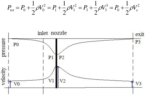
From figure 1 the surface of diffuser outlet will be referring point, front and back space of diffuser equal atmospheric pressure(

P

0_{). The continuity equation by Bernoulli shows that total pressure equals:}

2 0

3 3 3 2 1 1 2 0 0

2

1

2

1

2

1

2

1

e

tot

P

V

P

V

P

V

P

V

P

























Figure 1. Relationship between pressure and velocity within the diffuser

From the continuity equation shows the coherence between the inlet velocity (

V

1_{), outlet velocity (}

V

3

) and diffuser area ratio(



)

V

1





V

3

and

V

3





V

0



_{= Back pressure velocity ratio,}

0

V

= free stream velocity in front of diffuser



_{use of Back pressure velocity ratio,}

0

V

use of free stream velocity in front of diffuser In terms of installed the turbine:

0

3

(

1

a

)

V

V







0

1

(

1

a

)

V

a

_{= Axial induction factor}

Rotor power coefficient

C

P,rotor

2

,

4

a

(

1

a

)

C

_Protor







Power coefficient at diffuser exit

C

P,exit

2

,

4

a

(

1

a

)

C

_Pexit







Total trust coefficient

C

T,total

C

T,total





4

a

(

1



a

)

Trust coefficient of diffuser

C

T,diff

C

T,diff



C

T,total



C

T,rotor



(





1

)

4

a

(

1



a

)

2.2 Computational fluid dynamics (CFD)

Computational fluid dynamics Computational Fluid Dynamics (CFD) is a branch of fluid mechanics that uses numerical methods and algorithms to solve and analyze problems that involve fluid flows. Computers are used to perform the calculations required to simulate the interaction of liquids and gases with surfaces defined by boundary conditions. There are three main processes – pre-processor, calculation processing and post-processor. Here the fluent 6.3 commercial code 2 dimensions with the finite volume method.

Governing equation

Described equation of flow is continuity and Reynolds-averages Naviaers – Stokes equations:

0







i i

U

x

(1) i j i j i j I j i i i

j

u

u

F

x

U

x

U

v

x

x

P

U

x

U



































































1

(2)

When

u

i

u

j is Reynolds Stresses and



,

P

,

U

i

,

u

i_and

v

_{are density, mean static pressure, mean} velocity, turbulent fluctuation, and kinematic viscosity respectively and

F

i _{is body-force term that means load in} the system.

To calculate the Reynolds Stresses depends on Reynolds analogy; eddy viscosity model that is presented as turbulent viscosity hypothesis.

Turbulent viscosity hypothesis

Reynolds Stresses is separated to isotropic part;

u

i

u

j



ij (vertical factor with equal attribute to all

directions and anisotropic part). So, anisotropic part

a



u

i

u

j



u

i

u

j



ij _and

k



 

1

/

2

u

i

u

j_{. From the} turbulent viscosity hypothesis the anisotropic part will vary directly with mean rate of strain as following equation;

ij j

i

u

k

u

a



2

1



























i j j i t ij j i

x

u

x

u

k

u

u













2

1

t



RNG k–ε, turbulence model,















2







_t

f

k

Computational conditions

Figure 2. Domain of the problem

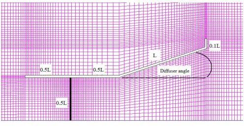
Domain of flow problem will cover diffuser, turbine area that specified as wall and porous jump condition. The inlet boundary set as the uniform flow velocity, outlet boundary is as outflow, Top wall is as moving wall, and bottom wall is as axisymmetric shown in figure 2 and 3. Domain will be drawn in Gambit Program before be computerized by Fluent 6.3. Problem domain will be separated by quadrilateral grids into approximately 11,000 cells. Anyway, grids will be dense around diffuser wall and turbine area.

Figure 3. Diffuser dimension and Grid system

The study set the flow as axisymmetric steady flow It is segregated solver, whereas turbulence model is RNG

k





model. The standard near wall function was chosen for near wall treatment method with 10-6 of the convergence criterion. Sizes of diffuser are unchanged but diffuser angle as in figure 3 that changed from 0-90°. The porous medium will be from Darcy's Law and an additional inertial loss term as the equation.













_





2

2

2

1

v

C

v

p









_{is the laminar fluid viscosity,}



_{is the permeability of the medium,}

C

2_{is the pressure-jump coefficient,}



is the velocity normal to the porous face, and



m

is the thickness of the medium.

3. Results and Discussion Simulation and results

Y Plus check

0 50 100 150 200 250 300

0 0.05 0.1 0.15 0.2 0.25

Position

W

al

l Y

Pl

us

Figure 4. Yplus of Diffuser wall

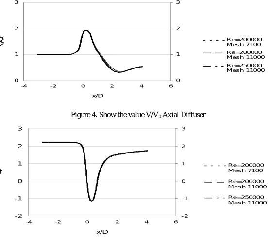
The evaluation of grid and Reynolds numbers per domain is split into 11,000 and 7,100 quadrilateral cells and calculate Reynolds number at 200,000 and 250,000 respectively. Its result – increased velocity (V/V0)

and pressure coefficient (Cp) are slightly different as figure 5 and figure 6 that will be cited later.

0 1 2 3

-4 -2 0 2 4 6

x/D

V

/V

0

0 1 2 3

Re=200000 Mesh 7100 Re=200000 Mesh 11000 Re=250000 Mesh 11000

Figure 4. Show the value V/V0 Axial Diffuser

-2 -1 0 1 2 3

-4 -2 0 2 4 6

x/D

C

p

-2 -1 0 1 2 3

Re=200000 Mesh 7100 Re=200000 Mesh 11000 Re=250000 Mesh 11000

Flow Inside the Diffuser

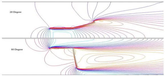
Figure 6. Result of Simulation 2D show velocity contour at Diffuser angle = 20 and 80 degree.

Figure 6: the result of Simulation 2D tells velocity contour when

C

T,rotor =0 compared to the angle of diffuser at 20° and 80°. To increase angle of diffuser lengthens the velocity contour; whereas radial velocity becomes more different and happens more splits at the flow duct.

Figure 7:

C

T,rotor=0; shows the velocity of axial flow (X), 0 = Diffuser inlet 1 (Diffuser exit). The velocity of axial flow of diffuser will be faster where the diffuser angle is increased.

0 0.5 1 1.5 2 2.5 3 3.5 4

-6 -5 -4 -3 -2 -1 0 1 2 3 4 5 6 7 8 9

x/D

V1

/V

0

deg90 deg70 deg60 deg40 deg20 deg00

Figure 7. Show V1/V0 Axial Diffuser

Besides, at the front inlet boundary the velocity will be increasing from -2 when the angle equals 90° and from -0.5 when the angle equals 20 approximately. The main function of diffuser can be explained that through the theory of continuity when the surface of diffuser around the outlet boundary is widen out, the less pressure and velocity to the exit of diffuser’s inner flow are. The fluid will try to maintain its flow condition; so it accelerates the velocity at the inlet boundary of diffuser and happen to maximum speed around the inlet boundary of diffuser.

Diffuser augmentation,



0.0 0.5 1.0 1.5 2.0 2.5 3.0 3.5 4.0

0 10 20 30 40 50 60 70 80 90

Diffuser angle, Degree

B

e

ta

,G

a

m

m

a

, D

im

e

n

s

io

n

le

s

Figure 8a. Diffuser area ratio

(



)

Back pressure velocity ratio

(



)

, Diffuser augmentation

(



)

, VS. Diffuser angle

0 0.5 1 1.5 2 2.5 3 3.5 4

0 20 40 60 80

Diffuser angle, Degree

B

a

ck p

re

ss

u

re

v

e

lo

ci

ty

r

a

ti

o

-6 -5 -4 -3 -2 -1 0

E

x

it

pr

es

s

ur

ec

oef

fi

c

ient

,C

p

3

Back pressure velocity ratio,γ Exit pressure coefficient,Cp3

Figure 8b. Back pressure velocity ratio

(



)

, Exit pressure coefficient

C

P,Exit VS. Diffuser angle

Figure 8a: shows diffuser area ratio,

(



)

Back pressure velocity ratio,

(



)

, Diffuser augmentation

(



)

, VS Diffuser angle.



values more than 1 when the angle is more 0° and get increasing if the angle of diffuser is widen out. It means that there’s negative back pressure at the exit of the diffuser as seen in figure 8b. From figure 8a probably the angle of diffuser is separated into 4 phases that are 0-20, 20-50, 50-70, and 70-90. Phase 0-20 both



and



value more. Phase 2 20-50



° looks decreased but



values increasingly. Phase 3 50-70



° is constant but



and



are raised. Last phase 70-90°



,



and



are all unchanged. When the angle is wider than 20°, the maximum velocity at the axial flow of diffuser is getting faster, and radial diffuseness of velocity is sparse those give the ratio of

V

1

/

V

3 ₍



_{) lower and higher}



)

/

(

V

₃

V

₀

value. But the multiplication of



and



is up. Therefore, it can be defined as



significantly effects on diffuser augmentation

(



)

while



will be important if its angle is less than 20°

Trust loading coefficient

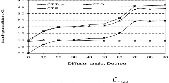
Figure 9: to widen angle of diffuser causes diffuser augmentation be higher; while trust forced toward diffuser is obviously getting up between the phase of 0-20° and 50-70° but slightly influence on trust coefficient of rotor. It can be defined as if we build diffuser with the more degree in order to keep energy as much as we require, durable structure is needed for the increasing trust.

0.0 0.5 1.0 1.5 2.0 2.5 3.0 3.5 4.0

0 10 20 30 40 50 60 70 80 90

Diffuser angle, Degree

Lo

adi

ng c

oeef

fi

c

ien

t

,C

t

CT Total CT D CT R

Figure 9. Disk loading coefficient,

C

T,total,

diff T

C

_,

Effect of trust coefficient of rotor

0 0.2 0.4 0.6 0.8 1 1.2 1.4

0 0.2 0.4 0.6 0.8 1

Trust coefficient of rotor , Ct rotor

Ro

to

r p

ow

er

c

oef

fic

ient

,

C

p

1.0 m/s 2.0 m/s

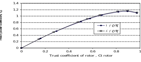
Figure 10. Trust coefficient of rotor vs Power coefficient Cp

Figure 10: This shows result of simulation when initial degree of diffuser equals 20°. When trust coefficient of diffuser gets higher, the more the power coefficient is and power coefficient will reach the maximum rate when trust coefficient of diffuser is about 0.9. Through graph above it’s noticeable that when the velocity is changed from 1 to 2 m/s rotor power coefficient will slightly be up.

Rotor power augmentation

0.0 1.0 2.0 3.0 4.0 5.0

0 10 20 30 40 50 60 70 80 90

Diffuser angle, Degree

0.0 0.2 0.4 0.6 0.8 1.0 1.2 1.4

A

x

ia

l i

ndu

c

ti

on

fac

tor

,

a

V1/V0 Rotor power augmentation ϐƔ

Axial induction factor

Figure 11. Show V1/V0, Rotor power augmentation, Diffuser augmentation,



axial induction factor, a VS Diffuser angle, degree

Figure 11: It shows the ratio of changed augmentation (V1/V0), Rotor power augmentation (Rotor

power coefficient divided by Power coefficient of bare turbine), diffuser augmentation,



and axial induction factor. In the calculation a is the coefficient = 1/3. We will see that the changed augmentation at turbine area V1/V0), Rotor power augmentation and diffuser augmentation,



is a bit different because the maximum rate

of rotor power augmentation after calculating is 3.5.

4. Concluding remark

Widening degree of diffuser causes more augmentation of V1/V0 which will be rapidly growing during

the phase 0-20° and 50-70°. If the degree approximately equals 20°-50°, the augmentation will not change much; while the angle is about 70°-90° V1/V0 will be fixed. Trust toward rotor will be steady if the

augmentation is increased; where as trust toward diffuser will be higher similarly. So, before contouring it’s necessary to evaluate trust. The effective factors towards V1/V0 include Diffuser area ratio,

(



)

and Back

pressure velocity ratio

(



)

that the latter one indicates it’s increasing according to degree of diffuser which is good to performance of diffuser angle. At the same time



will be lower if the angle degree is more than 20° and will 1 as approximation when the degree is up to 50°. Via the study the rotor power augmentation will reach the maximum rate at 3.5 when the angle degree equals 90° and when the angle degree is about 20°- 50° the rotor power augmentation will be about 2.

Later soon there will be the examination of diffuser in order to find the difference between simulation and its real performance.

5. Acknowledgement

Thanks to the Electricity Generating Authority of Thailand to fund the research. 6. References

[1] FINAL REPORT ON PRELIMINARY WORKS ASSOCIATED WITH 1MW TIDAL TURBINE PROJECT REFERENCE: T/06/00233/00/00 URN 06/2046 Contractors Sea Generation Ltd Prepared by David Ainsworth, Jeremy Thake Marine Current Turbines Ltd

[2] Peter Fraenkel, 2006 Tidal current energy technologies, Marine current turbine limited, the green, stoke giffford, Bristol BS 34 8PD ,UK Ibis(2006),148 145-151

[3] F.L Ponta and P.M.Jacovki, Marine current power generation by diffuser- augmented floating hydro turbines, Renewable energy 33(2008), 665-673

[4] Fernando Ponta and Gautam Shankar Dutt ,An improved vertical-axis water-current turbine incorporating a channeling device, Renewable energy 20(2000), 223-241

[5] Lukes Myyers, A.S.Bahaj ,Power out put performance characteristics of horizontal axis marine current turbine, Renewable energy 31(2006), 197-208

[6] A.S.Bahaj, L.E. Myers Fundamentals applicable to the utilization of marine current turbine for energy production, Renewable energy 28(2003), 2205-2211

[7] M.J.Khan, M.T. Iqbal and J.E.Quaicoe, River current energy conversion system: Progress , prospects and challenges, Reneable and sustainable energy reviews 12(2008)2177-2193

[8] 8.S.Kiho,M.Shiono and K.Suzuki, The power generation from tidal currents by Darrieus turbine, Department of Electric Engineering , College of Science & Technology, Nihon University Tokyo, Japan

[9] G MacPherson-Grant ,The Advantages of Ducted over Unducted Turbines Rotech engineering Ltd.6th European Wave & Tidal Energy Conference Glasgow,September 2005

[10] Phillips, D.G., Richards, P.J., Flay, R.G.J., 2008, “ Diffuser development for a diffuser augmented wind turbine using computational fluid dynamics”, Department of Mechanical Engineering the University of Auckland, New Zealand.

[11] Phillips, D.G., Richards, P.J., Flay, R.G.J., 2002, “CFD modeling and the Development of the diffuser augmented wind turbine”, Wind and Structure, Vol.5, No.2-4, pp. 267- 276.

[12] Toshio Matsushima, Shinya Takagi, Seiichi Muroyama, 2006, “Characteristics of a highly efficient propeller type small wind turbine with a diffuser”, Renewable Energy, Vol. 31, pp. 1343–1354.

[13] Yuji Ohya, Takashi Karasudania, Akira Sakuraib, Ken-ichi Abeb, Masahiro Inouec, 2008, “Development of a shrouded wind turbine with a flanged diffuser”, Journal of Wind Engineering and Industrial Aerodynamics, Vol. 96, pp. 524–539.

[14] Dr. Gerard J.W. van bassel (2007), The science of making more torque from wind: Diffuser experiments and revisited. Journal of physics : conference series 75(2007) 012010 IOP Publishing doi:10.1088/1742-6596/75/1/012010

[15] David L. F. Gaden and Eric L. Bibeau, 2008, “ Increasing Power Density of Kinetic Turbines for Cost-effective Distributed Power Generation”, Department of Mechanical and Manufacturing Engineering, University of Manitoba, Canada.

[16] Brian Kirke, 2005, “Development in ducted water current turbines” available online at www. Cyberiad.net

[17] G Mac Pherson-Grant ,2005(17) The Advantages of Ducted over Unducted Turbines 6th European Wave & Tidal Energy Conference Glasgow, September 2005

[18] http://www.cleancurrent.com/technology /rrproject.htm available 23 November 2010 [19] http://www.openhydro.com/home.html. Available 23 November 2010

[20] http://www.lunarenergy.co.uk/ available 23 November 2010 [21] http://uekus.com/ available 23 November 2010