COMPUTATIONAL APPROACH TO
PREDICT SOIL SHEAR STRENGTH
ABSTRACT.
The paper presents an artificial neural network technique to predict the shear strength parameters of medium compressibility soil, which influenced by basic properties of soil in unconsolidated undrained conditions. Obviously obtained the undisturbed samples of soil to determination of shear strength parameters is a tedious work. Commercial software’s MATLAB-7 was used for this study. Triaxial shear tests were conducted to obtain these parameters at different water contents and densities. The results were used to predict the strength parameters. A set of 198 experimental results were used to construct the ANN model out of which 120 for training , 39 for validation and 39 for testing or prediction of shear strength parameters ( Cohesion & Angle of internal friction) were used. The correlation between the basic properties and shear strength parameters were obtained from the trained neural network. For trained the feed forward ANN models: multilayer perceptrons and radial basis function neural network, followings parameters were considered as input data – the compaction energy, degree of saturation, dry density and C & ф were output parameter. The regression coefficient and MSE were 0.94, 0.76 and 0.0642, 0.253 respectively. In addition, the experimental results were compared to MLPN and RBF networks predicted results. It was concluded that the performance of the multilayer perceptron feed forward neural network model with three hidden layers is better than radial basis function neural network model.
Keywords - Angle of internal friction; Cohesion; Dry density; MLPN, RBF, Neural Network.
1 - INTRODUCTION
The structural strength is primarily a function of shear strength. Soil failure usually occurs in the form of “shearing” along internal surface within the soil, Shear strength is a soils’ ability to resist sliding along internal surfaces within the soil mass.
The strength of clayey soil is influenced by compaction energy, optimum moisture content, dry density, percentage of fines, degree of saturation and consistency limits. Cohesion between the soil particles and Frictional resistance between the particles. According to Mohr’s theory, a soil mass will fail when the shearing stress on the failure plane, which is a definite function of the normal stress acting on that plane, is greater than the shear resistance of the soils i. e. S = F(σn) The shearing strength of a soil is represented by the following Coulomb’s equation S = C + σn tan ф , Where
S = shear stress at failure, C = cohesion
i.e. the resistance of soil particles to displacement due to intermolecular attraction and surface tension of the held water.
σn = Normal stress,
ф = Angle of internal friction.
Rajeev Jain1
Reader Deptt of Struct. Engg. & Applied Mech. S.A.T.I. Vidisha -464001
Dr. Pradeep Kumar Jain2
Assosiate Professor Deptt of Civil Engg MANIT Bhopal -462001
Dr. Sudhir Singh Bhadauria
3The angle of internal friction depends upon dry density, particle size distribution, shape of particles, surface texture, and water content. Cohesion depends upon size of clayey particles, types of clay minerals, valence bond between particles, water content, and proportion of the clay. In geotechnical design practice, two important considerations that need careful examination are whether construction will cause deformation of the soil and /or instability due to shear failure. An engineer has to ensure that the structure is safe against shear failure in the soil that supports it and does not undergo excessive settlement. Therefore knowledge about the stress-strain behaviour, deformation and shear strength of the soil is essential. These considerations are more complicated and challenging when dealing with clayey soil, which is known to be highly deformable and have low shear strength.It can be determined either in the field or in the laboratory, or both. The tests employed in the laboratory may include unconfined compression test, triaxial test, laboratory vane, direct shear box and direct simple shear (DSS) test. In situ tests are normally conducted to test the validity of the laboratory tests and for design purposes. The in situ tests available include field vane, standard penetration test, cone penetration test, and piezocone and pressure meter. [5]
Due to the complexity of real soil behaviour, single constitutive models that can describe all facets of behaviour with a reasonable number of input parameters had been not achieved. Consequently, there are many soil models available; each has their advantages and disadvantages. There is still no explicit model, which explains fully the behaviour of soil subjected to general construction purposes. Under such situations, Artificial Neural Network approach is a powerful soft computing tool. It could be effectively used in modelling such materials, since there is no need to simplify or incorporate any assumptions, regarding the form of the input and output relationship [[1, 2].
The model presented in this paper, is developed based on a large database comprised of 197 unconsolidated undrained triaxial test data. It is the intent of the authors to provide the interested reader with executable programs of this model for routine use in practice.
The objectives of this paper are:
To investigate the applicability of ANN model, for predicting strength parameters of the sandy clay soil. &
To compare the ANN model data with laboratory test results.
2 - NETWORK TRAINING - Before the actual application, it is necessary to train the network with input-output
pairs. At the end of this process, the weight and bias values get fixed. The training involves following an iterative procedure to minimize the difference or error E between the realized network output and the target or desired output. In order for ANN to generate an output that is as close as possible to the target, a training process is employed to find optimal weight matrix and bias, that minimizes a predetermined error function usually of the form E=Σ (On-Ot) 2, Where On is the network output at a given output node and Ot is the target output at the same node. The summation is carried out over all output nodes for a given training pattern and then over all training patterns. Training is a process by which the connection weights of an ANN have adapted through continuous process of simulation by the environment in which embedded. There are primarily two different types of training-supervised and unsupervised. A supervised training algorithm requires teacher to training process, implying a large number of input and output samples to optimize the connection weights and bias of each node by iterative process. In contrast, an unsupervised training algorithm does not involve a teacher. During training, only an input data set is provided to the ANN that automatically adapts its connection weights to cluster those input patterns in to classes with similar properties. [21].
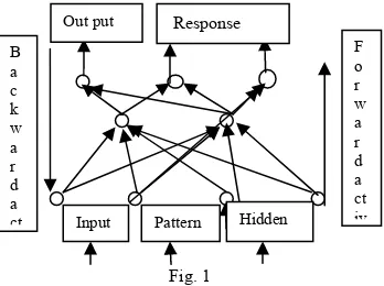
2.1 Error Back – Propagation Algorithms (Back Propagation)
The process of training the network by this method is straight forward as shown in Fig 1. Initially the weights in the network are randomized, except those weights from the outside world to the input layer, which are set as +1. The network, then presented with repeated sets of input patterns together with their correct output patterns
Fig. 1 Out put
Input Pattern
F o r w a r d a ct iv B
a c k w a r d a
ct Hidden
The feed forward operation calculates an output for each input and then compares it with the desired outputs. The difference between the desired and the computed output is the error, and this is then propagated backward through the network using the gradient descent rule (generalized delta rule) to update the weights on the connections as it goes, so that the same error will not occur again. When the error reaches the minimum then the networks has trained.
3. LITERATURE REVIEW –ARTIFICIAL NEURAL NETWORKIN G
Over the last decade, artificial neural networks (ANNs) have been applied to many geotechnical problems such as prediction of soil behaviour, earth retaining structures, slope stability, pile capacity, swelling behaviour, estimation of shear strength etc. [3]. The growing interest in neural networks among researchers is due to their excellent performance in modelling nonlinear multivariate relationships. A neural network is a computational mechanism able to acquire, represent, and compute a mapping from one multivariate space of information to another, given a set of data representing that mapping. (Garrett 1994).[6, 7, 9]
Artificial neural networks (ANNs) (Fausett 1994; Flood and Kartam 1994; Hecht-Nilsen 1990; Maren et al. 1990; Zurada 1992) are a form of artificial intelligence, which, in their architecture, attempt to simulate the biological structure of the human brain and nervous system. ANNs have been applied extensively too many prediction tasks, as they have the ability to model the nonlinear relationship between a set of input variables and the corresponding outputs[6, 8, 10, 23].
Penumadu et al (1994) Model the stress strain behaviour of clay, incorporating rate dependent behaviour using Artificial Neural Network. The prediction is consistent with the observed rate dependent behaviour of soil [16]. Ellis et. al. (1995); have attempted to model Stress – Strain Relationship of sands with varying grain size distribution and stress history using Artificial Neural Networks. In this, investigation authors confirmed that a sequential ANN with feedback is more effective than a conventional ANN without feedback, to simulate the stress strain relationship of soil[4]. Shang, et al (2004); developed Artificial Neural Networks model to capture the multi-variable relationship between the complex permittivity and the soil properties such as density, water content, and degree of saturation. Three ANN models have been developed to the prediction for soil water content, for the degree of saturation, and for the dry density of soil. Authors concluded that the models have appropriate architectures, reasonable complexities, and reliable performance. [19]
ANN modelling on sand and gravel had also been studied by Dayakar Penumadu and Rongda Zhao (1998). They have carried out an extensive ANN model to predict stress strain and volume behaviour of sand and gravel (Triaxial compression behaviour) with effect of mineralogy, grain shape, and size distribution, void ratio and confining pressure. They observed behaviour in terms of nonlinear stress-strain relation, compressive volume change at low stress levels, and volume expansion at high levels are capture well by these models. [17]
Mohamed A. Shahin et al. (2002); developed a model to predicting settlement of shallow foundations on cohesion less soil using neural networks. They observed that results indicate that ANNs are a useful technique for more accurate settlement prediction of shallow foundation on cohesionless soils. [15]
The investigation carried out by the A. Burak et al. (2008) has established correlation between index
properties and shear strength parameters of normally consolidated clays by statistical and neural approaches. They have reported that the results indicate that the ANN-based model is superior in determining the relationships between index properties and shear strength parameters than the statistical. [1]Sinha, et al. (2007), have proposed Artificial Neural Network prediction models that relate permeability, maximum dry density (MDD) and optimum moisture content with classification properties of the soil. Authors had reported that predictions with in 95% confidence interval could obtain from the ANN models. [18]
Najjar, et al. (2007); developed a recurrent neuronet approach to simulate the effect of loading rate and stress history on clay response. The predicted response showed that the developed neuronet-based model was successfully able to qualitatively assess the impact of strain rate and stress history on clay behaviour. [15].
Musharraf, et al (2010); developed a neural network modelling of resilient modulus, MR using routine subgrade soil properties. The strength and weakness of the developed models are examined by comparing the predicted MR values with the experimental values with respect to the R2 values. Overall, the MLPN model with two hidden layers compared to LN, GRNN, and RBFN was found to be the best model for predict resilient modulus. [22]
Saini Sangita, et al (2010); developed an ANN model to predict of skin penetration. The correlation between the skin permeability coefficient and the Abraham descriptors were obtained from the trained neural network. [20].
4. SOURCE AND CHARACTERISTICS OF SOIL –
The soil sample for study was collected from Vidisha city in M.P. state of India. The soil is fine grained and is classified as CI i.e. clay of medium plasticity and compressibility as per IS 1498-1970. The soil contains about 43.6% sand. The soil is expansive in nature. The particle size and index properties of the soil are given in Table 1.
Table 1: Basic properties of the soil.
LL= Liquid limit, PL = Plastic limit, PI= Plasticity index, DFS= Differential swell pressure, G= Specific gravity.
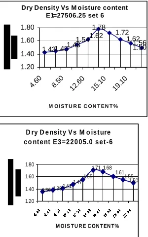
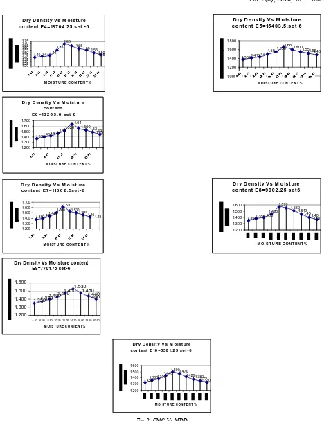
5. COMPACTION TESTS –
Compaction testing determines the optimum moisture content to achieve the maximum dry density under a designated compactive effort for a specific soil. The density of soil is an important parameter since it controls the shear strength, bearing capacity, compressibility and permeability.Total 10 sets of experiments were performed with varying compacting energy.
Dry Density Vs M o isture content E1=27506.25 set 6
1.72 1.62
1.56 1.50 1.78
1.62 1.48 1.45 1.43
1.54
1.20 1.40 1.60 1.80
4.60 8.50 12.60 15.10 19.10
M O I ST U R E C O N T EN T %
D ry D e ns it y V s M o is t ure c o nt e nt E 2 =2 4 2 0 5 .5 s e t 6
1.52 1.58 1.52
1.41 1.42 1.45 1.57
1.74 1.66 1.61
1.20 1.40 1.60 1.80
M oi s t ur e c ont e nt %
D ry D e ns it y V s M o is t ure c o nte nt E 3 =2 2 0 0 5 .0 s e t -6
1.50 1.55 1.47
1.36 1.381.41 1.55
1.71 1.68 1.61
1.20 1.40 1.60 1.80
M OI S TU R E C ON T EN T%
% silt & clay % fine sand 75μ-2 mm % coarse sand 2-4.75 mm LL % PL % PI DFS. % G
D ry D e ns it y V s M o is t ure c o nt e nt E 4 =18 7 0 4 .2 5 s e t - 6
1.65 1.59 1.55 1.50 1.45 1.69 1.44 1.42 1.40 1.55 1.20 1.25 1.30 1.35 1.40 1.45 1.50 1.55 1.60 1.65 1.70 1.75
M OI S T U R E C ON T EN T %
D ry D e ns it y V s M o is t ure c o nt e nt E 5 =15 4 0 3 .5 .s e t 6
1.55 1.600 1.66 1.48 1.52 1.550 1.43 1.410 1.380 1.50 1.000 1.200 1.400 1.600 1.800
M OI ST U R E C ON T E N T %
D r y D ensi t y V s M o i st ur e co nt ent
E6 =13 2 0 3 . 0 set 6
1.45 1.49 1.53 1.560 1.64 1.520 1.420 1.3701.400 1.47 1.200 1.300 1.400 1.500 1.600 1.700
M OI ST U R E C ON T E N T %
D r y D ensi t y V s M o i st ur e co nt ent E 7=110 0 2 . 5set - 6
1.46 1.43 1.500 1.530 1.610 1.440 1.400 1.380 1.500 1.200 1.300 1.400 1.500 1.600 1.700
M OI ST U R E C ON T E N T %
D ry D e ns it y V s M o is t ure c o nt e nt E 8 = 9 9 0 2 .2 5 s e t 6
1.550 1.510 1.45 1.37 1.40 1.570 1.400 1.380 1.350 1.460 1.200 1.300 1.400 1.500 1.600
M OI S T U R E C ON T EN T %
Dry Density Vs M oisture content E9=7701.75 set-6 1.400 1.440 1.480 1.530 1.480 1.400 1.370 1.350 1.430 1.200 1.300 1.400 1.500 1.600
4.40 6.20 8.50 10.20 12.00 14.10 16.00 18.20 20.50 M OI S T U R E C ON T EN T %
D r y D ensit y V s M o i st ur e co nt ent E10 =550 1. 2 5 set - 6
1.330 1.420 1.470 1.350 1.380 1.500 1.390 1.360 1.330 1.440 1.200 1.300 1.400 1.500 1.600
M OI ST U R E C ON T E N T %
Fig. 2: OMC Vs MDD
7701.75 and 5501.25 K.cal. The water content and the weight of the sample required to fill the mould are determined. Results have been plotted as dry density versus water content as shown in Fig 2.
5.1 - Unconsolidated-Undrained (UU or Q Test) -
One of the most important design input parameters needed for geotechnical design is soil’s shear
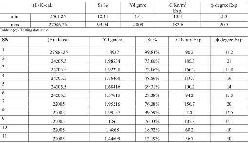
strength. The shear strength is commonly defined by the Mohr-Coulomb failure envelope; τ = σn tan ф + c where, τ = Shear strength, σn = Normal stress, ф = Angle of shearing resistance and c = cohesion. In the present work, soil sample of a set i.e. for a particular compactive effort were prepared at dry of optimum, wet of optimum and at optimum moisture content. Thus in all for 10 sets S1-S10 total 198- samples were tested. The diameter and height of samples were 38 mm. and 76 mm. as per IS 2720 part XI. The prepared samples were saturated and then tested in triaxial test under UU condition. Cell pressure σ3 in the range of 1.0 kg/ cm2, 1.5 kg/ cm2 and 2.0 kg/cm2 have been applied in the chamber by pressurizing the cell fluid (water). Under a particular cell all pressure, vertical stress was increased by loading the specimen until shear failure occurs. Measurement of σd, axial deformation, and sample volume change are recorded. From deviator stress v/s axial strain plot the peak deviator σdf was found. The major principal stress is σ1 = σdf + σ3. Plot Mohr circle that is, based on σ1 and σ3 at failure for different σ1 and σ3 values and make a straight line, which was tangent to all Mohr’s circles. This gives ‘C’ the intercept at y – axis and ф the inclination of this line to the horizontal. As mentioned earlier total 198 test results are available, out of which 120 have been used to train the model, 39 have been used to validation the model and 39 are used for testing. Minimum- maximum values of training , validation data’s and input values – output results of testing data’s are given in Table 2 (a), 2 (b) 2 (c) and 2 (d) respectively.
Table 2 (a) - Training data set -
(E) K-cal. Sr % Yd gm/c C Kn/m2 Exp. ф degree Exp
min. 5501.25 12.01 1.43 25.8 6.4
max 27506.25 99.99 2.09 190.2 21.3
Note: Compaction Energy – E, Degree of Saturation – Sr- %, Dry density – Yd, Cohesion (measured) – C, and Angle of friction ( measured) – ф. Cohesion (predicted) – C’, and Angle of friction (predicted) – ф’
Table 2 (b) - Validation data set: -
(E) K-cal. Sr % Yd gm/c C Kn/m2
Exp.
ф degree Exp
min. 5501.25 12.11 1.4 15.4 5.5
max 27506.25 99.94 2.009 182.6 20.5
Table 2 (c) - Testing data set -:
SN (E) - K-cal. Yd gm/cc Sr % C Kn/m2Exp. ф degree Exp
1 27506.25 1.8937 99.83% 90.2 11.2
2 24205.5 1.98534 73.60% 185.3 21
3 24205.5 1.92228 72.06% 166.2 19.8
4 24205.5 1.76468 48.86% 119.7 16
5 24205.5 1.68416 39.31% 100.2 14
6 24205.5 1.57615 28.38% 94.2 12.5
7 22005 1.95216 76.38% 156.7 20
8 22005 1.99157 99.59% 121 16.5
9 22005 1.86 76.33% 105.3 15.1
10 22005 1.4868 18.72% 60.2 10
12 18704.25 1.8631 77.09% 105.3 15.1
13 18704.25 1.89225 99.51% 80 11.5
14 15403.5 1.9561 99.99% 100.1 14.5
15 15403.5 1.653 35.98% 87.7 13
16 13203 1.7603 69.82% 75.5 12
17 13203 1.4854 18.42% 60.2 10
18 13203 1.84265 99.49% 51.2 9
19 11002.5 1.80336 60.49% 105.7 16.3
20
11002.5 1.8018 63.86% 112.4 15
21
11002.5 1.6665 39.15% 82 13.7
22
11002.5 1.5696 28.91% 85 12.2
23 11002.5 1.84782 99.27% 50 9
24 9902.25 1.7918 59.54% 110.4 15.5
25
9902.25 1.8634 99.96% 50 9.5
26
9902.25 1.8592 99.05% 47.3 9.5
27
9902.25 1.84265 99.49% 35.6 8.4
28
7701.75 1.91068 99.48% 73.8 12
29
7701.75 1.8864 99.58% 64.6 11
30
7701.75 1.8634 99.96% 50 9.5
31
7701.75 1.8306 99.55% 20 7.5
32
7701.75 1.83195 99.83% 20 7.5
33
5501.25 1.87582 99.97% 66.8 11
34
5501.25 1.8492 99.56% 38.3 9
35
5501.25 1.45792 20.45% 40 10
36
5501.25 1.64025 60.12% 28.2 8
37
5501.25 1.82925 99.27% 20 7.5
38 5501.25 1.3965 13.56% 19.4 7
39 5501.25 1.81944 99.80% 15 5.5
SN. Predicted C
by ann -lm Predicted phi by ann -lm Predicted C by ann -rb Predicted phi by ann -rb
1 90.19288 11.54864 96.6 13.5
2 184.6365 20.85117 198 24.6
3 165.7501 19.49457 145.7 16.4
4 115.2276 17.65149 102.3 13.2
5 81.4871 14.47871 88.9 12.7
6 116.0657 10.56361 102.5 15.6
7 156.3761 18.58961 143.4 22.7
8 120.9479 16.33617 139.7 18.9
9 105.2793 14.31879 98.3 17.8
10 60.63413 9.992169 70 7.3
11 56.52804 9.996487 71.6 12.4
12 105.242 14.6831 100 15
13 79.58474 12.02929 88.3 14.8
14 102.5833 14.0273 90.7 12.4
15 87.38011 13.05155 76.9 11.2
16 74.79625 12.23971 87.2 10.7
17 60.36698 10.19894 54.2 7.3
18 51.45235 9.386785 45.2 11.7
19 105.4196 16.07576 100.3 14
20 100.3676 15.62574 126.8 10.3
21 81.89722 14.03023 98.3 16.3
22 84.80888 12.01478 82.5 12.4
23 48.61404 9.210888 53.2 8.7
24 105.1044 15.80045 119.2 13.1
25 53.54179 9.814599 63.2 12.3
26 44.52102 9.317167 34.7 7.8
27 34.33533 8.120606 30.2 7.3
28 70.14635 12.27809 87.3 10
29 61.62939 11.2674 78.3 13.7
30 49.99618 9.930739 38.8 12.3
31 16.22408 6.707084 18 7.3
32 18.09615 6.854341 27.3 8.3
33 58.09392 10.87879 65.5 10.7
34 42.02271 9.134603 33.3 10.7
35 39.58166 9.871288 44.7 8
36 27.34591 7.875312 20.2 9
37 22.75835 7.308468 17.4 6.3
38 19.33103 7.191239 23.8 8.4
39 12.27302 6.378325 14.2 6.2
Radial Basis Function Network-
The radial basis function network divides the modeling space using hyper spheres. To trained the networks 120 dataset out of 198 have used as training data, 39 dataset as validation and 39 dataset for testing the networks with three nodes of input parameters. In present architecture variable input parameters has taken for training is compaction energy, degree of saturations and dry density. That type of network model has one hidden layer. In the present training model, optimum numbers of neurons found to be 42, by trial and error method. The cohesion and angle of friction are two output nodes.
Fig 3 - Radial Basis Function architecture
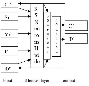
Multilayer layer perceptron network-
The software MATLAB-7.0 was used to make architecture of 5-35-30-40-02 was trained on 120 triaxial test results validation on 39 and testing on 39 test results. In present architecture, three input variables compaction energy, degree of saturation, dry density and two outputs cohesion and angle of internal friction has taken for training. The current state values of outputs as an inputs are C” and ф”. The outputs are C” and ф” these value is equal to the network feed forward computation of the input values Yd up to last iteration. In the hidden layer the processing elements was determined through a trial and error method. An adaptive learning rate and momentum factors have been used wherever the connection weights updated. For each trial no. of hidden layer modes, random initial weights & biases are generated. The neural network is then trained with different combinations of momentum terms and learning rules in an attempt to identify the ANN model that performs best testing data.
The momentum terms used in this study are 0.8, whereas the learning rates used are 0.0000001, since the back propagation training algorithm uses a first order gradient descent technique to adjust the connection weights. Different
Sr
Yd
E
C’
Ф
’
3
5
N
eu
ro
ns
H
id
de
Ф
”
C”
Input 3 hidden layer out put
Fig. 4 - ANN architecture 3 0 n e u r o n s
4 0 n e u r o n
E
Sr
Yd
42
Neu
rons
C’
initial weights were used at the start of the training and the network did coverage to vary similar predictions. ANN architecture is shown in Fig. 4.
5.3 – Comparison of Testing data set –
The results or output obtained from MLPN model, RBN model have been compared with experimental results of cohesion and angle of internal friction and are shown in graph. Fig 5 [a] [b] [c] and [d].
0.1 0.2 0.3 0.4 0.5 0.6 0.7 0.8 0.9 1 0
20 40 60 80 100 120 140 160 180 200
Sr Vs Cohesion
Sr
C
ohes
ion
measured cohesion predicted ann by lm predicted ann by rbfn
1.3 1.4 1.5 1.6 1.7 1.8 1.9 2 0
20 40 60 80 100 120 140 160 180 200
Yd Vs Cohesion
Yd
Co
h
e
s
io
n
measured cohesion predicted cohesion ann by lm predicted cohesion ann by rbfn
0.1 0.2 0.3 0.4 0.5 0.6 0.7 0.8 0.9 1 5
10 15 20 25
Sr Vs Phi
Sr
Ph
i
measured phi predicted phi ann by lm predicted phi ann by rbfn
1.3 1.4 1.5 1.6 1.7 1.8 1.9 2 5
10 15 20 25
Yd Vs Phi
Yd
Ph
i
measured Phi predicted phi ann by lm predicted phi ann by rbfn
Fig.5(c)(d)Comparision of experimental and predicted angle of friction
6. RESULTS AND DISCUSSION –
The objective of this study was to make a predictive model to correlate the compaction energy, degree of saturation and dry density values of high compressible soil with shear strength parameters, cohesion and angle of internal friction. A database was developed, containing Atterberg limits –liquid and plastic limit, grain size distribution, specific gravity, standard proctor and unconsolidated undrained triaxial results for 198 number of test. From the experimental samples, 120 soils data base were used in training, 39 soils data were used in validation and 39 soils data used in testing the MLPN and RBFN ann model. Commercial software, MAT LAB-7.0, was used to develop predictive models.
REFERENCES:-
[1] Burak Goktepe A., Selim Altun, Gokhan Altintas and Ozcan Tan, “Shear strength estimation of plastic clays with statistical and neural approaches”, Journal of Building and Environment, 2008, vol. 43, issue 5, pp. 849-860
[2] Basarkar S, “Neural Network Applications in Geotechnical Engineering soft computing”, conf. proceeding of Soft computing in civil engg. 2006, I.I.T Bombay.
[3] Dihoru, L. et. al “ A neural network for error prediction in a true triaxial apparatus with flexible boundaries”, Computers and Geotechnics, 2005, vol. 32, pp. 59-71.].
[4] Ellis G. W., Yao,C. Zhao R., and Penumadu,D. “Stress-strain modeling of sand using artificial neural network”, Journal of geotechnical engineering, 1995, ASCE, vol. 121, no. 5, pp. 429-435.
[5] Freeman A., David M. Skapura, “Neural Network, Algorithm, Application and Programming Techniques”, James - Pearson Education Asia.
[6] Flood, I. and Kartam, N.C. “Neural Network in Civil Engineering-2 Principles and understanding” ASCE journal of computing in Civil Engineering, 1994, vol.8, no.2, pp.149-162.
[7] Faghri, A., Marthinelli, D., and Demetsky, M. J, “Neural Network Applications in Transportation Engineering”, in Artificial Neural Networks for Civil Engineers Fundamentals and Applications, Kartam, N., Flood, I., and Garrett, J.H., Jr., eds., Expert Systems and Artificial Intelligence Committee, ASCE, 1997, Chapter 7.
[8] Fausett, L.V. “Fundamental of neural networks: Architecture, algorithem, and applications”, 1994, Prentice-Hall, Inc., Englewood Cliffs, N.J.
[9] Garrett, J.H., “Where are why Artificial Neural Network are applicable in Civil Engineering journals of computing in Civil Engineering”, 1994, ASCE, vol. 8, no. 2, pp. 129-130.]
[10] Hecht-Nielsen, R. “Neurocomputing.Addison-Wesley, Boston, Mass, 1990.
[11] Isik, N. S. “Estimation of swell index of fine grained soils using regression equations and artificial neural networks”, Scientific Research and Essay, 2009, Vol.4 (10), pp. 1047-1056.
[12] Indian Standard methods of “determination of the unconsolidated undrained triaxial shear test”, IS: 2720 (Part XI) -1971
[13] Mohd Jamal, Mohd Amin,.Raihan Taha, et al., “Prediction and Determination of Undrained Shear Strength of Soft Clay at Bukit Raja, Pertanika”, J. Sci & Technol, 1997, vol. 5, no. 1. pp. 111-126].
[14] Muller, P. & Insua, D. R., “Issues in Bayesian Analysis of Neural Network Models”, Proceedings of Neural Computation, 1998, vol. 10, Issue 3, pp. 749 - 770].
[15] Mohamed A. Shahin, Holger R. Maier, Mark B. Jaksa, “Predicting settlement of shallow foundations using neural networks,” Journal of Geotechnical and Geoenvironmental Engg., 2002, vol. 128, no. 9, pp. 785-793.
[16] Penumadu, Jin Nan, Chameau, and Arumugam, “Rate dependent behavior of clays using Artificial neural network” Proc. 13th Conf. Int.
Soc. Soil mech. & foundation engineering New Delhi, 1994, pp. 1445-1448
[17] Penumadu, and Rongda Zhao, “Triaxail Compression behavior of sand and gravel using artificial neural networks”, Journal of Computer and Geotechnics, 1999, vol. 24, pp. 207-230.
[18] Sinha Sunil K., Mian C. Wang “Artificial Neural Network prediction models for soil Compaction and Permeability”, Journal of Geotech Geol Engg., 2008, vol. 26, pp. 47-64.
[19] Shang J. Q., Ding W and Rowe, R.K. “Soil Characterization using complex permittivity and Artificial Neural Networks”, Journal of Soils and Foundations, 2004, vol. 44, no. 5, pp. 15-26.
[20] Saini Sangita, et al, “Prediction of skin penetration using Artificial Neural Network.” International journal of engineering science and Technology., 2010, vol.2(6), pp. 1526- 1531.
[21] Toll, “Artificial Intelligence Application in Geotechnical Engineering System”, Electronic Journal of Geotechnical Engineering, 1996, vol. 1.
[22] Zaman, M. “Neural network modeling of resilient modulus using routine subgrade soil properties.” Journal of geomechanics, 2010, ASCE, vol. 10, no.1, pp.1-10.