PROGRAMMING APPROACH TO
INVESTIGATE THE EFFECT OF FIELD
VARIABLE FOR NUMERICAL
APPROXIMATION TECHNIQUES
Dr.A.B.Deoghare
Professor, Mechanical Engineering Department,
G. H. Raisoni college of Engineering, Nagpur, Maharashtra, India 440016 [email protected]
AJINKYA PATIL
Research Scholar, Mechanical Engineering Department, St. Vincent Pallotti college of Engineering, Nagpur, India
[email protected] NITIN SAWARKAR
Research Scholar, Mechanical Engineering Department, St. Vincent Pallotti college of Engineering, Nagpur, India
[email protected] KIRAN ZADE
Research Scholar, Mechanical Engineering Department, St. Vincent Pallotti college of Engineering, Nagpur, India
Abstract :
The modern treatment to solve differential equations of problems relies heavily on approximation methods. To keep the discussion simple while maintaining a general formulation of practical interest in engineering, the model problem considered is of an axially loaded bar having quadratic function of area. The unknown variable is the axial displacement of one dimensional continuum, u(x) is attempted in the present research by means of numerical analysis technique where the basic inputs to a problem are known with arbitrary basic data. Numerically evaluating differential and integral is a rather common and usually stable task. Attempting the numerical solution with different approximation methods leads the errors while solving differential equations of the system. A genuine necessity for obtaining precise solution for the different numerical approximation methods is overcome by developing in-house computer program. The developed code is resourceful enough to conquer the calculation result from round-off of arithmetic processes or truncation. The program is interactive and user friendly in operation to change the desired inputs. Graphically results can be displayed to know the effect of considered weights and the constants assumed.
Keywords: Numerical methods; Field variable; MATLAB; Mathematical modeling.
1. Introduction
The governing equations and boundary conditions are useful means to express the mathematical model. In general, engineering problems is often needs to be addressed considering the domain of interest. The differential equations are employed to illustrate the physical significance of the system under the domain of consideration. For such system, analytical solution can be found out using differential equation and boundary conditions. To establish mathematical model it is required to describe the relationships of primary and secondary variables. The solution characteristics can be expressed in the algebraic form. For the well defined simple engineering problems, there are standard known analytical techniques available to find solution. But, there are many engineering problems for which exact solution cannot be easily obtained using analytical techniques. The failure to obtain an exact solution may be attributed to either the complex governing differential equation or the difficulties in dealing with the boundary and initial conditions. To deal with such problems, numerical approximation is best alternative. An approximate technique may become the effective tool to define the nature of unknown variable and enable to determine the solution at discrete points in the problem domain.
In classical method exact equation are formed and exact solution are obtained where as using approximation method exact equation are formed but approximate solution are obtained. Approximate method is useful and easy to used, if it is integrated with computer for the problem involving a number of complexities without making drastic assumption which otherwise complicated to attempt by classical methods.
In the present paper the numerical techniques like Direct Integration, Method of Weighted Residuals, Ritz Method and FEM are used to determine the deviation in the field variable at the selected node position. For this purpose the one dimensional continuum is selected as shown in Fig.1. The computer programming technique is employed to minimize computational cost and time. The developed computer program uses MATLAB tool and developed sets of subroutines and functions. The programs are intended as a primary component for generalization to obtain the results at any position on the continuum. The applications can be extended for variety of similar complex problems.
2. Development of Governing Equations
Consider an axially loaded 1D bar having varying area A with one end fixed at x=0 and externally applied force F at x=L as shown in Fig.1.The free body diagram (FBD) is shown in Fig. 2. The axially loaded continuum considered here has length L=2 m and area as quadratic function of x given by A= 0.01 , E=200 GPa and F=1000 N.
Fig.1 Axially loaded 1D continuum Fig.2 Free body diagram
Governing equation is developed for 1D continuum having varying area. The unknown variable is the axial displacement given by u(x).From the FBD and using equilibrium equation,
0 (1)
Where, A indicates the area which is assumed to be a continuous function with respect to x. The Eq. (1) becomes,
From Hooke’s Law, within elastic limit, Stress Strain [Day, (1964)] [Hildebrand,(1956)]
(3)
Where E is the modulus of elasticity of the system
Substituting inEq. (2)
The governing equation is,
0 , 0 < x <L (4)
There are two boundary conditions associated with the problem,
The essential boundary condition is.
0 0 (5)
and the natural boundary condition,
2 (6) Where F is the axially applied load
3. Development of routine script
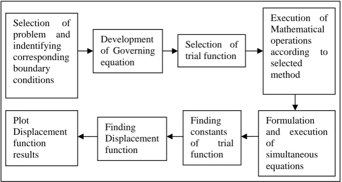
MATLAB provides interactive platform for executing numerical computations. The program code is written in MATLAB 7.10.0 (R 2010a) version. In-house computer program is developed different approximation numerical methods to determine the solutions to overcome long and tedious task which otherwise need to be attempted by hand calculation [Otto, (2005)]. The important steps which are used for writing the program script are indicated in the block diagram shown in Fig 3.
Fig 3 Flow chart representing the steps adopted in writing computer program
Selection of problem and indentifying corresponding boundary conditions
Development of Governing equation
Selection of trial function
Execution of Mathematical operations according to selected
method
Formulation and execution of
simultaneous equations Finding
Displacement function Plot
Displacement function results
4. Approximation Methods
Approximate methods use numerical technique to obtain the solution from the governing equations. The present section discusses the issue of the finding the field variable deviation for the various positions on the continuum. The different standard numerical techniques are applied to these one dimensional continuum systems to determine results at different nodes [Hamming, (1962)].
4.1 Method of Weighted Residuals (MWR)
The weighted residual methods are based on the assumption of an approximate solution for the governing differential equation [Finlayson,(1972)]. The assumed solution must satisfy the initial and boundary conditions of the given problem. As the assumed solution is not exact, substitution of the trial solution into the differential equation will lead to some residuals or errors. Each residual method requires the error to vanish over some selected intervals or at desired points called nodes.
The governing equation for the above considered problem is equal to residual(R) when , where is a polynomial function which describes the solution at the discrete points [Petrolito, (1998)].
The governing equation for these methods is
(7)
Considering trial approximate solution,
= (8)
2 (9)
Applying first B.C. 0 at 0 0
Therefore the Eq. (8) becomes,
= (10)
This function is subsequently used for further calculation.
The weighted residual methods uses virtual work principle and the integrals error function are defined as
0 , 1,2,3 … … … … (11)
0
The equation is integrated by parts
(12)
Where are the weights, which are different for each method.
The constants of trial solution and are calculated by solving Eq. (12) for different weights. The deformation is calculated by substituting them in Eq. (10)
In the developed program the constants are’a1’and ‘a2’ are declared. The letter ‘x’ is variable in ‘u’ of trial solution assumed. The first order differentiation of ‘u’ is calculated as ‘du’. The weights are defined as ‘w1’ and’w2’ which will modify as per the methods considered for analysis. The differentiation of these weights is calculated as ‘dw1’ and ‘dw2’. The differential equation ‘f12’ is formulated by building the equation in terms of ‘f11’. Similarly the second equation ‘f22’ is formulated and integrated over the domain. The integration provides us with two simultaneous equations ‘c1’ and ‘c2’. These equations are solved simultaneously and their values are saved in ‘a’, which is an array holding the solution. The constants of trial solution are retrieved from it and the trial solution is calculated for different values of ‘X’ , the distance of a point from fixed end. The common syntax applicable for the different Method of Weighted Residuals is depicted below with the appropriate comments with each statement.
syms x;
A=(0.01+(0.01*x))^2; % Cross-sectional Area syms a1 a2;
u=(a1*x)+(a2*(x^2));% Trial solution du=diff(u,x);% First differential of u wrt x w1= %**% Weight defined by particular method dw1=diff(w1,x);% First differential of w1 wrt x f11=diff((w1*F),x);% Part 1 of differential eq(1) f12=(dw1*A*E*du);% Part 2 of differential eq(1)
c1=int(f11,x,x1,x2)-int(f12,x,x1,x2);% Total differential eq(1) w2= %**% Weight defined by particular method
dw2=diff(w2,x);% First differential of w2 wrt x f21=diff((w2*F),x);% Part 1 of differential eq(2) f22=(dw2*A*E*du);% Part 2 of differential eq(2)
c2=int(f21,x,x1,x2)-int(f22,x,x1,x2);% Total differential eq(2) a=solve(c1,c2,a1,a2);% Solving eq(1) & (2) simultaneously aa1=a.a1;% Constant 1 of Trial solution
aa2=a.a2;% Constant 2 of Trial solution
uu=(aa1*X)+(aa2*(X.^2));% Equation of Trial solution
The above syntax will remain same only with the changes in the weight used corresponding to the method of selection considered for execution.
4.1.1 Galerkin Method
Galerkin Method is a Weighted Residual Methods which derives its weight functions from the trial solution.
Weight function is given by
1,2,3 … (13)
&
Integral of the error function is Ω . . =0 [Cockburn,(2000)].
Considering the weight functions as & , and finding the constants, the trial solution is obtained. The weights for this method can be calculated in form of
w1_gal=diff(u_gal,a1_gal);% Weight(1)obtained from u w2_gal=diff(u_gal,a2_gal);% Weight(2)obtained from u
The constants are determined and field equation obtained is,
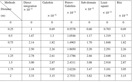
Displacements at various points are determined and represented in Table 1 and the graphically results are represented in Fig 4.
4.1.2 Petrov-Galerkin Method
Petrov-Galerkin Method works on similar approach which uses different pairs of weight functions such as
1& , & , 1& etc.
Considering the weight functions as & for further calculation. The weights for this method can be written in program as
w1_petro_gal=x^2; % First Weight considered w2_petro_gal=x^3; % Second Weight considered
Again the same integral error function is used which is symbolized as
Integral of the error function is Ω . . =0 [Cockburn, (2000)].
The constants are determined and field equation obtained is,
2.353 10 4.8845 10
Displacements at various points is depicted in Table 1 and the graphically results are represented in Fig 4. 4.1.3 Sub domain Method
The domain of Fig.1 is divided in two halves and the analysis is carried out with single weight function [Mikhlin, (1963)].
Considering weight as w= x, 1
The domain is 0 to 2m which is divided into two halves from 0 m to 1 m and 1 m to 2 m. The governing Eq. (12) used in this method which is multiplied by considered weight function. The equation is expressed as
0 (14)
For sub domain 0 to and to Eq. (14) gives two equations which when solved simultaneously provides the constants of trial solution and a2. Additional variable in term of x3=(x2-x1)/2; is defined to indicate intermediate limit of integration.
To execute the program following changes are carried out.
c1=int(f11,x,x1,x2)-int(f12,x,x1,x3);% eq(1) c2=int(f21,x,x1,x2)-int(f22,x,x3,x2);% eq(2)
The constants are determined and field equation obtained is,
=2.4999 10 2.9411 10
4.1.4 Least square Method
The Least Square Method is a weighted residual method which derives its weight functions from the Residual itself [5]. Weight function is given by
1,2,3 … (15)
&
Weights are multiplied with Residual and integrated over the domain [Cockburn,(2000)].
The weights for this method can be calculated in form of
res=diff((E*A*du_les),x); % Residual
w1_les=diff((res),a1_les); % Weight(1)obtained from Residual w2_les=diff((res),a2_les); % Weight(1)obtained from Residual The constants are determined and field equation obtained is,
9.37 10 1.1899 10
Displacements at various points is depicted in Table 1 and the graphically results are represented in Fig 4.
4.2 Ritz Method
In continuum mechanics, a system can be described in terms of an "energy functional", which measures the energy of proposed configuration. It is often impossible to analyze all of the infinite configurations of system with the least amount of energy; an approximate numerical computation is essential [Mikhlin, S. G. (1963)]. Ritz method is applied to the above discussed static equilibrium problem. The trial functions selected above is substituted in to the functional. The is equal to summation of strain energy and applied work potential. Functional governing equation is
(16)
Now differentiate Eq. (16) with constants of trial function ,
0 (17)
0 (18)
Solving simultaneous Eq. (17) and Eq. (18) the constants are determined and field equation obtained is ,
2.9452 10 6.8493 10
Displacements at various points is depicted in Table 1 and the graphically results are represented in Fig 4.
4.2.1 Program code for Ritz method
syms x a1 a2
u=(a1*x)+(a2*(x^2));% Trial solution du=diff(u,x);% First differential of u wrt x
p1=(0.5*E*A*(du^2));% Part 1 of Pi inside function ulr=((a1*x2)+(a2*(x2^2)))*R;% Part 2 of Pi function p2=int(p1,x,x1,x2);% Part 1 of Pi final function pi=p2-ulr;% Total Pi function
d1pi=diff(pi,a1);% First differential of pi wrt a1 eq(1) d2pi=diff(pi,a2);% First differential of pi wrt a2 eq(2)
a=solve(d1pi,d2pi,a1,a2);% Solving eq(1) & eq(2) simultaneously a1=a.a1;% Constant 1 of Trial solution
a2=a.a2;% Constant 2 of Trial solution
uu=(a1*X)+(a2*(X.^2));% Equation of Trial solution
Executing the program the displacements at various points is depicted in Table 1 and the graphically results are represented in Fig 4.
5 Direct Integration Approach
The direct integration technique is analytical way of finding exact solution [Pian (1969)].
The result of approximate method is verified using classical methods i.e. Direct Integration method.
The technique is used for obtaining the result and finding the error of field variable at the discrete points.
Applying boundary condition, 0 0
Substituting values of F, E and A at x=2 and applying 2nd boundary condition Equation 6 becomes
(19)
Integrating the governing equation (4),
(20)
. (21)
Again Integrating,
. (22)
Now, applying 2nd boundary condition to Eq. (20) i.e substitute x=2, the result is 1000
Put the value of in Eq. (22) at x=0,
5 10
Substituting the value of and in Eq. (21), the generalized equation for displacement is,
The displacement at interval of 0.25 m increment position from the starting point is evaluated and depicted in Table 1 and the graphically results are represented in Fig 4.
5.1 Program code for Direct Integration method.
The developed program calculate‘c1’ and ‘c2’, the constants of the governing differential equation. The deformation is calculated in three statements of program. ‘X’ is an array having different values of distances from fixed end. The second step call the value of X and final deformation values are obtained in the third step.
F=input('Enter load acting on body in "N":-');
E=input('Enter the value of Youngs modulus in "GPa":-'); E=E*(10^9); % to convert in GPa
x1=input('The starting position of deformation in "m":-'); x2=input('The ending position of deformation in "m":-'); n=input('The number of parts the body is to be divided:-'); X=x1:(x2/n):x2; % produces array of distance from fixed end du=(R/(E*((0.01+(x2/100))^2)));% First differential of u wrt x c1=(du*(E*((0.01+(x2/100))^2)));% Constant of integration 1 c2=(100*c1/(E*(0.01)));% Constant of integration 1
k1e=(E*(0.01+(X/100)))/(-100*c1); k2e=k1e.^(-1);
ue=(k2e) + c2;% Equation of deformation
Table 1 deformation results for the numerical methods considered
Methods Distance (m)
Direct integration
10
Galerkin
10
Petrov-Galerkin
10
Sub-domain
10
Least square
10
Ritz
10
0 0 0 0 0 0 0
0.25 1 0.69 0.5578 0.60 0.703 0.69
0.5 1.67 1.3 1.0546 1.17 1.319 1.3
0.75 2.14 1.82 1.4903 1.70 1.848 1.82
1 2.50 2.26 1.8650 2.20 2.291 2.26
1.25 2.78 2.61 2.1786 2.66 2.648 2.61
1.5 3.00 2.87 2.4311 3.08 2.918 2.87
1.75 3.18 3.05 2.6226 3.47 3.101 3.05
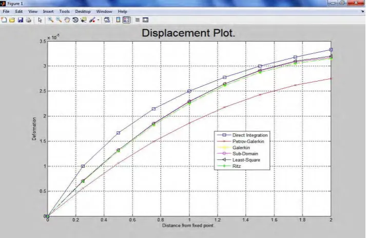
Fig 4 Displacement plot for the considered continuum
The displacement plot indicates that the “Sub Domain” and “Least Square Method” gives more precise results in the interval of 0 to 1 m and 1 to 2 m respectively. The graph shows maximum deviation of the field variable in the initial and extreme phase for the Petrov- Galerkin, while the result of Ritz and Galerkin is same for the quadratic function of area. The trend is observed almost for all the methods when compared with direct integration method [Hughes, (2000)].
The percentage error is calculated with respect to direct integration method and it is represented in Table 2. Table 2 Percentage error in deformations
Methods Galerkin
Petrov-Galerkin
Sub-domain Least square Ritz
Distances(m) 0 m
0 0 0 0 0
0.25 30.70 44.20 29.4 29.74 30.7
0.5 21.90 36.80 20.5 20.88 21.9
0.75 14.80 30.35 13.4 13.75 14.8
1 9.60 25.40 8.24 8.35 9.60
1.25 6.011 21.63 4.7 4.68 6.01
1.5 4.10 18.96 2.9 2.74 4.10
1.75 3.90 17.52 2.9 2.53 3.90
6. Conclusions
The issue of selecting the numerical methods to obtain the approximate solution for the system is addressed with different numerical approximation methods. The weighted residual methods explicitly include the errors in the field variable which is found out using the developed program. Fine variation in the field variable is possible with the developed program by using the desired steps of increments. The best convergence is found out by executing these numerical techniques to select the appropriate regions of operations. The smooth convergence close to the exact solution is essential for a best possible selection of trial solution which is possible with the developed program. Selection of trial function can be forecasted based on the results of field variable error percentage. The computer programming technique is employed to minimize computational cost and time.
References:-[1] Ames,W. F. (1992).Numerical Methods for Partial Differential Equations, 3rd edn, Academic Press, New York,.
[2] Cockburn, B.; Karniadakis, G.E. and Chi-Wang Shu (2000). Discontinuous Galerkin Method: Theory, Computation and applications. Springer-Verlag, Berlin.
[3] Day, J.T.; and Collins, G.W. (1964), "On the Numerical Solution of Boundary Value Problems for Linear Ordinary Differential Equations", Comm. A.C.M. 7, pp 22-23.
[4] Finlayson, B. A. (1972).The Method of Weighted Residuals and Variational Principles, Academic Press, New York,.
[5] Hamming, R.W. (1962) "Numerical Methods for Scientists and Engineers" McGraw-Hill Book Co., Inc., New York, San Francisco, Toronto, London, pp. 204-207.
[6] Hildebrand, F.B. (1956), "Introduction to Numerical Analysis" McGraw-Hill Book Co., Inc., New York, Toronto, London, pp. 258-311.
[7] Hughes,T.J.R.; Angel,G.; Mazzei,L. and M.G. Larson (2000). A comparison of discontinuous and continuous Galerkin method based on error estimates, conservation, robustness and efficiency. In discontinuous Galerkin method: Theory, Computation and application, Springer-Verlag, Berlin, pp.135-136.
[8] Marquardt, D.W. (1963),"An Algorithm for Least-Squares Estimation of Nonlinear Parameters", J. Soc. Ind. Appl. Math., Vol.11, No. 2, pp.431-441
[9] Mikhlin, S. G. (1963). Variational Methods in Mathematical Physics, Pergamon Press, New York,.
[10] Otto S.R. and Denier J.P. (2005), An Introduction to Programming and Numerical Methods in MATLAB. Springer-Verlag, Berlin. [11] Petrolito, J. (1998). Approximate solutions of differential equations using Galerkin’s method and weighted residuals, Australia.
pp.14-25.