POTENTIAL ROLE OF MARINE SNOW IN THE FATE OF SPILLED OIL IN COOK INLET, ALASKA

(1)

University of New Hampshire University of New Hampshire

University of New Hampshire Scholars' Repository

Master's Theses and Capstones Student Scholarship

Winter 2019

POTENTIAL ROLE OF MARINE SNOW IN THE FATE OF SPILLED

OIL IN COOK INLET, ALASKA

Jesse Ross

University of New Hampshire, Durham

Follow this and additional works at: https://scholars.unh.edu/thesis

Recommended Citation Recommended Citation

Ross, Jesse, "POTENTIAL ROLE OF MARINE SNOW IN THE FATE OF SPILLED OIL IN COOK INLET, ALASKA" (2019). Master's Theses and Capstones. 1331.

https://scholars.unh.edu/thesis/1331

This Thesis is brought to you for free and open access by the Student Scholarship at University of New Hampshire Scholars' Repository. It has been accepted for inclusion in Master's Theses and Capstones by an authorized administrator of University of New Hampshire Scholars' Repository. For more information, please contact

(2)

POTENTIAL ROLE OF MARINE SNOW IN THE FATE OF

SPILLED OIL IN COOK INLET, ALASKA

By

JESSE ROSS

Bachelor of Science, Environmental Engineering, University of New Hampshire, 2017

THESIS

Submitted to the University of New Hampshire

in Partial Fulfillment of

the Requirements for the Degree of

Master of Science

In

Civil and Environmental Engineering

(3)

(4)

iii This thesis has been examined and approved by:

Dr. Nancy Kinner, Thesis Director

Professor of Civil Engineering and Environmental at the University of New Hampshire

Dr. Kai Ziervogel, Co-Advisor

Research assistant professor of Oceanography at the University of New Hampshire

(5)

iv Original approval signatures are on file with the University of New Hampshire Graduate School.

ACKNOWLEDGEMENTS

This research was made possible by the support and funding of the University of New

Hampshire (UNH) Coastal Response Research Center (CRRC), Cook Inlet Regional Citizens

Advisory Council (CIRCAC), and the National Oceanic and Atmospheric Administration

(NOAA).

I would like to thank Dr. Nancy Kinner for many years of consistent support, perspective,

and willingness to invest time in me. Nancy’s unwavering energy, curiosity, work-ethic, and

passion is contagious. Thanks for pushing us all towards achieving more, while reminding us to

“let go” of what we do not need.

I would like to thank Dr. Kai Ziervogel for thoughtfully introducing an engineering student

to the world of oceanography. His genuine excitement about understanding the underlying

mechanisms of the environment changed the way I approached laboratory work.

I’d like to thank Susan Saupe (CIRCAC Director of Science & Research) and everyone at

CIRCAC for funding this project. This project would not have been possible without Sue’s

extensive experience, ability to make things happen, and knowledge, along with her willingness

to be a mentor throughout.

Thank you to Melissa Gloekler for being a great friend. Thanks to Kathy Mandsager for

(6)

v of what CRRC does. You both made it possible to truly enjoy this process. Thank you to all the

ERG folks who make Gregg a special place to work.

Thanks to skippers Hans Pedersen (University of Alaska Fairbanks) and Mike Geagel

(NOAA) for incredible seasons in Kachemak Bay. Thanks to Connie Geagel (UAF), Dominic

Hondolero (NOAA), and Kris Holderied (Director of Kasitsna Bay Lab, NOAA), for their support

of this research in so many ways. You all made this project and experience successful and fun.

Thanks to all who served on the Project Advisory Committee: Susan Saupe (CIRCAC),

Kris Holderied (NOAA), Dr. Sarah Allan (NOAA), Cathy Coon (BOEM), Catherine Berg

(NOAA), and Dr. Rick Bernhardt (AK DEC).

Thanks to Dr. Tom Ballestero for serving on my committee. Thanks to Dr. Phil Ramsey

for his thoughtful time helping with statistical analysis.

Thanks to so many friends who have helped from the field to the lab: Dr. Alexandra Ravelo,

Maya Thompson, Jim Schloemer, Mikie Geagel, Kim Shuster, Quinn Wilkins, Peter Saunders,

Katie McCabe, Bryan Zhang, and the crew of the M/V Miss Diane. Also, thanks to my friend

Wiley Little for friendship and patience.

Finally, I’d like to thank my family: Abby, for setting a life-long inspiring example of hard

work and integrity, and my parents for selflessly giving so much energy, love and support.

(7)

vi

LIST OF TABLES

Table 2.1 Experimental set-up for roller-bottle incubations ... 20

Table 3.1 Sample replicates from all events from June 2018 to July 2019 ... 30

Table 3.2 Summary of TPM and TVS fluxes ... 31

Table 3.3 Mean concentrations of suspended matter at the depth of the trap by site ... 32

Table 3.4 Summary of surface water at start of each incubation by start date ... 52

Table 3.5 Qualitative observations of oil-related marine snow incubations ... 53

Table 3.6 Results summary TPM and TVS means from all three experiments ... 58

Table 3.7 Connecting letters report of upper bottle TPM across treatments ... 58

(10)

ix

LIST OF FIGURES

Figure 1.1 Labeled satellite image of Cook Inlet and Western Gulf of AK ... 9

Figure 2.1 Map of lower Cook Inlet showing sites of sediment trap deployments. ... 14

Figure 2.2 A schematic of the surface-tethered sediment trap assembly ... 16

Figure 2.3 All bottles prior to rolling ... 21

Figure 2.4 The six sites sampled on the July 2019 cruise. ... 25

Figure 3.1 Density profiles of the upper 25 m of the water column ... 28

Figure 3.2 Bar graph showing TPM (Blue) with TVS (Red) with standard error bars ... 31

Figure 3.3 Mean Copper River discharge in 2018 to 2019 ... 34

Figure 3.4 Surface current speeds (knots) at maximum flood ... 37

Figure 3.5 Drift Distance over Time vs. Time from Slack by Site ... 38

Figure 3.6 Mean Settling Velocities per Tube vs. Site by Year ... 40

Figure 3.7 Photomicrographs of filtered contents... 41

Figure 3.8 Video screenshots of pelagic species at trap depth. ... 43

Figure 3.9 Density profiles with depth across Albatross (upper) and Portlock (lower) Banks .... 47

Figure 3.10 Fluorescence profiles with depth ... 48

Figure 3.11 Mean and standard error of TPM and TVS fluxes ... 49

Figure 3.12 Box plots of mean particle sinking velocities vs. Sitet. ... 50

Figure 3.13 Photographs of each treatment following Experiment 3 ... 53

Figure 3.14 Photomicrographs of each condition. ... 54

Figure 3.15 Oil content was estimated by comparing binary areas. ... 55

Figure 3.16 All TPM and TVS values for each incubation ... 56

(11)

x

LIST OF ACRONYMS

BOEM: Bureau of Ocean Energy Management

CIRCAC: Cook Inlet Regional Citizens Advisory Council

CRRC: Coastal Response Research Center

DWH: Deepwater Horizon

EVOSTC: Exxon Valdez Oil Spill Trustee Council

EPS: Extracellular Polymeric Substances

TEP: Transparent Exopolymer Particles

GoMRI: Gulf of Mexico Research Initiative

GF/F: Glass Fiber Filter

ACC: Alaskan Coastal Current

CTD: Conductivity Temperature Depth

GoA: Gulf of Alaska

GoM: Gulf of Mexico

KB: Kachemak Bay

MOSSFA: Marine Oil Snow Sedimentation and Flocculant Accumulation

NERR: National Estuarine Research Reserve

NMS: Natural Marine Snow

NOAA: National Oceanic and Atmospheric Administration

OMA: Oil-Mineral Aggregate

ORMS: Oil-Related Marine Snow

PSU: Practical Salinity Unit

(12)

xi TPM: Total Particulate Matter

TVS: Total Volatile Solids

(13)

xii

ABSTRACT

POTENTIAL ROLE OF MARINE SNOW IN THE FATE OF SPILLED OIL IN COOK INLET, ALASKA

By

Jesse Ross

University of New Hampshire, December 2019

While extensive research has been conducted on minerals aggregating with spilled oil,

surface-forming organic aggregates, called marine snow, have only recently been studied as a

transport mechanism. This knowledge gap in understanding the fate of oil was highlighted

following the 2010 Deepwater Horizon (DWH) blowout in the Gulf of Mexico when a significant

percentage of the spilled oil reached the seafloor as a result of association with marine snow.

Research following the DWH blowout suggests both marine snow and mineral aggregates are

significant oil exposure pathways that must be considered during an oil spill response. The U.S.

Geological Survey and others have noted that understanding particle fluxes in areas of petroleum

exploration and extraction is urgently needed. The motivation for this thesis research is to inform

response decision-making and understanding of the potential association of spilled oil with marine

snow in Cook Inlet, Alaska. During Summers 2018 and 2019 and January 2019, the particle flux

in southeastern Cook Inlet was measured with a surface-tethered sediment trap, deployed for 1 to

3 h, below the mixed layer, at a depth of 20 m. Fluxes were similar at three sites along the axis of

Kachemak Bay, and significantly larger at Anchor Point. In both summers, there was a strong and

consistent organic flux indicating high primary productivity across the region. In Kachemak Bay

(14)

xiii sedimentation with a mean flux of 297 g m-2_d-1_{. Throughout the region, 20-36% of the particle}

composition was organic.

In the laboratory phase of this study, roller-bottles with surface water from Kachemak Bay

were used to explore the interaction of surface oil and natural assemblages. The results corroborate

studies in the Gulf of Mexico and other regions; there is potential for surface oil to impact the

benthic environment to varying degrees in areas of high primary productivity that are directly

connected to the seafloor by a strong biological particle flux. In roller-bottle experiments, the

addition of oil enhanced aggregation. Estimates from microscopy and image analysis suggest that

0.6 to 9.3% of the total oil added to surface waters became incorporated in non-floating aggregates.

The results suggest oil sorption to surface organics in lower Cook Inlet in May-June conditions is

(15)

1

1. INTRODUCTION

1.1 Marine Snow

Marine snow is the phenomenon of particle aggregates sinking throughout the world’s

oceans. Natural marine snow (NMS) 1 forms in the surface layers of the ocean and consists of

biotic and abiotic substances, such as phytoplankton, zooplankton, fecal pellets and minerals

(Alldredge and Silver, 1988). As surface-forming NMS aggregates increase in size and weight,

and incorporate suspended sediment, they become negatively buoyant and sink. NMS is used as a

food source by pelagic and benthic species or is deposited on the seafloor (Steinberg, 1995; Green

and Dagg, 1997; Dilling et al., 2004). In deep ocean conditions, 70-90% of the NMS flux that

leaves surface waters is remineralized by bacteria or ingested by zooplankton before reaching 1000

m (Guidi et al., 2008). The surface water composition, production and export quantity of NMS

changes seasonally and spatially depending on the interactions of many physical and biological

conditions (Lampitt, 2001). There is increasing evidence of NMS incorporating spilled oil droplets

and significantly affecting the extent and location of contamination during oil spills. Oil spill

responders must consider oil-related marine snow (ORMS) as a potential exposure route to

subsurface species during and after an oil spill. The goal of this study is to enhance response

preparedness by examining and characterizing the potential for ORMS to form and sink,

particularly in lower Cook Inlet, AK. The research also yields insight for responses at northern

latitudes, as many oil-active regions in the Arctic and Subarctic exhibit documented ORMS

drivers.

1_{There are multiple terms used to describe marine snow and oil associated with marine snow. This paper will use the}

(16)

2

1.2 Incorporation of Oil

During the 2010 Deepwater Horizon (DWH) oil spill in the Gulf of Mexico (GoM), a

portion of the oil settled to the seafloor associated with NMS. The oil spill research community

defined the formation process, sinking, and fate of ORMS as Marine Oil Snow Sedimentation and

Flocculent Accumulation (MOSSFA) and several Gulf of Mexico Research Initiative (GoMRI)

consortia explored the impacts and significance of the sedimentation event (CSE, 2013). During

DWH, researchers observed mucus-rich biological aggregates up to 10 cm at the surface of the

water near the blowout (Passow et al., 2014). The upper 140 m of the water column also showed

a three-fold increase in quantity of marine snow particles, observed by a shadowed image particle

profiling and evaluation recorder (SIPPER) system, compared to the four summers following the

event (Daly et al., 2016; Daly et al., 2018). From sedimentary oil indicators, it was estimated that

3 to 14% of the total DWH oil released sank to the bottom (Chanton et al., 2015; Valentine et al.,

2014).

“Oily-floc” collected in sediment cores showed increased weathering and biodegradation

up to 8 km from the well (Stout and Payne, 2016). The deposited material was comprised of

oil-related compounds, bacterial biomass, surface blooming phytoplankton and zooplankton fecal

pellets. The formation of ORMS was attributed to a combination of dispersed oil droplets,

chemical dispersants, high phytoplankton densities, and the influence of riverine nutrients and

clays discharged from the Mississippi River as part of the response (CSE, 2013). The DWH

blowout conditions were unique (134 million gallons of crude oil released at a depth of 1525 m

over 87 days) and the role of ORMS in the overall mass balance of the released oil was unforeseen

(17)

3 Documented impacts from DWH ORMS to the GoM include oil exposure of benthic

species, reduced oxygen conditions in seafloor sediments, and mortality of benthic fauna (Romero

et al., 2017; Schwing et al., 2015; Brooks et al., 2015). After DWH, fish that prey on benthic

species and those that live close to the sediment (e.g. Red Snapper, Golden Tilefish) exhibited

elevated levels of polycyclic aromatic hydrocarbons (PAHs) in their bile (Murawski et al., 2014;

Snyder et al., 2015).

Vonk et al. (2015) reviewed 52 large oil spills to investigate past ORMS events and found

that benthic contamination was documented at two other spills (Santa Barbara (1969) and IXTOC

I (1979-1980)), but systematic monitoring of benthic effects during a response was rare (Vonk et

al., 2015). More than 50 researchers met in 2013 and concluded that ORMS must be considered

as a pathway for the “protracted exposure, uptake and continued metabolism of toxic and

carcinogenic petroleum hydrocarbons by ecologically, economically and recreationally important

benthic fish” (Kinner et al., 2014). The researchers also concluded that ORMS processes should

be included in predictive models for the fate of spilled oil, highlighting the need to better

understand ORMS drivers in regions at risk.

1.3 Review of Oil-Particle Interactions

Particle Sorption

Prior to DWH, the major pathway studied for spilled crude oil to reach the seafloor was

association with suspended particles, primarily minerals, in the water column (Payne et al., 1987;

Khelifa et al., 2008). Oil sorption to suspended minerals likely contributed to the downward oil

flux during DWH (Daly et al., 2016; USGS, 2015). Musechenheim and Lee (2002) reviewed

laboratory and field observations of the interactions between oil and minerals and concluded that

(18)

4 weathering, sinking, adsorption, microbial processes, flocculation and ingestion by zooplankton

were identified as important factors of spilled oil fate and transport.

Oil-Mineral Interactions

Oil-mineral interactions have been defined in many regions of the world through field

observations and laboratory studies. Because of the high suspended load in Alaska’s Cook Inlet,

Payne et al. (1987) were funded by the Bureau of Ocean Energy Management’s (BOEM’s)

predecessor, the U.S. Minerals Management Service (MMS) to study these interactions. Working

at the Kasitsna Bay Laboratory (lower Cook Inlet, AK), they found that concentration and size

distribution of suspended sediment and oil droplets, along with oil weathering and turbulence

(mixing energy) in the water column, influenced the rate of aggregation. They concluded that

adsorption of dispersed droplets might be important for biological considerations, while dissolved

oil might not play a significant role in the overall mass balance of a spill.

During the Exxon Valdez (Prince William Sound, AK, 1989) response, field scientists

attributed oil sedimentation to clay-oil interactions in nearshore low energy environments (Bragg

and Yang, 1995). Scientists compared interactions of varying oil types with fine minerals and

documented the importance of ionic charges in flocculation leading to natural dispersion of oil

(Bragg and Owens, 1995). Later, Stoffyn-Egli and Lee (2002) characterized oil-mineral aggregates

using Ultraviolet (UV) fluorescent microscopy and defined three types of oil-mineral aggregates

(OMAs): droplets, solids, and flakes. Exploring mechanisms of OMA formation with dispersants,

Khelifa et al. (2008) found that fine content in natural sediments enhances aggregation and that

organic matter content in the sediment is a second order factor for oil-aggregate formation. They

documented significant sorption of Cook Inlet sediment to Alaska North Slope (ANS) crude oil

(19)

5 49% fine content (Khelifa et al., 2008)) organic matter was the dominant factor in oil-particle

interaction. In Canada, oil-mineral interactions have been considered as a natural remediation

mechanism, because suspended sediments increase the dispersion of oil in the water column,

lowering the oil concentration in situ and enhancing biodegradation (Lee et al., 1997; Loh et al.,

2014). [N.B., In the U.S., the intentional application of oil-sinking agents is prohibited because of

the risk of toxic effects on benthic organisms (U.S. Environmental Protection Agency, 1993)].

Oil-Related Marine Snow

The role of organic aggregates in the deposition of spilled oil extends beyond the

mechanisms and impacts explained by OMAs. Many laboratory experiments have simulated DWH

oil-particle interaction conditions, but the significance of biological aggregation in the overall

budget of spilled oil is still not well characterized, especially for surface oil interaction (Brakstad

et al., 2018). Much has been learned in the past decade since the DWH spill regarding the physical

transport, chemical behavior and degradation and fate of spilled oil, particularly from the Gulf of

Mexico Research Initiative (GoMRI) consortia. Research conducted by the Ecogig, C-Image and

Addomex consortia has resulted in more refined conceptual models of the ORMS phenomenon

that occurred during the DWH spill. A major finding was that organic matter was a mechanism for

oil sedimentation, even in areas of low suspended sediment concentrations, caused by

phytoplankton aggregation and microbial responses to the DWH oil (Passow and Ziervogel, 2016;

Yang et al., 2014).

Laboratory studies have demonstrated bacteria increase production of extracellular

polymeric substances (EPS) in the presence of oil, which forms a sticky matrix for aggregation

and microbial activity (Passow et al., 2012; Ziervogel et al., 2012; Ziervogel et al., 2014; Quigg et

(20)

6 (Ziervogel et al., 2012). Passow et al. (2017) studied the impact of the dispersant Corexit 9500 (the

primary dispersant used during DWH) on the formation of aggregates in the laboratory and found

that aggregation was a function of the age of the algal bloom and the amount of EPS present.

Corexit also dispersed EPS, creating smaller aggregates. A larger total quantity of oil was

associated with the marine snow because there was more oil dispersed in the water column. Suja

et al. (2017) corroborated Passow’s findings in an ORMS formation study conducted in the

subarctic conditions of the Faroe-Shetland Channel north of Scotland.

Regardless of whether dispersion is physically or chemically induced, oil near the surface

is subject to interaction with in situ suspended particles that are now considered an exposure

pathway (USGS, 2015). A recent microcosm experiment, conducted by van Eenennaam et al.

(2019), investigated the effects of ORMS and OMAs on benthic species. The study confirmed that

oil-contaminated marine snow is a vector for contamination of the food web. Benthic amphipods

were dose-dependently affected by ORMS, enhancing the impact of oil on the benthic community

beyond that of OMA because of the association with organic content. They also concluded that

highly motile species were able to escape depleted oxygen conditions caused by ORMS (van

Eenennaam et al., 2019).

1.4 Relevance to High Latitudes & Cook Inlet, AK

Risk of Spilled Oil

The potential drivers for a significant ORMS event may be found throughout Arctic and

Subarctic regions due to petroleum shipping and extraction. The drivers for ORMS are: (1) oil

entering the water column, (2) high content of clay mineral particles, and (3) presence of

phytoplankton and/or oil-degrading bacteria (Vonk et al., 2015). Oil drilling and production in

(21)

7 producing a total of 15,800 barrels per day (bpd) (AOGA, 2015). While the current production

platforms are all in state waters, during 2017 14 lease blocks (~120 sq. mi) were sold on the outer

continental shelf (OCS) which is governed by BOEM (2019). BOEM estimates that there are 1.01

billion barrels (Bbbl) of undiscovered, but technically recoverable oil reserves in the Cook Inlet

OSC region (BOEM, 2017).

In addition to offshore drilling, spills from oil shipping are also a threat in the region.

Historically, damaged oil tankers have accounted for more frequent large oil spills around the

world compared to releases from exploration and production [e.g. Amoco Cadiz, 1978 (227,000

tonnes); Torrey Canyon, 1967 (119,000 tonnes); Sea Empress, 1996 (72,000 tonnes); and Exxon

Valdez, 1989 (37,000 tonnes)] (Brakstad et al., 2018). Oil is transported in and around Cook Inlet

by tankers, putting the area at risk. A 2012 vessel traffic study reviewed 500 port calls to

Anchorage and summarized that traffic was comprised of Ro-Ro (roll-on/roll-off) cargo vessels

(44%), ferries (23%), crude oil tank ships (16%), bulk carriers (7.5%) and other traffic including

refined product tank ships, gas carriers, cruise ships and fishing vessels (9.5%) (Cape International,

2012). In 2018, Hilcorp Energy Company completed a cross-inlet pipeline project to decrease

tanker traffic from the Drift River terminal, as well as limit the threat of volcanic eruption induced

disturbances from Mount Redoubt. Oil is no longer stored at the Drift River terminal where

volcanic lahars threatened storage structures during an eruption in 2009. The pipeline replaced all

cross-inlet tanker traffic, removing 38 one-way transits of crude per year, but increased the risk of

a pipeline spill in the region. There are still “spot charter” tankers transporting unrefined products

from other regions to the Nikiski terminal for refining.

Petroleum tankships are considered vessels of “high consequence” and must navigate Cook

(22)

8 spill consequence in Cook Inlet as a function of habitat, fish, birds, mammals, commercial and

subsistence fishing, and industry examined seven scenarios varying oil type, volume and time of

year (Nuka, 2013). The resulting report concluded that “all areas of Cook Inlet are vulnerable to

significant consequences from marine oil spills of any type in all seasons”. In 2014, NOAA (Reich

et al., 2014) conducted an assessment of marine oil spill risk and environmental vulnerability in

Alaska and calculated the relative risk per region. It ranked the Cook Inlet region as third highest

in the state for environmental vulnerability from a “worst case discharge” due to the severity of

potential impacts.

Sediment

The Cook Inlet region is defined by high sediment loads and large seasonal changes in

primary production (BOEM, 1995). Four million tons of sediment are discharged into the inlet

annually from six major river basins, with most entering the inlet June through August (USGS,

1999). Suspended sediment concentrations average 200 mg/L and can be up to 2000 mg/L in the

upper inlet (Sharma and Burell, 1970). Suspended matter follows the overall circulation pattern in

the inlet (Fig. 1.1) as the Alaskan coastal current (ACC), enters into the east side of lower Cook

Inlet, picking up terrestrial sediment deposits as the current moves generally counterclockwise and

(23)

9

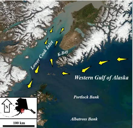
Figure 1.1 Labeled satellite image of Cook Inlet and Western Gulf of AK (NASA).Yellow arrows indicate general current circulation from Gulf of Alaska into lower Cook Inlet along the east side, moving counterclockwise up the inlet before exiting out Shelikof Strait, on the western edge (adapted from Burbank, 1977). This satellite image was taken in May 2014, with

(24)

10 Bottom sediments in lower Cook Inlet are composed of a range of medium- to fine-grained

sands, silts, and clays. There are two primary sources of clay minerals in Cook Inlet: (1) ACC

carrying Copper River clays from the Prince William Sound Region, ~320 km east of Cook Inlet,

and (2) Susitna River in upper Cook Inlet (Hein et al., 1979).

Primary Productivity

The GulfWatch Alaska Program was established by the Exxon Valdez Oil Spill Trustee

Council (EVOSTC) to monitor oceanographic conditions and to provide data to assess impacts of

the Exxon Valdez oil spill in 1989. Part of the 30 year long-term monitoring program has a focused

on lower Cook Inlet oceanographic conditions. The data can be accessed by responders, in the

event of an oil spill in Cook Inlet, to understand historical physical and biological conditions.

Spring and summer samples of the upper water column in Kachemak Bay (“K-Bay” in Fig. 1.1),

a large bay in eastern lower Cook Inlet, and throughout lower Cook Inlet, show high abundances

of diatoms, primarily Chaetoceros spp., and to a lesser extent Pseudo-nitzschia spp., Rhizosolenia

spp.,and Thalassiosira spp. Total cell abundances indicate an annual pattern of a diatom bloom

beginning in late April, peaking in July, and declining to near zero from November to March.

Kachemak Bay, Cook Inlet consistently has the highest phytoplankton abundances (Holderied et

al., 2018).

Sinking Particles

Offshore studies in the northern Pacific and Gulf of Alaska have documented the presence

of NMS (Tsunogai et al., 1982). Laser In Situ Scattering and Transmissonmetry device

(LISST-DEEP) and underwater vision profiler data across the entrance of Cook Inlet have suggested that

some of the particles could be associated with biological production (Turner et al., 2017). Chester

(25)

11 flux quantity and composition reaching the seafloor. Their study explored the seasonality of the

fluxes at three sites with moored sediment traps, finding that Kachemak Bay was highly productive

with efficient particle transport to the seafloor throughout the year.

1.5 Objective of Thesis Research

In a 2016 review of ORMS’ potential for increasing an oil spill’s impact to the benthic

environment, Daly et al. highlighted the urgent need to understand baselines in regions of

hydrocarbon extraction. This thesis research was a preliminary investigation of: (1) the upper

ocean particle flux at four sites in the Kachemak Bay region and (2) the potential for natural surface

water assemblages to incorporate oil in sinking aggregates. The objective of this research was to

test the hypotheses that: (1) there is a high particle flux in Kachemak Bay region with varying

composition over time and space, and (2) that surface waters from lower Cook Inlet would form

ORMS aggregates in the presence of oil in roller-bottles to a similar degree as found in studies

with water from other regions of high primary productivity. The spatiotemporal characteristics of

the baseline flux indicated significant and consistent organic fluxes out of the upper water column

at each site. This study aimed to contribute to the understanding of ORMS as a potential exposure

route that could impact critical habitats with high productivity, like lower Cook Inlet.

1.6 Methods for Thesis Research

Surface-tethered sediment traps were deployed, dovetailing with existing GulfWatch AK

sites, in the Kachemak Bay region to quantify the baseline particle flux. Samples were collected

May through July 2019, June through August 2018 and in January 2019. The quantity and

composition of the fluxes helped inform laboratory oil exposures to simulate a surface oil spill.

Roller-bottles were used in June 2019, with surface water samples, to examine relative oil sorption

(26)

12 contents of roller-bottles suggested significant potential for oil sorption to biological and mineral

constituents in the surface waters of lower Cook Inlet.

1.7 Western Gulf of Alaska Research

In July 2019, particle flux measurements were taken above shallow banks east of Kodiak,

AK in the Gulf of Alaska. Portlock and Albatross Banks (Fig. 1.1), are elevated features

surrounded by isolated deep channels (> 150 m). Both banks have shoals with depths of less than

50 m (Favorite et al., 1975). Recent sampling by Strom et al. (pers. comm., 2019) showed that

there is strong coupling between surface productivity and benthic habits on these banks. The

counterclockwise circulation of the ACC produces nutrient cycling in these areas which results in

high primary productivity above the banks.

With documented connectivity from surface to benthos, there is a high potential particle

flux of organic material. As documented in previous sections, high fluxes, even with high organic

composition, may provide a mechanism for surface oil to reach the seafloor. Due to the distance

from shore ( >24 mi), these regions fall under the pre-authorization zone for Alaska Dispersant

Guidelines. Due to their depth and high connectivity, both physically and chemically dispersed oil

is likely to reach the seafloor much faster at these locations than what is expected in other regions

of the pre-authorized zone. The July 2019 four-day sampling effort at Portlock and Albatross

Banks served as a pilot investigation of the potential for ORMS formation leading to oil transport

(27)

13

2. MATERIALS AND METHODS

2.1 Introduction

Particle flux measurements and laboratory oil incubations were used as a first step in

evaluating the potential formation of ORMS in lower Cook Inlet, AK. A surface-tethered sediment

trap was deployed at four sites in the Kachemak Bay region to explore the spatial and temporal

variation in quantity and composition of sinking particles from surface layers to deeper in the water

column. Laboratory oil incubations were designed to simulate spilled oil conditions relevant to a

very thin (~ 5 μm) surface slick in Cook Inlet waters.

2.2 Study Location

Kachemak Bay is a Subarctic estuary on the eastern side of lower Cook Inlet (Fig. 2.1).

The bay is divided into inner and outer regions by the Homer Spit and is heavily influenced by

glacial inputs that become increasingly greater towards the head of the bay (Holderied et al., 2018).

Deep oceanic waters from the Gulf of Alaska enter along the eastern shore of lower Cook Inlet

and move counterclockwise from the outer to inner bay before exiting around the southwestern

(28)

14

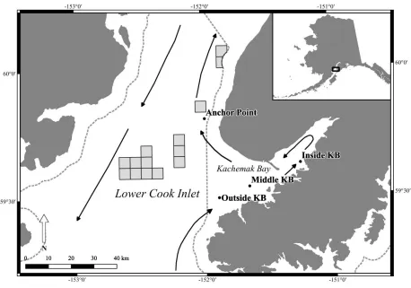
Figure 2.1 Map of lower Cook Inlet showing sites of sediment trap deployments (QGIS). The arrows represent the general circulation pattern (adapted from Burbank, 1977). The Homer Spit divides Kachemak Bay into the inner and outer regions. Water from the Gulf of Alaska moves counterclockwise around Kachemak Bay, along Outside KB, Middle KB, and Inside KB sites, then exits around Homer Spit and towards Anchor Point. The dashed line shows the designation of federally managed Outer Continental Shelf (OCS) waters. Lease blocks receiving bids in Lease Sale 244 are shown in lower Cook Inlet.

Due to seasonal glacial runoff and erosion, the exiting water is fresher and more turbid than

the water entering the bay on the east side (Field and Walker, 2003). The bay is home to a National

Estuarine Research Reserve (NERR) and there is an abundance of long-term data on

oceanographic conditions. In this study, three sampling sites were located along the axis of

Kachemak Bay (two outside Homer Spit, one inside) and are referred to as Outside KB, Middle

KB, and Inside KB (EVOSTC GulfWatch stations KB01, Transect 4 Station 4, and KB09,

(29)

15

location of high deposition off Anchor Point (GulfWatch Transect 3 Station 13) (Fig. 2.1).

Long-term datasets produced by GulfWatch Alaska, and consultation with local professionals on the

Project Advisory Committee (PAC) were essential in providing insight to primary productivity

and oceanographic conditions informing selection of these sites. Following the January 2019

sampling, Inside KB was not visited again, primarily due to its proximity to shore, as oil stranding

would be of higher concern.

A major aspect of the 2018 sampling campaign was the development of a trap deployment

procedure that would work in a high energy estuarine system. Surface tidal currents in the region

can be up to 4 knots. The circulation and energy within the region varies significantly within the

tidal cycle and would likely play a significant role in the fate of pollutants (Burbank, 1977; Hein

et al., 1978).

2.3 Establishing Baseline Particle Flux

Sediment traps are commonly used to directly measure sinking particles. Sediment traps

employ open-top tubes to passively collect sinking particles at a desired depth. Particle fluxes

measured by traps decline with depth and are consistently greater in areas of higher primary

productivity, but there are some limitations to using sediment traps, such as hydrodynamic

(30)

16 surface-tethered sediment trap (Fig. 2.2) was

adapted for deployment in Cook Inlet

conditions. The mixed layer depth from the

middle bay inwards is historically between

10-15 m depending on the season (Doroff &

Holderied, 2018). Therefore, the sediment trap

sampling array and tubes were deployed at 20

m below the surface to collect particles sinking

out of the mixed layer (Lundsgaard et al.,

1999). At the surface, a buoy and a radar

reflector were attached to the top of the trap

assembly. A 2 m shock cord that could stretch

to 3 m was used to mitigate surface wave

energy during deployment. Four submerged

floats were deployed below the shock cord to further reduce vertical movement due to surface

waves (Juul-Pedersen et al., 2006). The main line to which the sampling array was attached

descended to a total depth of 25 m, terminating at a 22 kg weight to maintain vertical alignment

from the surface to the trap. Four 2.4 L tubes were attached to a cross. All tubes had a height to

diameter ratio of 8:1 to limit resuspension of particles (Hargrave and Burns, 1979; Buesseler et al.,

2007). Each tube included a 8 cm deep baffle section consisting of ten 1.5 cm diameter inner tubes

at the top to straighten the flow of particles that were settling into the tube. Each tube was entirely

filled with a 38 PSU solution of artificial seawater (Instant Ocean), measured with a refractometer,

to create a hypersaline density trap for sinking particles (Knap et al., 1997). The artificial seawater Figure 2.2 A schematic of the

(31)

17

was filtered with 0.2 µm membrane filter and stored in a carboy before being poured into tubes

directly before deployment.

The sediment trap was deployed for 1 to 3 h depending on weather and safety

considerations. The start and finish coordinates were recorded for each sediment trap deployment

and used to document the total drift distance over the deployment time. Following collection, the

trap system was brought to the surface using the davit and winch. The tubes were removed and

capped until further processing in the laboratory within 3 h. No preservatives were used between

collection and processing.

In Summer 2018, three of the tubes from each deployment were filtered onto pre-weighed

0.7 um Whatmann GF/F filters (Whatman 1825-047, GE Life Sciences, Marlborough, MA) and

frozen until processed. In 2019 four to eight tubes from each sample were filtered. All filters were

dried for 24 h at 60°C to obtain the dry weight of particles collected (Total Particulate Matter,

TPM). Then, the filters were ignited for 6 h at 500°C and weighed to determine the organic content

(Traiger and Konar, 2017). This measurement was used to estimate the organic portion of the flux

as, referred to as Total Volatile Solids (TVS). Calculations for this process are outlined in Section

2.4.

During each deployment, in situ environmental parameters were measured using a

handheld conductivity, temperature, and depth (CTD) cable-tethered probe (6-series Sonde, YSI

Inc. Yellow Springs, OH). Salinity, temperature and conductivity were recorded in the top 25 m

of the water column next to the sediment trap. Density was calculated (Millero et al., 1980) from

(32)

18 A 5 L Niskin bottle (General Oceanics, Miami, FL) was used to take a grab sample of the

water column at 20 m. 1 L from the water column grab sample was filtered and processed following

the same procedure as sediment trap tube samples. 4.8 L of an additional surface water sample

were used in roller-bottle experiments to study aggregate formation, varying the presence of oil

and additional sediment (The procedure for the roller-bottle experiments is discussed in Section

2.6).

2.4 Particle Flux Calculations

TPM and TVS fluxes were calculated using the equations (Juul-Pedersen et al., 2006). The

solid mass collected on the filter (g) was weighed for a Total Particulate Matter (TPM) (Eq. 1).

The TVS was determined per tube by the change in mass from dry weight to post combustion

weight, which included the ash left on the filter after combustion (Eq. 2) (Traiger and Konar,

2017). Both TPM and TVS masses were normalized into fluxes by dividing by the spatial area of

the tube opening (39.6 cm2_{) and the time of deployment (d) (Eq. 3 and 4).}

(1) 𝑇𝑃𝑀 (𝑔) = 𝐹𝑖𝑙𝑡𝑒𝑟 𝑇𝑎𝑟𝑒𝑑 𝐷𝑟𝑦 𝑊𝑒𝑖𝑔ℎ𝑡 (𝑔) − 𝑆𝑎𝑚𝑝𝑙𝑒 𝐷𝑟𝑦 𝑊𝑒𝑖𝑔ℎ𝑡 𝑎𝑓𝑡𝑒𝑟 60 °𝐶 (𝑔)

(2) 𝑇𝑜𝑡𝑎𝑙 𝑉𝑜𝑙𝑎𝑡𝑖𝑙𝑒 𝑆𝑜𝑙𝑖𝑑𝑠 (𝑔) =

𝐷𝑟𝑦 𝑊𝑒𝑖𝑔ℎ𝑡 (𝑔) − 𝑃𝑜𝑠𝑡 𝐶𝑜𝑚𝑏𝑢𝑠𝑡𝑖𝑜𝑛 𝑊𝑒𝑖𝑔ℎ𝑡 𝑎𝑓𝑡𝑒𝑟 500°𝐶 (𝑔)

(3) 𝑇𝑃𝑀 𝐹𝑙𝑢𝑥 (𝑔 𝑚−2_𝑑−1_{) =} 𝑇𝑃𝑀

𝐴_{𝑇𝑟𝑎𝑝} × 𝑇_{𝐷𝑒𝑝𝑙𝑜𝑦𝑚𝑒𝑛𝑡}

(4) 𝑇𝑉𝑆 𝐹𝑙𝑢𝑥 (𝑔 𝑚−2_𝑑−1_{) =} 𝑇𝑉𝑆

𝐴_{𝑇𝑟𝑎𝑝} × 𝑇_{𝐷𝑒𝑝𝑙𝑜𝑦𝑚𝑒𝑛𝑡}

where 𝐴_{𝑇𝑟𝑎𝑝} (m2) is the sediment trap surface area and 𝑇_{𝐷𝑒𝑝𝑙𝑜𝑦𝑚𝑒𝑛𝑡} is the time (d) the trap

was drifting. The organic portion of each total flux was determined by the Percent Organic,

(33)

19

(5) 𝑃𝑒𝑟𝑐𝑒𝑛𝑡 𝑂𝑟𝑔𝑎𝑛𝑖𝑐 (%) = 𝑇𝑉𝑆 𝑇𝑃𝑀𝑥 100

Mean aggregate particle sinking velocities were estimated (Eq. 6) from the TPM and

concentration at depth (Juul-Pedersen et al., 2006).

(6) 𝑀𝑒𝑎𝑛 𝑠𝑖𝑛𝑘𝑖𝑛𝑔 𝑣𝑒𝑙𝑜𝑐𝑖𝑡𝑦 (𝑚 𝑑−1_{) = 𝑇𝑃𝑀 𝐹𝑙𝑢𝑥 (𝑔 𝑚}−2_𝑑−1_)/𝐶

𝑖𝑛 𝑠𝑖𝑡𝑢(𝑔 𝑚−3)

where the TPM flux is from Eq. 3 and the Cin situ is the concentration of suspended particles

in the Niskin bottle grab sample at the depth of the trap during deployment.

2.5 Roller-Bottle Oil Incubations

Oil incubation experiments were conducted in Summer 2019 to evaluate the potential for

oil sorption and sinking. The studies were conducted at the Kasitsna Bay Laboratory using water

collected during particle flux sampling. ORMS is primarily studied in roller-bottle systems to

investigate formation and sinking of aggregates (Brakstad et al., 2018). Following DWH,

roller-bottles were used in many studies with varying conditions relevant to the GoM and the DWH

response (Passow et al., 2016; Passow et al., 2012; Ziervogel et al., 2012; Passow, 2019). Many

DWH ORMS studies measure the effect of chemical dispersants on flocculation. The roller-bottle

procedure for this research was designed to be relevant for surface oil slick interactions in the days

following a tanker spill (t = 5 d; oil slick = 5 μm; headspace in bottle simulating surface slick rather

than dispersed droplets). Specific mechanisms of aggregate formation, biodegradation of oil,

transport, and water column aggregate fragmentation were not addressed in this study.

2.6 Roller-Bottle Procedure

Three identical roller-bottle incubation experiments were conducted. Surface water was

collected in a 5 gallon carboy, rinsed with surface water three times, off the side of the vessel

(34)

20

experiment, 1 L of surface water was filtered using GF/F for surface water characterization of

TPM and TVS. Eight 0.95 L (32 oz.) glass bottles (wide-mouth, Uline; Chicago, IL) each received

800 mL of surface water. The inside of each glass bottle’s plastic lid was lined with Teflon to limit

oil sorption.

Table 2.1 Experimental set-up for roller-bottle incubations

Experimental Condition Seawater Volume (mL) ANS Oil (μl) Sediment (mg)

W 800 - -

W + S 800 - 160

W + O 800 80 -

W + S + O 800 80 160

Four bottles each received 80 μl of ANS crude oil from a positive displacement pipette

(Prince et al., 2016). While oil property characterization was not conducted in this study, ANS

crude produced in 2015 had an API gravity between 17° and 31° depending on temperature and

mass lost from evaporation (water has an API of 10°) (Hollebone, 2015). The resulting nominal

oil concentration was 80 μl oil/ 800 mL seawater or 0.01% oil by volume (100 ppm), but is more

appropriately characterized by a surface sheen thickness of ~5 μm. This thickness was estimated

(Eq. 7) by measuring the surface area of the slick inside the bottle when it was horizontal in rolling

position and assuming all oil spread over this area evenly.

(7) 𝑂𝑖𝑙 𝑡ℎ𝑖𝑐𝑘𝑛𝑒𝑠𝑠 (𝜇𝑚) = 𝑉𝑜𝑙𝑢𝑚𝑒 𝑜𝑓 𝑜𝑖𝑙 (𝑚𝑚

3₎

𝐿𝑒𝑛𝑔𝑡ℎ 𝑜𝑓 𝑜𝑖𝑙 (𝑚𝑚) 𝑥 𝑤𝑖𝑑𝑡ℎ 𝑜𝑓 𝑜𝑖𝑙 (𝑚𝑚)𝑥

(35)

21

where volume is 80 mm3_{, length is 80 mm, and the width is 95 mm (determined by}

manually measuring the dimensions of the bottle), resulting in a nominal thickness of ~5.2 μm.

This concentration in the jar created a sheen that would be defined as “metallic” and

considered unrecoverable by mechanical response methods (NOAA, 2016). Sediment from

Nikiski, AK (middle Cook Inlet), was added to four of the bottles at a nominal concentration of

200 mg/L, which is a realistic concentration of suspended matter found in the middle and upper

inlet (Table 2.1) (Hein et al., 1979). The sediment was collected and supplied by the Cook Inlet

Regional Citizens Advisory Council (CIRCAC). The sediment was air dried and a portion of the

same sample used in OMA studies by Khelifa et al. (2008). The sediment sample used was

characterized by Khelifa et al. in 2008 to be 49% fine content (weight of grains less than 5.3 μm

in diameter), with a density of 2.58 ± 0.11 g/mL and an organic matter content of 3.3 ± 0.1%. The

experimental conditions in the bottles were: whole surface water only (W), surface water +

sediment (W+S), surface water + oil (W+O), and surface water + sediment + oil (W+S+O) (Fig.

2.3).

The bottles were then placed on the rolling apparatus (Wheaton Roller Bottle Apparatus,

Dual Deck W348924-A, Millville, NJ) at a speed of 4 rpm under constant light (two 40W bulbs)

(36)

22

temperature throughout Kachemak Bay (Holderied et al., 2018). The ~200 mL headspace allowed

for surface mixing, unlike procedures previously used to simulate non-turbulent water column

ORMS formation (Ziervogel et al., 2014).

2.7 Roller-Bottle Data Collection

Qualitative observations of when visible aggregates began to form were recorded during

the incubation. After 120 h, the bottles were removed from the apparatus and set upright (as

pictured in Fig. 2.3) on the laboratory bench to allow contents to settle. Qualitative visual estimates

of relative aggregate abundance, size, and settling rates were recorded for each treatment condition

as bottles were removed from the rolling apparatus.

After 1-3 h of settling, the surface oil sheen was manually removed with a sorbent pad

(piece of 15 x 19” heavy hydrophobic/oleophilic marine oil sorbent pad). Five aggregates were

extracted from one bottle of W and W+S (10 total aggregates from oil negative treatments), and

five aggregates were extracted from both replicate W+O and W+S+O bottles (20 total aggregates

from oil positive treatments). The aggregates (W and W+O) and settled sediment ridden material

(in the case of W+S and W+S+O) were extracted using a 3 mL plastic transfer pipette that had

been trimmed to have a blunt tip. Aggregates were analyzed using 10x ocular and 10x objective

lenses with a Nikon Eclipse 80i microscope with fluorescence powered by an X-Cite series 120

UV lamp (MVI; Avon, MA). The aggregates were pipetted onto glass slides and were immediately

covered with a glass slip and placed under the microscope. Fluorescent light was used to

distinguish the oil droplets, which fluoresce, from non-fluorescing detritus and minerals in the

aggregates (Stoffyn-Egli and Lee 2002; Loh et al., 2014). Photomicrographs were taken of

aggregates with and without fluorescence for image analysis with the program ImageJ (Rasband,

(37)

23

of oil negative control aggregates were taken to determine the level of background fluorescence.

All photomicrographs were taken with an iPhone 7 using a LabCam Microscope Adapter and a

10x ocular lens (total magnification 100x).

Following microscopy, the contents of the bottles were filtered on GF/F to determine TPM

and TVS following the same processing procedure as was used for the sediment trap tubes (Section

2.4; Eq. 1 and Eq. 2). Contents from the upper portions of the bottle were extracted with a 50 mL

plastic syringe and weighed before filtration. Contents remaining in the lower portion of the bottle

were poured directly into another jar to weigh before filtering. The masses were recorded instead

of approximating volumes with a beaker.

2.8 Statistical Analysis

Particle Flux

Significance tests were performed with JMP14 software (SAS Institute Inc.; Cary, NC) to

examine the variation of the particle flux spatially and temporally. Due to a processing mistake

during the combustion of filters, some of the organic content data points from Summer 2018 were

lost. For January 2019 and May-July 2019, all tubes were successfully processed.

Interannual fluxes were compared between the two sites with the highest number of

samples (Middle KB and Outside KB). Due to significant differences in flux quantity and

composition between years, sites in 2018 and 2019 were not pooled together. Due to the relatively

low sample sizes (n= 3-8), one-way ANOVAs were used instead of nonparametric tests for

significance (Ramsey, pers. comm., 2019), except in cases of comparing data with high variances,

then a Kruskall Wallis test was used, and indicated in reporting significance. Student’s t-tests were

(38)

24

Roller-Bottles

TPM and TVS concentrations were split into two parts of each bottle, upper and lower,

representing the upper 600 ± 15 mL and lower 130 to 200 mL depending on how much water

volume was adsorbed by the sorbent while manually removing the oil slick. Student’s t-tests were

used for all two-factor comparisons (α=0.05). Statistical analyses were performed using JMP 14

software.

Photomicrographs were used to make estimates of oil content in aggregates. Because

aggregates were not randomly selected within each bottle and they often fragmented while making

slides, statistical analyses were not possible with resulting data. Clear photos of aggregates were

made into binary images using ImageJ. These photomicrographs were representative of each

experimental condition and were used to quantify the potential amount of oil associated within the

extracted ORMS. Oil estimates obtained from the fluorescent photomicrographs were compared

to total aggregate size. The resulting value was a two dimensional ratio of oil to aggregate surface

area and referred to as “percent oil cover”.

The volume of oil that was incorporated in ORMS was estimated using Feret’s diameters

(calculated maximum diameter of non-spherical objects) assumed of fluorescing oil droplets in

five W+O aggregates, assuming droplets in the aggregates were spherical. Images of five W+O

aggregates were used to estimate total content. These images were chosen because they were

within one standard deviation of the percent oil cover and considered representative aggregates for

further estimates, rather than estimating volume from outlying aggregates with high fluorescence

from a single large droplet. Fluorescing droplets with Feret diameters of less than 10 μm were not

included in estimates of volume. This diameter limit was determined as a reasonable lower limit

(39)

25 included the 10 largest droplet volumes calculated from each image, which represented on average

78% of the total volume of fluorescing droplets.

The specific procedure for volume analysis in ImageJ may be found in Appendix A. Others

have attempted oil quantification from two-dimensional pictures of aggregates (Payne et al., 1987,

2003; Lee and Stoffyn-Egli, 2002; Khelifa et al., 2002) and found that oil volume estimates may

not be appropriate when aggregates are large or have complex shapes (Khelifa et al., 2007; Loh et

al., 2014). If there is enough oil in aggregates, GC-FID and or GC-MS could be applied to measure

oil concentration (Bragg and Owens, 1994; Bragg and Yang, 1995; Khelifa et al., 2008).

2.9 Western Gulf of Alaska Sampling

(40)

26 During a July 2019 field sampling event at Portlock and Albatross Banks (Gulf of AK), the

same methods (Section 2.2) were used to measure and document particle flux and composition.

Sediment traps with four tubes were deployed for 4 to 5 h each a total of three times at three sites

on each bank (Fig. 2.4). The trap was lowered to 40 and 50 m below the surface on Portlock and

Albatross Banks, respectively, to give better insight to what is reaching the seafloor (rather than

what is assumed to be falling out of the mixed layer, as in Kachemak Bay at 20 m). Total water

depths ranged from 60 to 80 m on Portlock Bank and 75 to 80 m at Albatross Bank. CTD (SBE

19plus V2 SeaCAT Profiler, Sea-Bird Scientific; Bellevue, WA) casts were recorded to the bottom

of the water column at each site within 1 h of trap deployment. Additional water samples (at the

surface and at the depth of trap) were taken following the same procedure as described in Section

2.3.

All samples were filtered onboard within 1 h of retrieval and filters were frozen until

processing for TPM and TVS values upon return to Kasitsna Bay. Statistical analyses of fluxes

and sinking velocities were conducted in the same manner as described for the Kachemak Bay

(41)

27

3. RESULTS AND DISCUSSION

3.1 Water Column Characterization

Throughout the 2018 and 2019 sampling seasons, water column stratification was different

between sites. Stratification increased from Outside KB to Inside KB. Depths at Outside KB,

Middle KB, and Inside KB were 70 m, 87 m, and 63 m, respectively.

From May through July, vertical density profiles (Fig. 3.1) showed a distinguishable mixed

layer had formed in the upper 6 m of the water column at Middle KB. Inside KB (only measured

with the YSI two times in July 2018) showed stratification in the upper 10 m, likely due to its

proximity to significant freshwater input from the Grewingk glacial lake and watershed.

Anchor Point was unstratified, even with freshwater entering the area from the Anchor

River ~ 7 km east of the site. The completely mixed water column indicated strong connectivity

from surface to benthos. Anchor Point is much shallower, with a bottom depth of ~30 m, than at

sites along the KB axis. The density profiles and physical oceanographic conditions of the area

make Anchor Point distinct from the natural gradient of the other three sites along the axis of KB.

There are indications of convergence between two water masses in the area as documented by

(42)

28

(43)

29 Quarterly CTD casts along the KB axis and a transect near Anchor Point conducted by the

GulfWatch program document similar mixed layer depths interannually (Holderied et al., 2018).

Historical data show a uniform water column enters Cook Inlet from the southeast and remains

unstratified until reaching Middle KB. As the counterclockwise currents move along the bay,

increased terrestrial freshwater inputs off of the southeast side of KB introduce less dense

freshwater creating a stratified water column (Holderied et al., 2018). The same signals of

increasing stratification from freshwater as summer progressed were measured on site when

sediment traps were deployed during 2018 and 2019.

The GulfWatch data was useful in describing the water column characteristics for sampling

events when the YSI was not used (e.g., January 2019) [N.B., GulfWatch data for January 2019

were not available when this thesis was written]. GulfWatch data of the axis in January 2017 and

2018 show slightly less saline (a proxy for density in the system) surface waters along the bay (31

PSU at surface and 32 at depths > 50 m). In 2017 and 2018, the water column was well mixed

along the outer axis in March with increasing freshwater stratification from Homer Spit inward

beginning in April. Past CTD casts from the Anchor Point transect also confirm what was observed

on sampling days in 2019. At Anchor Point, the water column was completely mixed from surface

to the seafloor in February and April, 2016. In August 2016, there was slight stratification in the

upper 5 m of the water column at Anchor Point, but not as extreme as Inside KB. Oceanographic

data is not collected as regularly along the Anchor Point transect due to longer transit times,

rougher seas, and harsher weather in the lower inlet. Overall, the density profiles recorded on

sampling days were similar to previous years’ profiles suggesting the water column characteristics

(44)

30

3.2 Flux Summary

TPM fluxes were slightly higher in 2018 than 2019. TVS fluxes were similar over both

seasons. During 2019, efforts were focused on characterizing the flux at Outside KB, Middle KB,

and Anchor Point. Anchor Point became a location of interest after one exploratory sample in 2018

showed considerably higher fluxes. A decision was made by the project team to substitute Anchor

Point for Inside KB in the 2019 sampling plan. As a result, interannual comparisons were only

possible for Middle KB and Outside KB (Table 3.1).

Table 3.1 Sample replicates from all events from June 2018 to July 2019. [N.B., Fewer 2018 samples were successfully processed for loss on ignition due to data processing issues].

Site

Total Deployments

Total Replicates Processed for TPM

Total Replicates Processed for TVS

2018 2019 2018 2019 2018 2019

Anchor Point 1 4 3 24 3 24

Inside KB 5 1* 15 4 8 4

Middle KB 5 5* 15 28 11 28

Outside KB 5 4 12 20 10 20

Gulf of AK - 6 - 24 - 24

*Including one deployment on January 24, 2019

There were significant differences in total flux and variances between Anchor Point and

the KB sites (Fig. 3.2). The TVS portion of the flux was consistent from site to site and from 2018

(45)

31

Figure 3.2 Bar graph showing TPM, TVS, and with standard error bars. Data omitted from graph: January 2019 Samples and Anchor Point 2018 (n=1).

Table 3.2 Summary table of TPM and TVS fluxes (excluding January 2019 and Anchor Point 2018 samples)

Site TPM Flux 2018 (g m-2_d-1₎

TVS Flux 2018 (g m-2_d-1₎

TPM Flux 2019 (g m-2_d-1₎

TVS Flux 2019 (g m-2_d-1₎

Anchor Point - - 250.7 ± 185.5 36.4 ± 13.9

Inner KB 150.9 ± 40.3 41.4 ± 12.8 - -

(46)

32

Table 3.3 Mean concentrations of suspended matter at the depth of the trap by site (excluding January 2019 and Anchor Point 2018)

Seasonal comparisons of means (Table 3.2) showed differences between years. At Middle

KB, TPM fluxes were not significantly different (NSD) from 2018 to 2019 (p-value = 0.1015).

The last sample of 2018 (August) and the first sample of 2019 (May) were likely driving these

results. When a Student’s t-test was run without those two sampling events, the 2018 fluxes were

significantly higher than in 2019 (161 ± 32 g m-2 d-1 and 83 ± 34 g m-2 d-1 in 2018 and 2019,

respectively) (p-value < 0.0001). The suspended matter TPM and TVS concentrations at the depth

of the trap were similar across sites (Table 3.3).

At Middle KB, TVS had nearly identical means from 2018 to 2019 (p-value = 0.9900).

However, because the TPM decreased in 2019, the percent of the flux that was attributed to

organics (30 ± 7% and 37 ± 8% in 2018 and 2019, respectively) increased significantly (p-value =

0.0195).

Variation in fluxes between years at Outside KB was similar to what was observed at

Middle KB. The TPM fluxes in 2018 were significantly higher (Student’s t-test p-value = 0.0093)

with means of 132 ± 32 g m-2 d-1 and 87 ± 51 g m-2 d-1 in 2018 and 2019, respectively. Distributions

of data at Outside KB were fairly uniform and there were no divergent samples, like 5/11/2019

and 8/3/2018, in Middle KB.

Site Suspended TPM _{at 20 m (g m}-3₎

Suspended TVS at 20 m (g m-3₎

Anchor Point 27.3 ± 9.7 9.5 ± 2.1

Inner KB 29.3 ± 1.3 8.2 ± 1.3

Middle KB 21.8 ± 6.5 7.8 ± 1.9

(47)

33

The TVS fluxes from 2018 to 2019 at Outside KB had NSD (t-test p-value =0.1084). At

Outside KB, TVS fluxes did slightly decrease, but the TVS fluxes were still relatively close from

2018 to 2019 with means of 38 ± 12 g m-2 d-1 and 30 ± 14 g m-2 d-1, respectively. The organic

percentage of the flux significantly increased from 2018 to 2019 (Student’s t-test p-value = 0.0376)

with means of 28 ± 5% and 38 ± 11% organics.

A potential explanation for the significant decrease in the TPM flux at Outside KB and

Middle KB between 2018 and 2019 was rainfall in the region. The suspended sediment load

entering southeastern Cook Inlet is comprised of clay minerals originating in the Copper River,

Northern Gulf of Alaska (NGoA) (Fig. 1.1) (Hein et al., 1979; Feely et al., 1982). The Copper

River discharge (measuring outflow of a 24,030 sq. mi. drainage area at Million Dollar Bridge in

Cordova Valdez Consensus Area) in April 2018 was 30,950 cubic feet per second (cfs) at the same

site, the April 2019 was over four times lower at 7,357 cfs. The discharge difference was less

significant in May and June, with flow decreases of 6,000 cfs in May and a 1,500 cfs increase in

June, from 2018 to 2019 (Fig. 3.3) (USGS, 2019). Higher spring flows and sediment loads in 2018

could be responsible for higher inorganic particles loads in lower Cook Inlet, especially at the

Outside KB and Middle KB sites. Furthermore, the KB region was notably dry in Summer 2019.

The Homer, AK airport rain gauge only recorded 0.22 inches of rain in May and June 2019,

compared to 3.97 inches of rain in the same months of 2018. This highlights the role of terrestrial

(48)

34

Figure 3.3 Mean Copper River discharge in 2018 to 2019 at the Million Dollar Bridge USGS station (USGS, 2019)

3.3 Spatiotemporal Analysis of Fluxes

2018 fluxes were NSD from site to site (ANOVA p-value = 0.5374) (151 ± 40, 136 ± 59,

and 132 ± 32 g m-2 d-1 at Inside KB, Middle KB, and Outside KB, respectively). Comparisons for

each pair using Student’s t-tests also showed that the three 2018 sites were NSD from each other.

While there were NSD, an ordered differences report indicated a gradient in TPM flux increasing

(49)

35

An analysis of TVS also showed NSD in composition between the KB sites (ANOVA

p-value = 0.7216). Student’s t-test comparisons between each site with an ordered differences report

also showed NSD in TVS flux.

In an analysis of 2019 samples, Anchor Point clearly had a significantly higher flux

(Kruskal Wallis p-value of < 0.0001). Outside KB and Middle KB were not significantly different

in 2019 TPM fluxes (p-value = 0.6274). The mean TPM fluxes were 251 ± 186 g m-2 d-1, 104 ± 57

g m-2 d-1, and 87 ± 51 g m-2 d-1 at Anchor Point, Middle KB, and Outside KB, respectively.

There were no significant differences in TVS between sites in either year, including Anchor

Point (Kruskall Wallis, p-value = 0.1809). The 2019 TVS means were 36 ± 14 g m-2 d-1,

36 ± 17 g m-2 d-1, and 30 ± 14 g m-2 d-1 at Anchor Point, Middle KB, and Outside KB, respectively.

There were slightly higher organics sinking at Anchor Point, but these were NSD. Although there

was a lower percent of organics at Anchor Point (20%, compared to 37% TVS at both Middle KB

and Outside KB), the mass of organics remained high compared to other sites suggesting surface

oil sorption to biological components could be as relevant in this area and potentially enhanced by

the high quantity of inorganics sinking.

There was no trend in TPM flux within each season. In May 2019, one sampling event at

Middle KB had significantly higher TPM and TVS fluxes than the three later visits to that site over

June and July. May 2019 samples from Outside KB had higher variation in TPM and TVS than

the rest of the summer, but there was NSD in either flux from May to July 2019. While sample

sizes within months were relatively low, there was no indication of significant variation driven by

time within a sampling season, which aligns with GulfWatch plankton abundance data for KB.

POTENTIAL ROLE OF MARINE SNOW IN THE FATE OF SPILLED OIL IN COOK INLET, ALASKA

University of New Hampshire Scholars' Repository

University of New Hampshire Scholars' Repository

POTENTIAL ROLE OF MARINE SNOW IN THE FATE OF SPILLED

POTENTIAL ROLE OF MARINE SNOW IN THE FATE OF SPILLED

OIL IN COOK INLET, ALASKA

OIL IN COOK INLET, ALASKA

POTENTIAL ROLE OF MARINE SNOW IN THE FATE OF

SPILLED OIL IN COOK INLET, ALASKA

ACKNOWLEDGEMENTS

TABLE OF CONTENTS

LIST OF TABLES

LIST OF FIGURES

LIST OF ACRONYMS

ABSTRACT

1. INTRODUCTION

2. MATERIALS AND METHODS

3. RESULTS AND DISCUSSION