Rarity and commonness in New Zealand ferns

(1)

Lincoln University Digital Dissertation

Copyright Statement

The

digital

copy

of

this

dissertation

is

protected

by

the

Copyright

Act

1994

(New

Zealand).

This

dissertation

may

be

consulted

by

you,

provided

you

comply

with

the

provisions

of

the

Act

and

the

following

conditions

of

use:



_you

_will

_use

_the

_copy

_only

_for

_the

_purposes

_of

_research

_or

_private

_study



you

will

recognise

the

author's

right

to

be

identified

as

the

author

of

the

dissertation

and

due

acknowledgement

will

be

made

to

the

author

where

appropriate



you

will

obtain

the

author's

permission

before

publishing

any

material

from

the

dissertation.

(2)

Rarity and Commonness of

New Zealand Ferns

A Dissertation

submitted in partial fulfilment

of the requirements for the Degree of

Bachelor of Science, Honours, in Conservation and Ecology

at

Lincoln University

by

Catherine Frances Mountier

(3)

Abstract of a Dissertation submitted in partial fulfilment of the

requirements for the Degree of Bachelor of Science, Honours, in Conservation

and Ecology

Abstract

Rarity and Commonness of

New Zealand Ferns

by

Catherine Frances Mountier

A macroecological approach was used to look for patterns in, and correlates of, rarity and

commonness in the New Zealand fern flora, which is comprised of 250 species. Herbarium records and expert knowledge were used to map fern species distributions from which range sizes were calculated, and used as a measure of rarity and commonness. Fern species frequency distributions showed a pattern of many small and fewer large range sizes, with bimodal peaks at very small and medium range sizes. Latitudinal differences in range sizes showed evidence of a geometric constraint and the mid-domain effect, and did not directly support Rapoport’s Rule which suggests larger range sizes at higher latitudes and vice versa. Trait data for each fern species, including morphological characteristics, were compiled from the literature, as were habitat preferences, elevational range, and biostatus,. Both univariate and multivariate linear mixed models were used to determine relationships between species traits and range sizes for 211 fern species for which data were available. Habitat specialists had smaller range sizes than generalists, and species occurring in forest and/or montane environments had larger range sizes than those that did not, as did epiphytic species. The variation in range size explained by phylogeny (taxonomic family and genus) was lower than that explained by traits. Patterns of rarity and commonness differed markedly between

indigenous and introduced species. This study provides new knowledge of patterns in the diversity of the New Zealand fern flora.

(4)

Keywords: Ferns, rarity, range size, linear mixed models, Rapoport’s Rule, mid-domain effect, endemism, biostatus, New Zealand.

Acknowledgements

Many thanks to my supervisor Hannah Buckley, and Brad Case for the GIS component. Thanks to Leon Perrie and Patrick Brownsey at Te Papa for checking and correcting fern species distributions, and advice on numerous details of this study. The herbaria at Te Papa, the Auckland War Memorial Museum and the Allan Herbarium at Landcare Research provided herbarium records for fern species which form the basis of the spatial data in this study. Marian Dassonneville and Anais Tieche

extracted and entered some of the fern trait data. Lincoln University and the Freemasons for

financially supported my studies this year. Thanks to my fellow students for camaraderie and mutual support, and special thanks to Phil Holland and Jane Mountier for helping me achieve this goal.

(5)

List of Tables

Table 1.1 A typology of rare species based on three characteristics (after Rabinowitz 1981). ... 2 Table 2.1 Fern traits used in analyses, variable types, levels or units of variables, and

explanations...19 Table 2.2 A priori hypotheses: predictions and rationale for variables used in analyses. ...22 Table 2.3 The three multivariate model sets used, including model codes, model names, and the

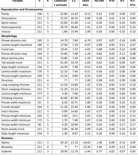
variables included in each model. ...26 Table 3.1 Pearson correlation coefficients for correlations among four different measures of range size. ...30 Table 3.2 Linear mixed effects model coefficient values and standard errors (S.E.) and AICc model

comparison statistics showing the relationships between fern range sizes and species’ traits. Delta AICc and AICc weights were calculated in comparison to a null, intercept-only model, therefore negative numbers mean that there was more support for the tested variable than for the null model, positive numbers mean there was less support. Italicised variable rows are those that were greater than or equal to 2 AICc points less than the null model, indicating support for the importance of the variable in explaining range size. Sample sizes (n), the number of model parameters (K), and the variance explained by the fixed effects alone (R²m), the fixed and random effects combined (R²c), and the random effects alone (R²c - R²m) are given. ...36 Table 3.3 Multivariate model set 1, n=211. Linear mixed effects model AICc model comparison

statistics showing the relationships between fern range sizes and groups of species’ traits. Delta AICc and AICc weights were calculated in comparison to all other models in the set and a null, intercept-only model. Models in italics were identified as the best model set because they were more than two AICc points lower than the next best model. The number of model parameters (K), the log likelihood of the model fitting the data better than the other models (LL), the variance explained by the fixed effects alone (R2m) and the fixed and random effects combined (R2c) are given. Model set codes are explained in Table 2.3 in methods section. ...47 Table 3.4 Multivariate model set 2, n=182, includes some morphological variables not included in

the first set of models. Linear mixed effects model AICc model comparison statistics showing the relationships between fern range sizes and groups of species’ traits. Delta AICc and AICc weights were calculated in comparison to all other models in the set and a null, intercept-only model. The number of model parameters (K), the log likelihood of the model fitting the data better than the other models (LL), and the variance explained by the fixed effects alone (R2m) and the fixed and random effects combined (R2c) are given. Model set codes are explained in Table 2.3 in methods section. ...50 Table 3.5 Multivariate model set 3 uses the smallest data set, n=41, and is comprised of

introduced species only, including casual species which are excluded from the other models sets. Linear mixed effects model AICc model comparison statistics showing the relationships between fern range sizes and species’ traits. Delta AICc and AICc weights were calculated in comparison to all other models in the set including a full model, and a null, intercept-only model. The number of model parameters (K), the log likelihood of the model fitting the data better than the other models (LL), and the variance explained by the fixed effects alone (R2m) and the fixed and random effects combined (R2c) are given. Model set codes are explained in Table 2.3 in methods section. ...50 Table 3.6 Predictions from hypotheses and model results. ⃝ = No relationship with range size, √

= Prediction confirmed, X = Opposite pattern shown. ...52

(8)

List of Figures

Figure 1.1 Abundances of fish species in the Wabash River (Pyron 2010). ... 3 Figure 3.1 Range sizes of all New Zealand fern species, calculated using (a) ecological districts, (b)

ecological regions, (c) polygons, (d) latitudinal extent. ...29 Figure 3.2 Scatterplots showing the correlations among the four different measures of range

size. ...30 Figure 3.3 Species range size distributions for three measures of range size: (a) ecological districts

(b) ecological regions (c) polygons. ...31 Figure 3.4 Species frequency distributions of (a) latitudinal extent (b) latitudinal maximum (c)

latitudinal minimum and (d) latitudinal midpoint. ...32 Figure 3.5 Rapoport’s Rule: scatterplots of species range sizes plotted against (a) latitudinal

minimum, (b) maximum, (c) midpoint and (d) extent. ...33 Figure 3.6 Number of species of introduced, native and endemic species shown in four range size

classes. The range size classes do not have equal ranges, but each represents a similar number of species (~60). In this graph natives and endemics are mutually exclusive. Introduced (including casuals) n = 46, native n = 106 , endemic n = 88. ...34 Figure 3.7 Range sizes of endemic, native and introduced species, plotted against species in

ranked order from smallest to largest. Introduced (including casuals) n = 46, native n = 106 , endemic n = 88. ...34 Figure 3.8 Range size and frond size, n=193. The three species with the largest fronds were the

tree ferns: Cyathea dealbata, Ptsisana salicina and Cyathea medullaris. ...38 Figure 3.9 Range size and maximum lamina length, n=186. ...38 Figure 3.10 Range size by minimum number of pinnae divisions, n=169. ...39 Figure 3.11 Range size by biostatus, n=211. (a) Introduced (n=19) and indigenous species (n=192).

(b) Non-endemics, meaning natives and introduced (n=123) and endemics (n=88). The horizontal bar shows the median value and the box encompasses the

interquartile range. The whiskers extend to the most extreme point which is no more than 1.5 times the interquartile range from the box (R Core Team 2013). ...40 Figure 3.12 Biostatus and range size n=211. Natives n=104, introduced n=19, endemics=88. In this

graph natives and endemics are mutually exclusive. The horizontal bar shows the median value and the box encompasses the interquartile range. The whiskers extend to the most extreme point which is no more than 1.5 times the interquartile range from the box (R Core Team 2013). ...40 Figure 3.13 Years since naturalisation and range size, n=41. The species with largest range sizes

are Selaginella kraussiana and Equisetum arvense, followed by Dryopteris filix-mas and Adiantum raddianum. The five species which have been naturalised the longest are Pteris cretica, Osmunda regalis,Cystopteris fragilis, Polystichum proliferum, and Polystichum setiferum. ...41 Figure 3.14 Number of global regions and range size n=211...42 Figure 3.15 Altitudinal zones which show a positive relationship with range size n=211. Lowland,

Montane, Subalpine. Width of boxplots is proportional to number of species in that category. The horizontal bar shows the median value and the box encompasses the interquartile range. The whiskers extend to the most extreme point which is no more than 1.5 times the interquartile range from the box (R Core Team 2013). ...43 Figure 3.16 Range sizes of number altitudinal zones in which species occur, from one to five,

n=211. No species occurred in all five altitudinal zones...44 Figure 3.17 Habitat generalists and specialists n=211. Width of boxes is proportional to n in that

category. Generalists n=188, Specialists n=23. The horizontal bar shows the median value and the box encompasses the interquartile range. The whiskers extend to the most extreme point which is no more than 1.5 times the interquartile range from the box (R Core Team 2013). ...44

(9)

Figure 3.18 Specialist types n=211. Generalists n=188 , coastal n=11 , base-rich n=2 , aquatic n=4 , thermal n=11 , hot rock n=4 , gumland n=1. The horizontal bar shows the median value and the box encompasses the interquartile range. The whiskers extend to the most extreme point which is no more than 1.5 times the interquartile range from the box (R Core Team 2013). ...45 Figure 3.19 (a) Forest habitat n=127, not forest n=84 (b) Epiphytic n=63, not epiphytic n=148.

Width of boxes is proportional to n for that category. The horizontal bar shows the median value and the box encompasses the interquartile range. The whiskers extend to the most extreme point which is no more than 1.5 times the interquartile range from the box (R Core Team 2013). ...46 Figure 3.20 Model average predicted square root transformed range size values for species n=211

which occur in dry habitats are larger than for species in habitats which are not dry, and the same is shown for species which occur in open habitat types, as generated from model set 1 (Table 3.3). Error bars indicate one standard error. ...48 Figure 3.21 Model average predicted square root transformed range size values for number of

altitudinal zones in which a species occurs, n=211. Five zones were represented in the data, but no species occupied all five. The dotted lines indicate one standard error. ...48 Figure 3.22 Predicted square root range sizes for species in three categories of rhizome/trunk

types. n = 211 and error bars are standard errors. ...49 Figure 3.23 Model averaged predicted square root range sizes for number of years since species

were naturalised. Dotted lines show standard errors, n=41. ...51 Figure 3.24 Model averaged predicted square root range sizes for number of global regions in

which a species is known to occur. The possible number of regions is 7, but no

species scored higher than 5. Dotted lines show standard errors, n=41. ...51

(10)

Chapter 1 Introduction

“Who can explain why one species ranges widely and is very numerous, and why another allied species has a narrow range and is rare?” Charles Darwin (1859)

1.1 Background

Many ecological studies have looked for drivers of variation in distributions of species, but much is still unknown. Patterns of species richness, and patterns of rarity and commonness have been studied using a wide range of plant and animal taxa; however, the causes of these patterns are still under debate (Fiedler & Ahouse 1992; Gaston 1994). This study focuses on patterns of rarity and commonness using New Zealand ferns and fern allies (monilophytes and lycophytes) as the study group. From this point on I will refer to them simply as ferns, unless referring to lycophytes specifically. New Zealand ferns are an ideal group for studying distributions because with approximately 250 species it is small enough to be manageable, but also exhibits variability in habitat preferences, life forms and distribution patterns. New Zealand ferns are well known taxonomically and botanically (Brownsey & Smith-Dodsworth 2000; Breitweiser et al. 2009), but little is known about their large scale ecological patterns. In this study I use geographic range size as a measure of relative rarity or commonness and investigate the relationships between range size and various ecological traits.

Rare species tend to be more at risk, and are therefore of conservation concern, but here I focus on the ecological, biological, and evolutionary causes of rarity without particular reference to conservation status or extinction risk. Anthropogenic impacts, especially in recent decades, are undoubtedly contributing to rarity more than ever before, but the focus of this study is the inherent ecological and biological causes of rarity and commonness, rather than those imposed by humans.

All biological communities have some rare species and some which are common, typically more of the former than the latter (Gaston 1996). What are the forces at play? And how do they interact? What creates this pattern? Is it competition, adaptation or dispersal abilities? Or is it ecological or evolutionary characteristics and constraints? Rarity and commonness occur on a continuum, separated by arbitrary delineations. Similarly, causes of rarity depend on how rarity has been defined and what scales, spatial and temporal, are considered (Rabinowitz 1981; Gaston 1994). There is little evidence to support the idea of a defined set of traits that cause rarity, and actually the

(11)

causes are heterogeneous and context-dependent (Rabinowitz 1981), and also scale dependent (Gaston 1994). Gaston (1994) maintains that it is likely that the processes that constrain the abundance and range sizes of rare species are the same processes that limit common species, not something specific to rarity. The variety of taxa studied and the huge variation in their life forms, add to the difficulties in generalising about causes of rarity and commonness.

1.2 What is Rarity?

Taxa can be rare in differing ways, which can create much confusion if this is not made explicit. In a biological context rare species are recognised as those with low abundance and/or low range-size (Gaston 1994). What is meant by “low” depends on the context, and how abundance and range-size are determined also varies.

Deborah Rabinowitz classified seven different types of rarity (Rabinowitz 1981). She created a theoretical framework using a 2 x 2 x 2 matrix and three characteristics: geographic range, habitat specificity, and local population size. A species is classified as having either a large or small geographic range; a wide or narrow habitat specificity; and a large or small local population size. Together this creates eight categories, of which only one defines commonness, and seven define different types of rarity (Table 1.1).

Table 1.1 A typology of rare species based on three characteristics (after Rabinowitz 1981).

Geographic Range Large Small

Habitat Specificity Wide Narrow Wide Narrow

Local Population Size Large, dominant somewhere Locally abundant over a large range in several habitats

Common

Locally abundant over a large range in a specific habitat Predictable Locally abundant in several habitats but restricted geographically Unlikely Locally abundant in a specific habitat but restricted geographically Endemics Small, non-dominant Constantly sparse over a large range and in several habitats

Sparse

Constantly sparse in a specific habitat but over a large range Constantly sparse and geographically restricted in several habitats Non-existent? Constantly sparse and geographically restricted in a specific habitat

Rabinowitz’s classification system, which has been widely used since 1981, has made explicit the different types of rarity and given a clear structure for subsequent studies of rarity.

(12)

Nevertheless, this classification system does not directly address causes of rarity (Fiedler & Ahouse 1992). Rarity is common, commonness is rare (Fiedler & Ahouse 1992). This can be seen in

histograms of either abundances or range sizes of species in a community which are typically right skewed and concave, (e.g. Figure 1.1) indicating a few species with high abundances or range sizes, and many species with low abundances or range sizes (Drever et al. 2012). Rarity and commonness are relative terms and they are not static states; they change over time. Spatial and temporal scale both significantly affect perceptions of rarity and commonness.

(Figure removed, subject to copyright)

http://www.nature.com/scitable/knowledge/library/characterizing-communities-13241173

Figure 1.1 Abundances of fish species in the Wabash River (Pyron 2010).

Endemism is often associated with rarity, but sometimes in a misleading way. Endemism refers to species occurring exclusively within one area or region or country. Endemics tend to have smaller range sizes than non-endemics (Gaston 1994), but they may or may not be rare. Those endemics with narrow habitat specificity and small, localised geographic ranges fit the stereotypical view of rarity well (Kruckeberg & Rabinowitz 1985). The rarity or commonness of a species is defined by its abundance and/or its distribution (extent of occupancy), and there is a clear positive relationship between these two measures, widely known as the abundance-occupancy relationship (Brown 1984; Hanski et al. 1993; Holt et al. 1997; Holt et al. 2002). There are a number of possible explanations for this observed pattern. First, there are inter-specific differences in ecological specialisation. Species that are generalists can exploit a wide range of resources and consequently become widespread and locally abundant, or alternatively, because some resources are more widespread and abundant, the species that use them also become so (Brown 1984; Hanski et al. 1993).

The strength of the abundance-occupancy relationship tends to be greater at the level of individual habitats than at a regional or landscape scale (Gaston et al. 1997), which could be

explained by the likely increase in environmental heterogeneity associated with larger spatial scales. The implications of the abundance-occupancy relationship for patterns of rarity and commonness are that those species which are locally scarce are also likely to have sparse distributions, and

(13)

conversely – those species with high local abundance are likely to be widespread and common at larger scales.

There is also a general intra-specific relationship between abundance and distribution (Brown 1984), which occurs because abundances are usually highest towards the centre of a species range, and decline towards the edges. Abrupt changes in environmental variables or environmental patchiness can create exceptions to this pattern.

Species range sizes are not static. They change through time, and change at the edges is particularly dynamic. For example, in New Zealand many exotic species of flora and fauna have been introduced since the arrival of humans c.800 years ago (Wardle 1991). Some introduced species have naturalised and/or become invasive and continue to spread over time, increasing their range sizes. Current species range sizes, and their frequency distributions show just a moment in time (Gaston 1996), and there is a tendency for the range-size frequency distribution of species in a lineage to become more right-skewed through (evolutionary) time. Neither do species ranges have true edges in a spatial sense (Gaston 1991).

Eduardo Rapoport observed that latitudinal range sizes tended to be smaller for tropical species than for temperate species (Rapoport et al. 1982), and this later became known as ‘Rapoport’s Rule’ (Stevens 1989). Janzen (1967) surmised that because tropical species evolved in climates with little seasonal variation they would have narrower climatic tolerances which would restrict them to smaller range sizes. The latitudinal gradient of mean annual temperature is close to linear between the poles and the Tropics of Cancer and Capricorn, but levels off in the tropics. Consequently, Rapoport’s rule works best in latitudes beyond 25˚ from the equator (Colwell 2011).

In general, a species’ range cannot extend indefinitely because areas habitable to a particular species are bounded by uninhabitable areas, such as water or alpine zones. A

consequence of this is that the range edges of many species will coincide with the edges of their preferred habitat, a phenomenon labelled a “geometric constraint” (Colwell & Lees 2000). Because in some environments, a number of species are likely to be constrained by similar limits, a high level of species richness typically occurs where multiple species ranges overlap. This is known as the “mid-domain effect”, and is particularly noticeable in elevational studies of vegetation (Kessler 2000; Kluge & Kessler 2006).

There are many different methods to measure or estimate range sizes. Gaston (1996) lists and describes 14 measures of range size. Some of the more commonly used measures include: (1) Latitudinal extent, a straight line distance between the latitudinally most widely separated occupied

(14)

sites, (2) Extent, the area within a line drawn to enclose the limits of a species, (3) Minimum convex polygon, a polygon which encompasses all known occupied sites with no internal angles greater than 180°, and (4) Grid cells, the number of quadrats on some particular scale in which the species is present.

The method chosen to represent range will often depend on the type, quantity and quality of the data available. In addition, regardless of the measurement method used, the resulting size of a species range will depend on the spatial resolution of the species occurrence data which is used (Gaston 1996).

1.3 Causes of rarity and commonness

The question of why some species are rare and why some are common has been studied and

debated by many researchers over centuries. Much work has been done to identify patterns of rarity and commonness, and methods for studying these patterns have been developed. Still, it is

challenging to assess the parts played by species traits and by extrinsic factors, particularly because controlled experiments are not feasible on a scale that is meaningful. Increasing access to data and advanced analytical techniques, including statistical modelling and computer simulations, have made it easier to test which traits and factors are associated with rarity, but this does not in itself

determine causation.

It is very difficult to distinguish causes of rarity from consequences (Gaston 1994). For example, poor dispersal ability could be both a cause of rarity, by limiting distribution, and an effect of rarity, as an absence of sites to colonize could increase selection of individuals that do not invest so much in dispersal mechanisms (Gaston 1994). Further, even when mechanisms can be identified, often there is more than one and they are difficult to separate. The mechanisms which cause rarity or commonness are not necessarily mutually exclusive, and observed patterns are likely to be the result of more than one process (Kunin & Gaston 1997). The results of comparative studies of rare and common species reveal commonalities but do not directly reveal causal processes. Nevertheless they can be used for hypothesis generation, and exclusion of some processes. Kevin Gaston (1994) proposes four broad groups of causes of rarity: environmental factors, colonisation ability, body size and historical constraints. I will expand on each of these in turn below, including examples from comparative studies of rare and common species.

(15)

1.3.1 Environmental factors

Environmental variables, both abiotic and biotic, constrain abundances and distributions of all species, regardless of whether they are rare or common. Climatic factors are examples of this, such as at treelines, where a forest ends at a certain altitude, or temperature isotherm, and the subalpine zone begins. Edaphic factors can similarly constrain abundance and distributions. But environmental factors also interact with species population dynamics to create these restrictions (Gaston 1994). In the treeline example mentioned, it may be that recruitment and establishment of seedlings are the life stage that limits the distribution.

Because it is difficult to determine if a particular environmental factor is causing rarity, it is more informative to find out if a species is rare because it is only capable of exploiting a narrow range of environmental conditions, or, because the spatial extent of the conditions it can exploit is highly restricted, or both (Gaston 1994). There is ongoing debate about the relationship between niche breadth and abundance or range size. Although Brown seemed convinced of it (Brown 1984), not all studies support that argument (Rabinowitz et al. 1986). There is more evidence supporting rarity as a result of a lack of resources than for rarity being a result of limited breadth of resource use (Gaston 1994).

1.3.2 Colonisation ability

Colonisation ability includes both dispersal ability and establishment ability. Rare species tend to have poor dispersal ability (Gaston 1994). There is clear support for this in studies of plants. Stebbins (1980) used the genera Juniperus and Cupressus in the western USA as an example of dispersal mechanisms influencing distribution patterns. Both genera include species adapted to various habitats, but the seeds of Cupressus are hard woody cones which drop to the ground when ripe, in contrast to Juniperus seeds which are in fleshy fruit, eaten and dispersed by birds.

Consequently Juniperus species are all widespread, while Cupressus contains a high proportion of species with localised distributions (Stebbins 1980). In plants, seed sizes are part of a

colonization/competition trade-off. Large seeds are poor colonists but good competitors, and vice versa (Gaston 1994). A study of the effect of seed mass on the abundance and distribution of plants used two study groups, one in England and one in USA, both of which had many small-seeded and few large-seeded species. Large seeded species were found to have lower abundance and more restricted distributions than small seeded species. The reasons for this pattern were surmised to be that small-seeded plants produced more seeds, were more vagile, and persisted longer in seed banks, compared to large-seeded species (Guo et al. 2000). Rare species, or in particular sparsely distributed species, are likely to be better adapted to interspecific rather than intraspecific

(16)

competition. Experiments conducted with rare and common prairie grasses supported this prediction (Rabinowitz et al. 1984).

Competitive ability is linked to dispersal ability, through the colonisation/competition trade-off mentioned above. In studies of scarce plants in Britain researchers found that changing land use and habitat loss had more effect on distributions than dispersal characteristics (Quinn et al. 1994; Thompson & Hodgson 1996). Nevertheless, plants with poor dispersal ability were found to have more aggregated distributions than plants with good dispersal ability (Quinn et al. 1994). A further study analysing a larger group of scarce British plants had similar findings, showing that habitat, dispersal mode and fertilisation mode all had significant relationships with both area of occupancy and levels of aggregation (Pocock et al. 2006). Also, most plant species with wide distributions have unspecialised dispersal mechanisms, such as wind, and they produce many seeds (Kunin & Gaston 1997). A comparative analysis of Australian eucalypt species found that a disproportionately large number of tall species had large geographic ranges, and conversely, shrub species had relatively small ranges (Murray et al. 2002). Eucalypt seeds are wind dispersed, so the lower height of shrubs, compared with trees, may reduce their dispersal ability relative to trees, and result in smaller range sizes.

Studies which compared reproductive modes of rare and common species, especially plants, found that rare species rely less on outcrossing and sexual reproduction than common species (Kunin & Gaston 1997). Most studies comparing breeding systems focus on plants as they exhibit more variety of possibilities than animals. Those rare plants that do reproduce sexually are mostly monoecious, so are also capable of self-fertilisation, whereas most common species are dioecious and are obligate outcrossers (Kunin & Gaston 1997). The possible explanations for this pattern are twofold. First, inbreeding will eventually lead to decreased fitness, and therefore rarity. Second, at the other end of the evolutionary timescale, when speciation occurs, new species which are self-compatible are more likely to succeed in colonising new patches of habitat. Rare plant species which are obligately sexual are likely to become extinction prone. For example, if a species is already rare, it is likely to become rarer because, as population densities decline, there are likely to be less pollinator visits, and less likelihood of wind pollination, both of which may lead to reproductive failure. Species with plasticity in breeding systems which give them the capacity to switch to asexual reproduction are more likely to be successful. A shift towards more selfing on this ecological level will lead to an evolutionary shift to more self-compatibility. Additionally the influence of genetic drift is proportionally higher in small populations, which could contribute to even more self-compatibility. Similarly, Allee effects, reproductive difficulties in low-density populations, create a selection

(17)

pressure which over evolutionary time would also lead to higher levels of self-compatibility or asexuality among rare taxa (Kunin & Gaston 1997). There are proportionally less wind pollinated plants among rare species, which may be because wind pollination is inefficient at low densities (Harper 1979). However, bilateral symmetry in flowers, which is associated with specialist pollinators, is overrepresented in rare plants (Harper 1979).

Reproductive investment also influences colonisation ability. A study of darter fish found that rarer species, with smaller geographic ranges, did not invest as much energy in reproduction as widespread species (Paine 1990). Studies of British birds showed similar patterns (Blackburn et al. 1997). A meta-analysis of comparative studies of plants showed that species with narrow

geographical distributions tended to produce fewer seeds than widespread species (Murray et al. 2002). Lower reproductive investment may be a trade-off against longevity (Kunin & Gaston 1997).

1.3.3 Body size

Studies of body size are usually applied to fauna, not flora, because plasticity of growth in plants makes differences in body size less meaningful. However size in plants can be relevant in terms of the competitive advantage it may confer, for example, very tall trees gaining maximum access to available sunlight. In general there is a negative relationship between abundance and body size in animals (Blackburn et al. 1993), and a positive relationship between range size and body size, although not all evidence supports this view. Body size in animals often relates to trophic levels. Organisms from higher trophic levels have lower abundance than those from lower trophic levels, and also tend to have large range sizes (Kunin & Gaston 1997). The classic example is large carnivores in both terrestrial and marine environments (Kunin & Gaston 1997).

1.3.4 Historical constraints

It seems likely that combinations of proximate and ultimate causes contribute to rarity and

commonness. Proximate causes refer to factors creating the current situation, and ultimate causes are those that ‘set the stage’ (Fiedler & Ahouse 1992). Anthropogenic impacts, such as habitat loss, fragmentation and degradation, are a large contemporary cause of rarity, and may mask or confuse the patterns of rarity caused by “natural” factors. It is important to distinguish between species which have been rare for a long time, such as island endemics, which have been rare since they first evolved, and those that have become rare recently, such as species affected by habitat loss

(Rabinowitz 1981; Gaston 1994). The long-time rare species may have evolved traits that enable them to persist in small populations, while the recently rare species almost certainly will not have (Rabinowitz 1981; Kunin & Gaston 1997) . While human impacts, such as changes in land-use, have

(18)

become a major cause of rarity for some species, for those species which are able to exploit novel ecosystems, such as agricultural landscapes, the same impacts have led to increased abundance and commonness (Hodgson 1986).

Rare taxa are of great interest to evolutionary biologists (Fiedler & Ahouse 1992). Darwin observed that rarity is a necessary precursor to extinction, and understanding the causes of rarity is necessary for understanding extinction (Darwin 1859). On an evolutionary level, one explanation for why some rare plant species have localised distributions is their relative evolutionary “youth”, and they are localised because they have not yet had time to spread further (Stebbins 1980). Conversely, other rare or localised species are ancient, such as the giant redwood of California (Sequoiadendron giganteum). A possible explanation is that this is a senescent species, on an evolutionary decline towards extinction. There are also examples of rare species with intermediate evolutionary age such as the Monterey Pine (Pinus radiata) (Stebbins 1980). Stebbins maintained that neither past

histories, genetic makeup or ecological factors can on their own explain rarity in plants. He proposed a synthetic theory which he named “gene pool – niche interaction theory”, which explained the causes of rarity in terms of the interaction between a species’ evolutionary history, genetic

structure, and its unique environment. Hubbell and Foster (1986) contend that evolutionary history and stochasticity (chance) are the two forces determining plant species abundance and rarity in species-rich tropical forests.

Differences in genetic diversity and structure between rare and common species is another important avenue of enquiry with historical implications. The connection between genetics and causation of rarity is not clear. There is some support for the view that rare species are genetically impoverished compared with common species, but evidence is not consistent (Karron 1987). In a study that compared levels of genetic variation in 38 endangered species (mostly mammals and birds, one fish, one invertebrate, and six plants) to those of related non-endangered species, 84% of the endangered species had less genetic variation than their non-endangered relatives (Frankham 1995). Conversely, in a study of patterns of genetic variation in rare and widespread plant

congeners, Gitzendanner and Soltis (2000) showed that rare and widespread congeners did not differ significantly in total genetic diversity. There was a high degree of correlation within genera for all measures of diversity they used, and also the range of levels of genetic diversity for rare species differed very little from the range of widespread congeners (Gitzendanner & Soltis 2000). Almost a quarter of the rare species in their study maintained higher levels of genetic diversity than their widespread congeners. A rare species living in several diverse habitats may maintain higher levels of genetic diversity than a widespread species which is found in more uniform habitat. Stebbins (1980)

(19)

had a similar view, 20 years earlier, that lack of genetic diversity is observed in some, but not all, rare species, and is also observed in some widespread species (Stebbins 1980). In a study of threatened bird species in New Zealand, Jamieson (2014) concluded that genetic diversity had been lost over time, rather than through recent genetic “bottlenecks”, and genetic drift had a greater effect than selection processes. In small populations the relative effect of genetic drift is greater than in larger populations (Bromham 2008).

A study in which number of chromosomes were collated for endangered plant species and their congeners, and invasive species and their congeners, Pandit et al. (2011), found that

endangered plants are more likely to be diploid and have lower ploidy ratios and conversely, in invasive species the incidence of polyploids was higher. Similarly, endangered species have fewer chromosomes than endangered, and invasive species often have more chromosomes than non-invasive species (Pandit 2006).

1.4 Biology, ecology, rarity and commonness of ferns

Worldwide there are approximately 11,000 fern and lycophyte species, representing 4% of all vascular plant species (Mehltreter et al. 2010). Because ferns have small spores, produced in large numbers and dispersed by wind, they tend to disperse widely and have wider ranges than seed plants. Conversely, ferns are very sensitive to microhabitat characteristics, particularly because water is essential for fertilisation (Page 2002; Mehltreter et al. 2010). Nevertheless, ferns are globally widely distributed, inhabit many ecosystems, and exhibit many and varied life forms, including tiny single leaved plants, aquatic, epiphytic, vinelike species, and tree-ferns with sturdy trunks (Mehltreter et al. 2010). Ferns and lycophytes (fern allies) function and photosynthesise in the same way as other vascular plants, but differ in structure, life cycle and dispersal (Mehltreter et al. 2010). Ferns do not produce woody tissue, and their roots are thin and fibrous. Their new leaves unroll from a coiled “fiddlehead”. The reproductive cycle of ferns involves alternating generations: Sporophytes produce asexual spores, which when released may germinate into tiny independent gametophytes. The gametophytes reproduce sexually and produce sporophytes, the life stage we are accustomed to seeing. Moisture is essential for the fertilisation process at the gametophyte stage, so lack of free water can limit reproduction (Jones 1987; Page 2002; Mehltreter et al. 2010).

Ferns have small light-weight spores which are easily dispersed by wind resulting in effective long-distance dispersal (Barrington 1993). Approximately 80% of the world’s ferns have spore diameters between 20 μ and 60 μ and all fern spores weigh less than 0.01 milligrams (Westoby et al. 1990). While spore sizes vary between species, all are essentially small and considered equivalent in

(20)

terms of dispersal ability (Tryon 1970). Most ferns are homosporous and can both cross-fertilise and self-fertilise, which is an advantage to establishment after long distance dispersal, because a single spore can potentially establish a new population (Barrington 1993; Mehltreter et al. 2010). Only aquatic ferns are heterosporous, and their spores are dispersed in water, not air. They also differ by being endosporous, meaning that the gametophyte develops inside the spore (Schneider & Pryer 2002). Parris (2001) included a comparison of traits in her study of Pteridophyte distributional patterns in the southern hemisphere. She commented that the low incidence of heterosporous species suggests that this is not conducive to wide dispersal. However, Azolla, a genus of

heterosporous free floating aquatic ferns, are widespread, but this may result from dispersal on the legs of wading birds.

Fern spores have remarkably long viability and persistence, particularly considering they consist of a single cell. Spores are tolerant of extremely dry, cold, and high radiation environments, potentially encountered during high altitude air dispersal (Page 2002). Once landed they maintain viability in spore banks for several months or more. A minority of taxa have green spores which have thin walls and contain chlorophyll. These maintain viability for a shorter time, less than a month, but are still capable of air transport within that timeframe (Lloyd & Klekowski 1970). Ferns make an uncontrolled high reproductive investment in large numbers of spores which are indiscriminately dispersed by wind. This limitation is balanced somewhat by the potential longevity of individual lamina, and of the entire organism sporophytes of those which do establish successfully (Page 2002). Some tree ferns are known to live as long as 200 years. Long life makes the most of the success of the gametophyte, and allows the sporophyte to reach its maximum size which is advantageous for spore dispersal into air (Page 2002).

Approximately 20% of fern species are dimorphic, with distinctly different sterile and fertile leaves (Wagner & Wagner 1977). Fertile leaves contain less chlorophyll than sterile leaves, and there is some plasticity in the determination of whether a leaf is fertile or sterile, and when they emerge. These factors represent a trade-off between growth and reproduction (Mehltreter et al. 2010). Polyploids are common in ferns and contribute to their diversity, both in the short term and on an evolutionary time scale. Allopolyploidy is a rapid route for species adaptation and evolution and diversification (Page 2002). Multiple hybrids at the same ploidy level have been observed, some of which are fertile. Back-crosses between individuals with different ploidy levels are also common.

Ferns, like other plants, include some species which are widespread and common, and others which are not (Mehltreter et al. 2010). Some species are habitat specific (Arens 2001) and there are some epiphytic species which are host specific (Mehltreter et al. 2005), such as

(21)

Hymenophyllum malingii which grows almost exclusively on Libocedrus bidwillii (Brownsey & Smith-Dodsworth 2000). Low success rates for long distance migration combined with habitat

specialisation, geographical isolation and inter-species competition, results in many fern species with localised ranges.

A pot experiment with three species of Dryopteris ferns in Estonia, showed that the competitive ability of D. dilatata, a very rare species, was as high as the contrasting common and widespread D. carthusiana, and the researchers suggest that climatic factors limit the distribution of D. dilatata. Interestingly, D. expansa was less competition tolerant than D. carthusiana, and was also less abundant, although more common than D. dilatata (Rünk et al. 2004). Another glasshouse experiment compared gametophytes of rare and common congeners (Testo & Watkins 2013). They found that the rare fern Asplenium scolopendrium var. americanum had low germination rates, and was less able to tolerate competition and physiological stress than a widespread congener and five co-occurring fern species. This study is important because ferns rely on the survival of two

independent life stages, and gametophytes are often ignored because they are difficult to work with (Testo & Watkins 2013). Wild and Gagnon (2005) questioned whether lack of suitable habitat explained patchy distributions of ferns in Canada. They found no significant difference in either the abiotic or biotic factors in micro-plots with or without ferns present, and concluded that limits to dispersal and/or establishment were causing the distribution pattern, not the availability of suitable microhabitat. Another study investigated fern diversity in relation to environmental heterogeneity, measured as soil fertility, moisture and pH (Richard et al. 2000). At the scale of 5 x 5 m quadrats, diversity was not related to environmental variance, and Richard et al. (2000) concluded that dispersal processes and possibly biotic interactions were determining distribution patterns.

1.5 New Zealand ferns

New Zealand is comprised of two large and many small islands emerging from a continental

landmass in the Pacific Ocean (Cowie & Holland 2006). It is isolated by more than 1500 km of ocean (Goldberg et al. 2008) and its flora and fauna were thought to have evolved in isolation for 80 million years (McGlone et al. 2001). More recent research using molecular techniques provides growing evidence for multiple dispersal events being responsible for the current species composition (Goldberg et al. 2008). New Zealand has approximately 2,300 indigenous species of vascular plants (Wardle 1991), and high rates of endemicity in both its flora and fauna (Wallis & Trewick 2009). The endemicity is “shallow”, occurring mainly at species and genus levels as is typical of young oceanic islands (McGlone et al. 2001; Goldberg et al. 2008). Although 82% of New Zealand’s indigenous

(22)

vascular plants are endemic at the species level, only about 10% are endemic at the genus level, and there are no endemic families (McGlone et al. 2001).

The fossil record shows seven extant NZ fern families were present prior to the separation of NZ from Gondwana about 80 million years ago, and eight other families were present 40 million years ago. Seven families appeared in the Miocene era (25-5 mill years ago) and two families in the Pleistocene (1.8 to 11,500 years ago) (Cieraad & Lee 2006). Breitweiser et al. (2009) report a total of 248 species of lycophytes and ferns occurring in the NZ botanical region, which includes Kermadec, Chatham, Auckland and Campbell Islands. Of these, 196 are native and 52 have been introduced since Europeans arrived about 250 years ago. There are 76 genera of which 16 are represented only by introduced species, and 31 families, three of which contain only introduced species. The families which contain the highest numbers of indigenous species are Hymenophlyllaceae, Blechnaceae, Aspleniaceae and Pteridaceae and the most diverse genera are Hymenophyllum, Asplenium, Blechnum and Notogrammitis (Breitweiser et al. 2009).

Ferns have wider distributional ranges and lower levels of endemism than their angiosperm counterparts, probably because of the small, easily dispersed spores which facilitate long distance dispersal (Brownsey 2001; Mehltreter et al. 2010) . Distributions in New Zealand are correlated with climate, in particular mean annual temperature (Brownsey 2001; Lehmann et al. 2002). More fern speciation has occurred in cool forest environments than in the alpine zones which are the hot spot of many of New Zealand’s flowering plant radiations (McGlone 1985). Consequently, more New Zealand endemic ferns have southern distributions, and in the warm north there are tropical species, widespread in other countries, which are constrained to the far north of New Zealand by climate (Brownsey 2001).

Of the 196 native fern species in New Zealand, 44% are endemic, about half the rate of endemism for seed plants (Breitweiser et al. 2009). There are very few geographically restricted, “narrow” endemic ferns in New Zealand (Brownsey 2001), almost half of which occur on isolated islands. Several introduced fern species have spread and become problem weeds, such as Selaginella kraussiana, Dryopteris filix-mas and Equiserum arvense, but many others are only noted in

occasional records as garden “escapees” (Breitweiser et al. 2009).

(23)

1.6 Aims and Objectives

The aim of this study is to investigate patterns of rarity and commonness in biological communities, using the range sizes of the New Zealand fern flora as a case study. In the context of Deborah Rabinowitz’s classification table (Table 1.1), the data I use consists of geographic range sizes, and habitat specificity, but not population sizes (abundance). This study will extend knowledge of New Zealand ferns regarding their large-scale ecological patterns and will generate hypotheses regarding the drivers of rarity and commonness in biological communities.

1.6.1 Research questions:

1. What patterns are there in the distributions of rare and common New Zealand fern species?

2. What factors are correlated with rarity and commonness in New Zealand ferns?

1.6.2 Specific objectives:

1. Map distributions of each New Zealand fern species and calculate range sizes.

2. Investigate the relationship between fern species range sizes and latitude

3. Assess the relative rarity or commonness of each New Zealand fern species.

4. Determine the relative importance of traits and phylogeny in driving rarity/commonness in New Zealand ferns.

(24)

Chapter 2 Methods

Range size was used as a measure of relative rarity or commonness to investigate patterns of rarity and commonness in New Zealand ferns. A data set compiled from herbarium records was used to map distributions of individual fern species, and range sizes were calculated. To investigate what factors are correlated with rarity and commonness in New Zealand ferns, trait data for each species were compiled from the literature and were related to variation in the range size data.

2.1 Data collection

2.1.1 Herbarium data

I obtained all the electronically databased herbarium records for ferns from the three major herbaria in New Zealand: Te Papa (WELT), Auckland War Memorial Museum (AK) and the Allan Herbarium (CHR) at Landcare Research in Lincoln. For each specimen I extracted the accession number, species name, family name, collector, year collected, determiner, and latitude and longitude of specimen location. Specimens which were hybrids or had an inconclusive identification were excluded. Species names and synonyms were updated and standardised to align with the Te Papa fern list (Brownsey & Perrie 2013b) and recent taxonomic revisions (Brownsey et al. 2013; Brownsey & Perrie 2013a; Perrie et al. 2013; Perrie et al. 2014). Sub-species were combined for the purpose of this study, with the exceptions of Asplenium appendiculatum subspecies appendiculatum and maritimum,

Notogrammitis angustifolia subspecies angustifolia and nothofageti, and Polystichum neozelandicum subspecies neozelandicum and zerophyllum which were all considered to be ecologically and/or distributionally distinct enough to be considered separately (Brownsey & Perrie, pers. com. 2014). The resulting dataset contained 253 taxa at species and subspecies level, belonging to 75 genera and 31 families.

2.1.2 Spatial data

Using the herbarium dataset described above, I made a distribution map in ArcGIS (ESRI 2013) for each fern species, using the location data from each individual herbarium specimen. Every distribution map was checked by Leon Perrie and Patrick Brownsey and I corrected accordingly. I added a GIS layer of ecological districts from the Department of Conservation (McEwen 1987a). I also used the ‘New Zealand coastline’ layer and the ‘New Zealand coastline and islands’ layer, which are publically available. Using the ecological districts layer I created an ecological regions layer. In

(25)

this widely used land classification system there are 85 ecological regions, each containing several ecological districts, 268 in total (McEwen 1987b). I extended both the ecological district and

ecological region maps by combining them with the ‘New Zealand coastline and islands’ layer, which includes offshore islands, such as the Kermadec, Chatham, and Subantarctic islands.

2.1.3 Range sizes

With the verified location data, I made distribution maps with ArcGIS (ESRI 2013) for each species using three different approaches. First, I created polygons, which enclosed all the data points for a particular species. These were digitally “hand drawn” around the points as they appeared on the map. For distributions that were clearly disjunct I created more than one polygon. The decision as to what was disjunct was made considering the distance between specimens, in the context of my prior knowledge of climatic and geographical regions, and the perceived likelihood that other populations of that species would occur in between. Subsequently I “clipped” the polygon layers with the ‘New Zealand coastline and islands’ layer to exclude any parts of the polygons overlapping the sea. Lakes were not excluded, but in the context of the coarse resolution of these distributions, I do not consider this inaccuracy significant. Second, I used the “select by location” tool in ArcGIS to select each ecological district in which at least one herbarium specimen of a given species was located and combined those in a digital map. See Appendix A.1. Third, I repeated this process using ecological regions.

I mapped the herbarium data to the full extent of “New Zealand”, including the Kermadec, Subantarctic and Chatham Islands but at a later stage I “clipped” the data to exclude the outlying islands and analysed data only for North, South, and Stewart Islands, including smaller nearby islands such as Kapiti, and the Three Kings. The rationale for this is that the large latitudinal extent created by distributions which occur in remote islands is not comparable to other species which occur only on “mainland” New Zealand.

To obtain range sizes from the species range maps, I constructed working models in ArcGIS to automate the process for each of the three different types of range maps I had made: polygons, ecological districts, and ecological regions. ArcGIS automatically gives the area of each polygon contained in a map. The models performed an iterative process, working on each species in turn by summing the areas of all the polygons on the map, giving a total range area for each species. See Appendix A.2. Similar models were used to repeat the process for the ecological districts layers and the ecological regions layers. Next I merged the output from each of these models into one dataset

(26)

for each variable, resulting in three data sets of range sizes in square kilometres for each fern species, for all 253 species/subspecies.

2.1.4 Trait and attribute data

A dataset of New Zealand fern traits and attributes was compiled, initially by extracting information from the authoritative book, “New Zealand Ferns and Allied Plants” (Brownsey & Smith-Dodsworth 2000). Data for each species regarding habitat preferences, habitat specialisation, morphology, reproductive structures, polyploidy, altitudinal distribution, global distribution and biostatus, were collected and compiled. Biostatus refers to whether species are native, endemic or introduced. Equivalent data for some introduced species were obtained from online floras(Tagawa & Iwatsuki 1989; Flora of North America Editorial Committee 1993; eFloras 2008), and for recently discovered or reclassified native species, from recently published papers (Perrie & Brownsey 2012; Perrie et al. 2012; Brownsey et al. 2013; Perrie et al. 2013; Perrie et al. 2014). Efforts were made to make the data set as complete as possible; however, equivalent information was not found for all variables, for all species. See Table 2.1 for a list of all trait variables.

Fern species were classified into one or more of four habitat types as used by Brownsey and Smith-Dodsworth (2000): terrestrial, epiphytic, rupestral, and aquatic. Additional habitat data were extracted from habitat descriptions in Brownsey and Smith-Dodsworth (2000) and online floras and coded as forest, damp, shady, dry, open. Species were classified as habitat specialists using

descriptions in Brownsey and Smith-Dodsworth (2000) and in consultation with Leon Perrie and Patrick Brownsey (pers. com. 2014). Six types of specialists were included: (1) Species which occur in coastal environments only, (2) those occurring predominantly in thermally active environments, (3) those only in base-rich substrates such as limestone outcrops, (4) those only in water, i.e. aquatic species, (5) those which grow in hot rock habitats (dry, sunny rocky areas in full sun), and (6) only in gumland soils (sites which were previously kauri forests, characterised by infertile, acidic soils).

The following data was also extracted from Brownsey and Smith-Dodsworth (2000): One of six rhizome or trunk types were recorded for each species, and typical minimum and maximum measurements for stipe length, lamina length and width and pinnae length and width were collected for all species for which this information was available. Many ferns have divided fronds but some do not, and each species was recorded as such. Also, for those species with divided fronds, the

minimum and maximum number of pinnae divisions were recorded. A size variable was calculated by adding the maximum stipe length and maximum lamina length. In some cases where no stipe is

(27)

present, just the maximum lamina length was used. An estimate of lamina area was calculated as the

area of an oval, as follows: 𝑚𝑚𝑚𝑚𝑚𝑚𝑚𝑚 𝑙𝑙𝑚𝑚𝑚𝑚𝑙𝑙𝑚𝑚𝑚𝑚 𝑚𝑚𝑎𝑎𝑚𝑚𝑚𝑚=�max 𝑙𝑙𝑙𝑙+min 𝑙𝑙𝑙𝑙₂ � �max 𝑙𝑙𝑙𝑙+min 𝑙𝑙𝑙𝑙₂ � π

Where ll = lamina length and lw = lamina width. Ferns were listed as monomorphic or dimorphic depending on whether the sori containing the reproductive spores occur on the undersides of ordinary lamina or whether sori/spores occur on specialised fertile fronds (Jones 1987; Mehltreter et al. 2010). I also recorded the presence or absence of indusia, which is a protective flap over the sori (Jones 1987). Most ferns have brown spores but some have green, chlorophyllous spores, therefore the colour was recorded (Tryon 1986). Information regarding spore colour was sourced from Lloyd and Klekowski (1970). The heterosporous or homosporous status of each species was taken from Smith et al. (2006), which was also used, together with Pryer et al. (2004), to reference the fern or fern ally status. Data about polyploidy was compiled by comparing reference lists of usual

chromosome numbers (Kramer & Green 1990; Smith et al. 2006) with lists of found chromosome numbers (Dawson et al. 2000; Dawson 2008).

The altitudinal zones in which a species occurs within New Zealand were listed, regardless of where it occurs in other parts of the world, as altitudes at different latitudes are not directly

comparable in an ecologically meaningful way. Even within New Zealand, because of the large latitudinal spread of the country, the habitat aspect of a given altitude in the north is not directly equivalent to the same altitude in the south. Vegetation type varies with altitude because it is correlated with growing conditions, particularly temperatures, and consequently, altitudinal

vegetation belts descend progressively with increasing latitude (Wardle 1991). For this reason, broad altitudinal zones were used, despite being somewhat imprecise. Altitudinal habitat regions are identified in Brownsey and Smith-Dodsworth (2000) as five categories: coastal, lowland, montane, subalpine, and alpine. The number of altitudinal zones was calculated by summing the number of categories that each species occurred in.

The New Zealand fern flora includes native species, endemic species, and introduced species. Some of the introduced species have become naturalised and even invasive. For the

purpose of this study introduced species that were classified as “casuals”, meaning they were known in the wild from only one or two sightings, were not included in all analyses. Leon Perrie and Patrick Brownsey determined which species should be considered casuals (pers. com. 2014). For introduced species, the year of naturalisation was taken from Brownsey and Smith-Dodsworth (2000) and from the New Zealand Plant Conservation website (http://www.nzpcn.org.nz/), and subsequently checked

(28)

and corrected by Leon Perrie and Patrick Brownsey. Number of years since naturalisation for each introduced species was calculated as 2014 minus the year naturalised.

For both introduced species and native species, the other parts of the world where each species occurred was recorded. This information was collected from Brownsey and Smith-Dodsworth (2000), and from online floras (Tagawa & Iwatsuki 1989; Flora of North America Editorial Committee 1993; eFloras 2008) and included both current distributions and native range. Global locations were clustered into seven regions: Australia, the Pacific (excluding New Zealand), Africa, North America, South and Central America, Asia and Europe. A coarse measure of global distribution was calculated by summing the occurrence of each species across the seven regions. New Zealand endemic species, by definition, do not occur naturally in any other countries so had a global distribution value of zero.

Table 2.1 Fern traits used in analyses, variable types, levels or units of variables, and explanations.

Variable Type of

variable or units Levels Explanation

Chromosomes

Ploidy Categorical 0,1 Polyploids are known to occur (1) or not (0)

Reproduction

Spore colour Categorical 0,1 Brown (0) or green (1) (chlorophyllous) spores Heterosporosity Categorical 0,1 Heterosporous (1) or homosporous (0)

Dimorphism Categorical 0,1 Separate sterile and fertile lamina (1) or only one type of lamina (0)

Indusia (protective flap

over sporangium) Categorical 0,1 Indusia present (1) or absent (0)

Morphology

Frond size Continuous cm = Maximum stipe length + maximum lamina length Stipe length maximum Continuous cm

Stipe length minimum Continuous cm

Mean lamina area Continuous cm2 _{Calculated by assuming an oval shape to calculate}

area using lamina length and width dimensions Lamina length minimum Continuous cm

Lamina length maximum Continuous cm Lamina width minimum Continuous cm Lamina width maximum Continuous cm Pinnae length minimum Continuous cm Pinnae length maximum Continuous cm Pinnae width minimum Continuous cm Pinnae width maximum Continuous cm

Fronds divided Categorical 0,1 Fronds divided (1) or entire (0) Pinnae divisions min Count 1 - 4

Pinnae divisions max Count 1 - 8

Rhizome and trunk structures

Climbing rhizome Categorical 0,1 Present (1), absent (0) Long creeping rhizome Categorical 0,1 Present (1), absent (0) Short creeping rhizome Categorical 0,1 Present (1), absent (0) Erect rhizome Categorical 0,1 Present (1), absent (0) Short woody trunk Categorical 0,1 Present (1), absent (0) Tall woody trunk Categorical 0,1 Present (1), absent (0)

Rhizome/trunk type Categorical 1,2,3 Climbing and either long or short creeping (1), erect or short woody (2), tall woody i.e. tree ferns (3)

(29)

Variable Type of

variable or units Levels Explanation

Biostatus

Indigenous Categorical 0,1 All indigenous species (includes endemics) Endemic Categorical 0,1 New Zealand endemics

Biostatus Categorical n,i,e Native (n; not endemic) introduced (i), endemic (e)

Global Distribution

Australia Categorical 0,1 Known to occur in Australia Pacific Categorical 0,1 Known to occur in the Pacific Africa Categorical 0,1 Known to occur in Africa

North America Categorical 0,1 Known to occur in North America South America Categorical 0,1 Known to occur in South/Central America Asia Categorical 0,1 Known to occur in Asia

Europe Categorical 0,1 Known to occur in Europe

Global regions Count 0 - 7 Number of global regions, as above, that the species is known to occur in

Years since naturalised Discrete years 2014 minus the recorded year naturalised

Altitudinal zones

Coastal Categorical 0,1 Occurs in coastal regions Lowland Categorical 0,1 Occurs in lowland regions Montane Categorical 0,1 Occurs in montane regions Subalpine Categorical 0,1 Occurs in subalpine regions Alpine Categorical 0,1 Occurs in alpine regions

Altitudinal zones Count 1 - 5 Number of the 5 altitudinal zones the species occurs in: Coastal, lowland, montane, subalpine and alpine

Habitat specialists

Specialists Categorical 0,1 Habitat specialist (1) or generalist (0) Specifically coastal Categorical 0,1 Coastal specialist, growing close to the sea

Base-rich Categorical 0,1 Occurs in calcium rich soils and rocks, for example limestone bluffs.

Aquatic Categorical 0,1 Lives in water

Thermal Categorical 0,1 Grows in thermal areas Hot rock Categorical 0,1 Specialises in hot rock habitat Gumland Categorical 0,1 Occurs only in gumland soils Specialist type Categorical 0,1,2,3,4,

5,6 (0) generalist, (1) specifically coastal, (2) base-rich, (3) aquatic, (4) thermal, (5) hot rock, (6) gumland. If a species occurs in more than one of these types, I selected the one I considered most typical for that species

Habitat types

Forest Categorical 0,1 Occurs in forest habitat Damp Categorical 0,1 Occurs in damp habitat Shady Categorical 0,1 Occurs in shady habitat Dry Categorical 0,1 Occurs in dry habitat Open Categorical 0,1 Occurs in open habitat Terrestrial Categorical 0,1 Occurs in terrestrial habitat Epiphytic Categorical 0,1 Known to occur epiphytically Rupestral Categorical 0,1 Prefers rocky habitat

Aquatic Categorical 0,1 Grows in water

Lineage

True ferns or fern allies Categorical 0,1 Monilophytes, true ferns (1) or lycophytes, fern allies (0)