Histological image classification using biologically interpretable shape-based features

interpretable shape-based features

Kothari

et al.

R E S E A R C H A R T I C L E

Open Access

Histological image classification using biologically

interpretable shape-based features

Sonal Kothari

, John H Phan

, Andrew N Young

and May D Wang

Abstract

Background:Automatic cancer diagnostic systems based on histological image classification are important for improving therapeutic decisions. Previous studies propose textural and morphological features for such systems. These features capture patterns in histological images that are useful for both cancer grading and subtyping. However, because many of these features lack a clear biological interpretation, pathologists may be reluctant to adopt these features for clinical diagnosis.

Methods:We examine the utility of biologically interpretable shape-based features for classification of histological renal tumor images. Using Fourier shape descriptors, we extract shape-based features that capture the distribution of stain-enhanced cellular and tissue structures in each image and evaluate these features using a multi-class prediction model. We compare the predictive performance of the shape-based diagnostic model to that of traditional models, i.e., using textural, morphological and topological features.

Results:The shape-based model, with an average accuracy of 77%, outperforms or complements traditional

models. We identify the most informative shapes for each renal tumor subtype from the top-selected features. Results suggest that these shapes are not only accurate diagnostic features, but also correlate with known biological characteristics of renal tumors.

Conclusions:Shape-based analysis of histological renal tumor images accurately classifies disease subtypes and reveals biologically insightful discriminatory features. This method for shape-based analysis can be extended to other histological datasets to aid pathologists in diagnostic and therapeutic decisions.

Background

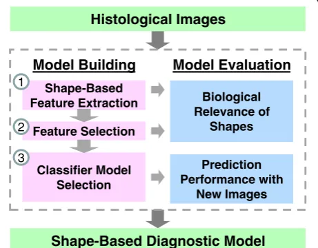
We develop an automatic histological image classification system that uses biologically interpretable shape-based features. These features capture the distribution of shape patterns, described by Fourier shape descriptors, in differ-ent stains of a histological image. We use this system to classify hematoxylin and eosin (H&E) stained renal tumor images and assess its classification performance by com-paring it to methods based on textural, morphological, and topological features.

The application of this system to cancer is important because, despite progress in treatment (e.g., early diag-nosis, reduction of mortality rates, and improvement of

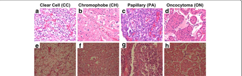
survival), cancer is still a major health problem in the United States. Specifically, it is estimated that there were 60,920 new kidney and renal pelvis cancer cases in the United States in 2011, resulting in 13,120 deaths [1]. Successful prognosis or treatment of renal cell carcin-oma (RCC) depends on disease subtype, each of which exhibits distinct clinical behavior and underlying genetic mutations [2]. Thus, it is important to accurately deter-mine the subtype of an RCC patient from among the most common subtypes: clear cell (CC, 70% of cases), papillary (PA, 15%), and chromophobe (CH, 5%) [3]. In addition, it is also important to identify benign renal tumors, the most common of which are the renal oncocytomas (ON, 5% of cases). Figure 1 shows typical examples of H&E-stained renal tumor images. Pathologists, guided by the World Health Organization (WHO) system, manually classify renal tumors using light microscopy based on typical features [3]. Even though the WHO sys-tem is capable of classifying typical examples, some cases

* Correspondence:[email protected] 1

Department of Electrical and Computer Engineering, Georgia Institute of Technology, Atlanta, GA, USA

2

Department of Biomedical Engineering, Georgia Institute of Technology and Emory University, Atlanta, GA, USA

Full list of author information is available at the end of the article

are more difficult. For example, ON and CH are often confused because both have granular cytoplasm. CH and CC can also be confused because both have prominent cell membranes. Moreover, there are two reported subtypes of PA that have varying visual appearance [3]. Thus, a pathologist’s diagnosis may be subjective.

Over the last decade, several automatic or automated systems have been developed to aid histological cancer diagnosis and to reduce subjectivity. All of these systems attempt to mimic pathologists by extracting features from histological images. Some important features include color, nuclear shape, fractal, textural gray-level co-occurrence matrices (GLCM), wavelets, and topological, among others [4,5]. Several diagnostic systems for renal cell carcinoma (RCC) are good examples of the utility of these features. For example, Chaudry et al. proposed a system using textural and morphological features with automated region-of-interest selection for RCC subtype classification [6,7]. Waheed et al. performed a similar analysis but included fractal as well as textural and mor-phological features [8]. Choi et al. extended the morpho-logical analysis to three-dimensional nuclei and applied their system to RCC grading [9]. In addition to morpho-logical features, Francois et al. used cell kinetic features in their RCC grading system [10]. Finally, Raza et al. used a scale invariant feature transform (SIFT) method to classify RCC subtypes [11]. Despite the success of these systems in terms of diagnostic accuracy, widespread use of these systems is limited by a lack of feature interpretability. Some researchers have provided visual interpretation of features. For example, some topological features have been related to the amount of differentiation in varying cancer grades [12]. In contrast, pathologists may not be receptive to, or confident in, features such as wavelet or fractal representations of images because they are not easy to interpret biologically. Moreover, most existing systems exploit morphological properties of nuclear shapes and

ignore cytoplasmic and glandular structures despite evidence of their utility [13]. Thus, methods based on a holistic view of shapes and colors may more accurately reflect the process by which a pathologist interprets a renal tumor image [3].

Fourier shape descriptors, described by Kuhl and Giardina [14] have been reported to be very useful as shape descriptors. They are highly robust to high frequency noise because of their ability to reject higher harmonic shape descriptors. Researchers have used Fourier shape descriptors for various medical imaging applications, including shape-based vertebral image retrieval [15], and classification of breast tumors [16]. The medical images involved in these studies typically have definite shapes with consistent landmarks. In addition, researchers have used Fourier shape descriptors for analyzing the shapes of nuclear structures [17-19]. Histological images, however, lack such landmarks and they tend to exhibit multiple highly variable shapes. As such, it is difficult to compare histological images using common techniques such as template matching with an image atlas [20] or using shape-based similarity measures after registration of the shapes in a histological image [21]. Therefore, in order to characterize and compare histological images in terms of shapes, we quantify the distribution of shape patterns in an image using Fourier shape descriptors.

models based on traditional histological image features. We show that Fourier shape-based features (1) are capable of classifying H&E-stained renal tumor histological images, (2) out-perform or complement traditional histological image features used in existing automated systems, and (3) are biologically interpretable.

Methods Image datasets

We perform this study on hematoxylin and eosin (H&E) stained histological RGB image datasets acquired from renal tumor samples of patients. In this study, we use two separately acquired datasets: dataset A and dataset B. Both datasets consist of photomicrographs of deidentified renal tumor specimens, derived from human patients. Research was conducted in compliance with the Helsinki Declaration. Tumor specimens were obtained through protocols approved by the Emory University Institutional Review Board, in which patients provided informed consent for residual tumor tissue to be stored in a university tissue bank. Administrators of the tissue bank provided deidentified tissues and associated clinical data (scrubbed of personal health identifiers), to the investigators of this research project. The IRB protocols pertaining to this research project are Emory IRB00045858/1214-2003 and 255–2002. Refer to Figures 1a-d and Figures 1e-h for

samples of images in dataset A and dataset B, respectively. After acquisition at constant magnification, a clinician se-lected 1600 × 1200-pixel portions from whole-slide images and a pathologist assigned each image to a renal tumor subtype. Dataset A contains 48 images with 12 images of each subtype while dataset B has 55 images including 20 chromophobe (CH), 17 clear cell (CC), 13 papillary (PA), and 5 oncocytoma (ON) subtypes. Dataset B has samples with nuclear grade varying from 1 to 4. In total, we analyze 103 renal tumor H&E images.

Automatic color segmentation of the renal tumor images requires an additional reference dataset. The reference dataset need not be the same tissue type. How-ever, the staining protocol should be the same as that of the renal tumor images. We use an H&E stained dataset of 50 randomly selected ovarian cancer images from the NIH Cancer Genome Atlas (TCGA) repository [22]. We use 1024 × 1024-pixel cropped portions of the original slide images. As references, these images are segmented by an expert user with the aid of a user-interactive system [23]. We then use these color-segmented reference images to automatically segment the renal tumor images as described in the following section.

Automatic color segmentation

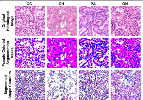
H&E staining of a renal tumor histological image en-hances three colors: blue-purple, white, and pink. These colors correspond to specific cellular structures. Baso-philic structures containing nucleic acids—ribosome and nuclei—tend to stain blue-purple; eosinophilic intra- and extracellular proteins in cytoplasmic regions tend to stain bright pink; empty spaces the lumen of glands do not stain and tend to be white. In order to isolate shapes corresponding to these cellular structures, we segment the three colors of every image using an automatic color segmentation method [23].

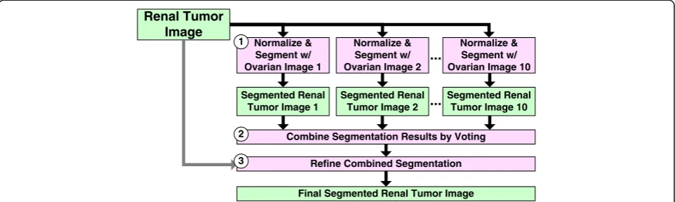
We use two batches of renal tumor images with very different stain colors. Batch-related variation in stain colors is a common problem in histological image analysis. As such, we use a robust automatic color segmentation system (Figure 3). Briefly, our system incorporates knowledge from pre-segmented reference im-ages (the ovarian cancer imim-ages) to normalize and segment renal tumor images. In order to make our system robust to the choice of reference image, we normalize and segment each renal tumor image using 10 ovarian cancer reference images (Figure 3, Step 1). We select 10 optimal ovarian cancer reference images from a set of 50 ovarian cancer images using the methodology described by [23]. The segmentation process first normalizes renal tumor image colors to the reference image colors, and then classifies the pixel into one of three groups (nuclei, cytoplasm, or lumen). Pixel classification is performed using a three-class linear discriminant classifier (LDA). We train the classifier Feature Selection

Shape-Based Diagnostic Model Histological Images

Shape-Based Feature Extraction

Classifier Model Selection

Model Evaluation

Biological Relevance of

Shapes

Prediction Performance with

New Images Model Building

1

2

3

using colors and labels in the reference image and classify pixels in the normalized renal tumor images.

The 10 segmentation labels for each pixel (one for each ovarian reference image) are combined using a voting scheme (Figure 3, Step 2). Voting chooses the segmentation label most frequently assigned to a pixel as its preliminary label.

The preliminary labels obtained by classification and voting are good approximations of the ground truth labels, but we further refine this segmentation using the LDA classifier (Figure 3, Step 3). This step trains the LDA classifier using colors from the original renal tumor image (before normalization) and using preliminary labels. The trained classifier is then used to re-classify all pixels in the renal tumor image. Intuitively, this is a post-processing step that ensures that the color group-ings are separable in the original sample image color space, and that any color distortion introduced by normalization is removed. Figure 4 illustrates some color segmentation results. Compared to the ground truth, (expert user-interactive segmentation) the overall segmentation accuracy is greater than 89%.

After segmentation, we extract a binary mask for each stain and apply morphological operations to the binary mask to connect broken boundaries and separate over-lapping objects. Namely, we dilate objects in the nuclear mask with a circular structural element with a two-pixel radius and erode objects in the cytoplasmic and glandular masks with a circular structural element with a three-pixel radius. Finally, from all binary masks, we remove small noisy regions with area less than five pixels and extract outer boundaries of the remaining connected objects for further analysis.

Shape descriptors

We use Fourier shape descriptors to represent shape contours. If we represent each shape contour using

parametric equations, (x(t), y(t)), the Fourier series ex-pansion for the one-dimensional periodic function x(t) andy(t) is given by

x tð Þ ¼A0þ

X1

n¼1 ancos

2nπt

T þbnsin

2nπt T

y tð Þ ¼C0þ

X1

n¼1 cncos

2nπt

T þdnsin

2nπt T

where n is the number of harmonics. We estimate the Fourier coefficients A0, C0, an, bn, cn, and dn by the formulas illustrated in [14]._A0and C0correspond to the location of a shape, so we do not consider them as shape descriptors. an, bn, cn, and dn are the shape descriptors that have commonly been used for shape discrimination [16,24] and shape retrieval [15,25] applications in 4*_N dimensional space, whereNis the number of harmonics. However, we are classifying images based on the distri-bution of multiple shapes within the images and not based on individual shapes. Therefore, we quantify the distributions of an individual descriptor over all the shapes in an image mask and use these distributions as shape-based features for classification (described in the next section). The distribution of four coefficients,an,

bn, cn, dn, for harmonic n cannot be used separately because they jointly describe an ellipse:

xnð Þ ¼θ ancosθþbnsinθ

ynð Þ ¼θ cncosθþdnsinθ

where

θ¼2nπt T

However, using both the semi-major and semi-minor axis lengths of ellipses, we can capture the shape Renal Tumor

Image

Normalize & Segment w/ Ovarian Image 1

Segmented Renal Tumor Image 1

Segmented Renal Tumor Image 2

Segmented Renal Tumor Image 10

Combine Segmentation Results by Voting

Final Segmented Renal Tumor Image Refine Combined Segmentation

Normalize & Segment w/ Ovarian Image 2

Normalize & Segment w/ Ovarian Image 10

...

...

1

2

3

patterns. We quantify semi-major and semi-minor axis lengths as follows. The magnitude of the ellipse phasor is given by

rð Þ ¼θ

ffiffiffiffiffiffiffiffiffiffiffiffiffiffiffi

x2

nþy2n q

ð1Þ

We can locate the extrema of this phasor magnitude by differentiating equation (1) and solving for its root. The resulting solution forθis

θn¼ 1 2 tan

1 2ðanbnþcndnÞ

a2

nþc2nb2nd2n

;where 0≤θ≤π ð2Þ

Now, asr(θ) describes an ellipse,θngives the location of either the major or minor axis while the other axis is given byθ_nþπ=2. Therefore, semi-major and semi-minor

axes are given by

rn1¼ max rð Þθn ;r θnþπ 2

ð3Þ and

rn2¼ min rð Þθn ;r θnþπ 2

ð4Þ

r1

n and r2n capture the magnitude of a shape’s variation in thenthharmonic. For n= 1,rn1 and rn2 encode the size of the shape. Forn> 1,r1

nandr2nencode the complexity of the shape. For simpler shapes, i.e. closer to an ellipse, r1

n and r2

n quickly reduce to zero, with increasingn,while for more complex shapes, they reduce slowly. Therefore, _r1

n and r2

n approximately describe a shape and its complexity (similar to the original Fourier coefficients:an-dn), but can be separated while quantifying the amount of variation in a particular harmonic. Therefore, instead of using individual descriptors, we use the semi-major (greater ofr1

norr2n) and semi-minor axis lengths as our shape descriptors. For quantifying shapes, we capture information using up to 10 harmonics to determine how many harmonics are sufficient for image representation and subtype classification.

Figure 4Color segmentation results and shape contours in three masks for four renal tumor subtypes: clear cell (CC), chromophobe (CH), papillary (PA), and oncocytoma (ON).First row: original histological renal tumor subtype images;second row: pseudo colored

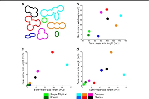
Figure 5 illustrates shape axes descriptors for synthetic-ally generated clusters of nuclei. In Figure 5b, for the 1st harmonic, axes features describe size and eccentricity of a shape. For higher harmonics axis lengths encode detail about the shape. Therefore, in Figure 5c and Figure 5d, for the 2nd and 3rd harmonics, simple (closer to an ellipse) shapes (such as the green shapes) have axis lengths close to zero while all other shapes have larger axis lengths.

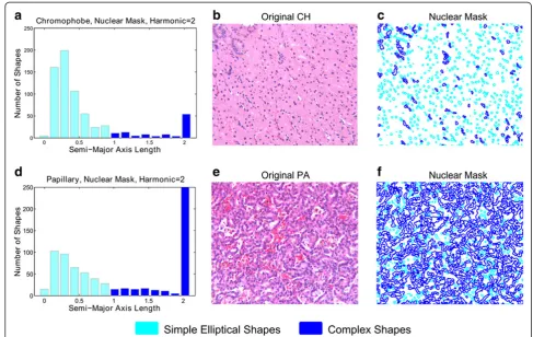
Figure 6 illustrates the ability of the axis length distribu-tion to capture the shape profile of an image. In this figure, we are considering nuclear (blue) mask shapes for two RCC subtypes: chromophobe and papillary. Figures 6a and d represent the distribution of major axis length at harmonic two in the shapes of the images in Figures 6b and e, respectively. The second harmonic captures the complexity of the shape approximation. Although these histograms do not capture the spatial positions of shapes in histopathological images, spatial positions are not useful because the positions of objects (e.g., nuclei) in

histopathological images are highly variable from image to image. Instead, these histograms capture the overall pro-portion of complex or simple shapes in a histopathological image. Thus, for complex shapes like papillary nuclear clusters (resulting from overlapping nuclei in histology), the major axis length of the second harmonic tends to have higher values compared to that of simpler shapes like individual circular nuclei. Consequently, the distribution of shape major axis lengths in papillary images is different from that of chromophobe images. In Figure 6c and Figure 6f corresponding to the histograms in Figure 6a and Figure 6d, respectively we have outlined, in cyan, shapes with values of major axis length that fall in the lower seven bins. Shapes with values of major axis length falling in the upper eight bins are outlined in blue. We can observe that the chromophobe image (Figures 6a, b and c) has a dominant pattern of simple shapes as compared to the papillary image (Figures 6d, e and f ). As described in the next section, discretization of axis lengths of all shapes

in an image is the basis for representing a histological image as a multi-feature observation.

Discretization of shape descriptors

In order to develop a classification system, we represent each image as a single observation with a fixed number of features. Due to the variable number of shapes in each image, we quantify the distribution of shape descriptors (axis lengths) to create a“shape profile”, represented as a histogram. We determine the dynamic range of each histogram by computing interquartile distances of shape descriptor distributions from the training set. Interquartile distance is the distance between the 25th and 75th percentiles of a distribution [26]. Mathematically, _Rc;m_n is the distribution of axis lengths over all shapes in all images in the training dataset for a particular combination of harmonic (n), axis type (c) and mask (m). Let function

fP(R) return thepth percentile of distributionR, then the interquartile distance (IQD) is given by

IQD Rð Þ ¼f0:75ð Þ R f0:25ð ÞR ð5Þ

Using equation (5), weRc;m_n :

Lc;mn ¼ max 0; f0:5 Rc;m_n

2IQD Rc;mn

ð6Þ

Unc;m¼f0:5 Rc;m_n

þ2IQD Rc;mn

ð7Þ

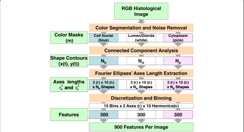
where L, U are the lower and upper bounds of the range, respectively. Outliers bin into the edges of the histogram and may be informative features. Axis lengths are always positive, therefore the lower bound of the range is forced to be greater than or equal to zero. Figure 7 illustrates the data flow from a histo-logical RGB image to a list of 900 features. The pro-cedure is as follows:

1. Generate a binary mask for each color in the histological image. We use three colors for H&E stained RCC images: blue (nuclear), white (no-stain/ glandular), and pink (cytoplasmic).

2. Extract contours for all shapes in a mask after connected component analysis.

3. Extract axis lengths for Fourier ellipses (r_n1andr_n2) for the first 10 harmonics (n). This will give us 2*10 variables for each shape.

4. For each harmonic (n), axis type (c), and mask (m), perform a binning procedure (Figure8). We generate 20 histograms for each mask. We use 15 bins and a range determined byLc;m_n andU_nc;mas previously described.

5. Combine histogram frequency from the three masks to generate a list of 900 shape-based features

There are a number of advantages in using discretization rather than Euclidian distance to compare images. First, the axes of shapes that are similar, but per-haps not identical, fall into the same histogram bin. Similar histogram frequencies can be interpreted as a similarity of shapes between images. Second, bins sensi-tive to noise or outlier shapes in any sample will be rejected during feature selection. Finally, discriminating features can be components corresponding to multiple types of shapes rather than components corresponding to the most prominent characteristic shape.

Traditional features

Traditional features in computer-aided diagnosis include texture, morphological, topological, and nuclear. In order to compare shape-based features to these traditional features, we extract additional features from histological renal tumor images.

For texture, we have two sets of features: Gray-Level Co-occurrence Matrix (GLCM) and wavelet. For GLCM features, we extract a 16 × 16 GLCM matrix for each gray-scale tissue image with 16 quantization levels [27]. Using this matrix, we extract 13 texture properties includ-ing contrast, correlation, energy (angular second moment), entropy, homogeneity (inverse difference moment), vari-ance, sum average, sum varivari-ance, sum entropy, difference variance, difference entropy, and two information measures for correlation. These features are reported to successfully capture texture properties of the image and are very useful in automated cancer grading [12,27,28].

For wavelet features, we perform three-level wavelet (db6) packet decomposition [29] of the gray-level tissue image and extract energy and entropy [30] of 84 coefficient matrices (level 1, 2 and 3), producing 168 features. Wavelet features capture texture properties of an image.

RGB Histological Image

Lumen/Glands (white)

Cytoplasm (pink)

Color Segmentation and Noise Removal

Cell Nuclei (blue)

Connected Component Analysis

N_b N_w N_p

Fourier Ellipses’ Axes Length Extraction

2 (r) x 10 (n) x NbShapes

2 (r) x 10 (n) x NwShapes

2 (r) x 10 (n) x NpShapes Color Masks

(m)

Shape Contours (x(t), y(t))

Axes lengths and

1 n

r r_n2 x NbShapes x NwShapes x NpShapes

Discretization and Binning

15 Bins x 2 Axes (r) x 10 Harmonics(n)

300 300 300

900 Features Per Image Features

and

1 n

r r_n2

Figure 7The data flow for extraction of 900 shape-based features from a histological image.First, we segment the RGB histological image based on stains: blue (nuclei), pink (cytoplasm), and white (no-stain/gland). Then based on segmented results, we generate three binary masks corresponding to three stains (blue:b, white:w, pink:p). For each mask, we obtain the contour for all shapes after noise filtering using connected component analysis. Nmis number of shapes inmmask, wherem∈{b,w,p}. We then extract shape axes descriptors (2 axes*10

For morphological features, we use color-GLCM, a method proposed by Chaudry et al. to classify renal tumor subtypes. This method generates a four-level gray-scale image from four color stains in H&E-stained images [7]. The four colors resulting from H&E-stained images (blue, white, pink, and red) correspond to segmented regions of nuclei, lumen, cytoplasm, and red blood cells. We then extract a 4 × 4 GLCM matrix for the gray-scale image. We extract 21 features from this matrix including 16 elements of the 4 × 4 GLCM matrix, contrast, correl-ation, energy (angular second moment), entropy, and homogeneity (inverse difference moment). These features capture morphological features of the image such as stain area and stain co-occurrence properties.

For topological features, we use a graph-based method. Several researchers have proposed graph-based features to capture the distribution of patterns in an image. Biologically, these features capture the amount of differenti-ation (related to cancer grade) in a histological image. We morphologically erode our nuclear mask to separate nuclear clusters and use their centroids (nuclear centers) for this analysis. First, we create a Voronoi diagram from these centers and then calculate area and perimeter of each region and all side-lengths. We then calculate mean, minimum, maximum, and disorder of the distribution to produce 12 features [12]. The disorder, D, of a distribution, r, is given by

D r

ð Þ ¼

1

1

þ

=

μr

, where σr and

μrare standard deviation and mean of r, respectively [31]. Second, we calculate the area and side lengths of the Delaunay triangles and extract statistics similar to those of the Voronoi diagram to produce eight more features. Last, we calculate side lengths of the minimum spanning tree and extract the same statistics to produce four more features. In total, we extract 24 topological features.

For nuclear features, we extract nuclear count and elliptical-shape properties, which have proven to be

useful for renal carcinoma subtyping and grading [32]. For segmenting nuclear clusters, we use an edge-based method with three steps: concavity detection, straight-line segmentation, and ellipse fitting [33]. We describe each elliptical nucleus using area, major-axis length, minor-axis length, and eccentricity. We then calculate mean, mini-mum, maximum and disorder of the distribution of these descriptors to produce 16 features. In total, including nuclear count, we extract 17 nuclear features.

We combine the GLCM (13 features), color-GLCM (21), wavelet (168), topological (24), and nuclear (17) features to produce a set of 243“Combined Traditional” features. Finally, we combinethe“Combined Traditional” (243) and “Shape” (900) features to a produce a set of 1143“All”features.

Feature selection and classification

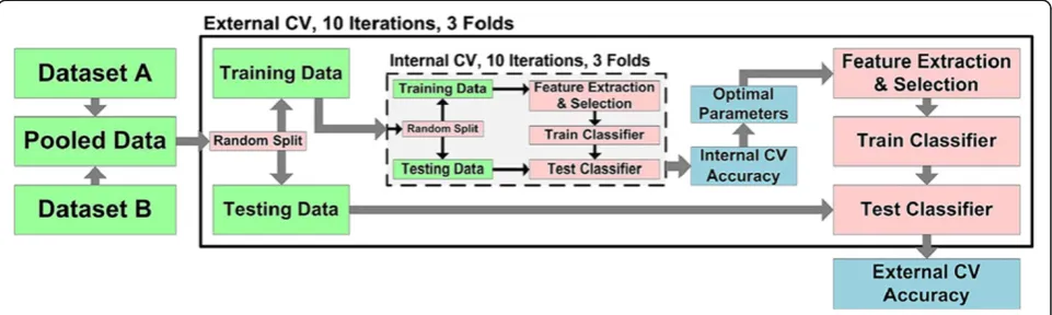
For validation, we combine datasets A and B, then randomly split them into two new training and testing datasets with balanced sampling from both datasets. We perform a three-fold split, in which two folds form the training set while one fold forms the testing set. Each fold acts as a testing set once, resulting in three train-ing–testing sets. We perform 10 iterations of this split to estimate the variance in performance. Thus, there are 30 training–testing sets in the external cross-validation (CV) that produces the final classification accuracy. For each of the 30 training sets, we perform an additional three-fold, 10 iterations of CV to choose an optimal set of classifier and feature selection parameters. This forms the internal CV of a nested CV (Figure 8).

we use the hierarchy illustrated in Figure 9. Each node in the hierarchy is independently optimized such that, for each binary comparison, we choose a set of model parameters (i.e., classifier as well as feature selection parameters). We consider 224 SVM classifier models including 14 kernel types (linear or radial with the gamma parameter ranging from 22, 21, 20to 2-10) and 16 cost values (2-5, 2-4, 2-3to 210) [35,36]. We considered the following feature sizes for different features (e.g., starting feature size:feature step size:ending feature size):

1. GLCM (1:1:13) 2. Color-GLCM (1:1:21) 3. Wavelet (1:5:166) 4. Topological (1:1:24) 5. Nuclear (1:1:17)

6. Combined Traditional (1:6:243) 7. Shape and All (5:5:180)

We choose the feature size step such that the total number of feature sizes is approximately 40. For Shape and All features we also consider number of harmonics (n= 2 to 10) as a feature selection parameter. We choose the simplest model with a CV accuracy within one standard deviation of the best performing model [37]. In choosing the simplest model, we give preference to the linear SVM kernel over the radial SVM kernel and lower

values of gamma for the radial SVM kernel, SVM cost, number of harmonics, and feature size.

We select features using a feature ranking technique called mRMR (Minimum Redundancy Maximum rele-vance) [38]. MRMR selects a set of features that maximizes mutual information between class labels and each feature in the set; and minimizes mutual information between all pairs of features in the set. Our features are continuous and, as suggested by Ding et al., we use Mutual Information Quotient (MIQ) optimization after discretization using the following transform:

k0 ¼ 1

0 1

k<μkσk=2

μkσk=2≤k≤μkþσk=2

k>μkþσk=2 8 < : 9 = ;

where k’ is the transformed feature k, μk and σk are the mean and standard deviation of feature kover all samples in the training dataset, respectively.

Results and discussion

Shape-based features discriminate renal tumor histological images

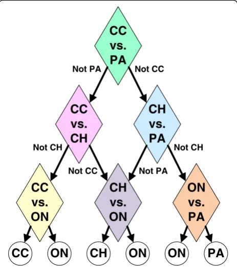
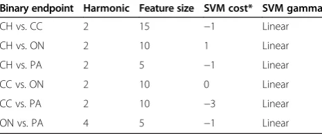
Fourier shape-based features are capable of classifying histological renal tumor subtype images with high accuracy and simple classification models. Table 1 lists the shape-based prediction performance of the multi-class renal tumor classifier (using a Directed Acyclic Graph, DAG, classifier [34]) as well as that of each binary comparison (discrimination of every pair of subtypes). The shape-based multi-class classifier predicts the subtypes of renal tumor images with an average accuracy of 77%. The average prediction accuracy for each binary comparison ranges between 83%-96%. Moreover, the classification model for each binary comparison is fairly simple, i.e., each model uses (1) shapes described by lower harmonics, (2) small feature size, and (3) a linear SVM with low cost (Table 2). Refer to Additional file 1 for detailed classifier model selection results.

We use nested cross-validation (CV) to select predic-tion model parameters and to evaluate these predicpredic-tion models on independent data. The nested CV procedure

CC

vs.

PA

CC

vs.

CH

CH

vs.

PA

CC

vs.

ON

CH

vs.

ON

ON

vs.

PA

CC

ON

CH

ON

ON

PA

Figure 9A multi-class hierarchy of binary renal tumor subtype classifiers, also known as a directed acyclic graph (DAG) classifier.The overall accuracy of the DAG classifier can be optimized by independently optimizing each binary comparison.

Table 1 Predictive performance of shape-based features

Endpoint Inner CV accuracy External CV accuracy

DAG N/A 0.77 ± 0.03

CH vs. CC 0.83 ± 0.03 0.83 ± 0.05

CH vs. ON 0.83 ± 0.02 0.84 ± 0.04

CH vs. PA 0.97 ± 0.01 0.96 ± 0.02

CC vs. ON 0.90 ± 0.02 0.90 ± 0.07

CC vs. PA 0.96 ± 0.01 0.95 ± 0.04

includes 10 iterations of three-fold external CV with 10 iterations of three-fold internal CV. Although there is some variance across the iterations of CV, Figure 10 shows that mean internal CV is a good estimate of mean external CV for each of the binary comparisons. Each point in Figure 10 corresponds to an iteration of external CV for each binary comparison. The horizontal position of each point is internal CV accuracy averaged over 10 iterations and three folds. The vertical position of each point is external CV accuracy averaged over three folds. Classifier model parameters for each point are selected from among 72,576 models consisting of 36 feature sizes, 14 types of SVM classifiers (linear SVM and radial basis SVM classifiers over 13 different gammas), 16 SVM cost values, and 9 values for the number of harmonics. The optimal parameter set for each classifier model corresponds to the simplest model (i.e., smallest feature size, smallest cost, smallest gamma, and smallest number of harmonics) within one standard deviation of the best performing model. This high concordance of internal CV and external CV performance indicates that internal CV performance is predictive of external CV performance and classifier models generated from shape features are robust and will perform similarly for future samples. Moreover, the binary comparisons discriminating CH vs. PA, CC vs. ON, CC vs. PA, and ON vs. PA tend to result in high performance (> 90%) while the binary comparisons discriminating CH vs. CC and CH vs. ON result in moderate performance (~83-84%). We describe the reasons for these observations below.

CC and PA are the most prevalent subtypes of RCC and are generally the easiest for pathologists to visually identify. Consequently, discriminating shape-based features for these classes are easy to identify, resulting in high classification performance. One exception, however, is the CH vs. CC comparison. CH is known to exhibit some CC properties such as clear cytoplasm. As a result, the prominent feature for the CC subtype is sometimes not sufficient for accurate classification of CC and CH. Moreover, the ON renal tumor subtype is histologically and genetically very similar to the CH RCC subtype, despite the fact that ON is a benign tumor whereas CH is a carcinoma [39]. This

similarity explains the moderate performance of the CH and ON binary classifier.

Shape-based features out-perform or complement traditional histological features

Table 3 shows that, in comparison to five traditional feature sets, classification of renal tumor subtypes based on shape-based features performs well. In fact, the performance of shape features is similar to the combined traditional features, which includes texture, topological and nuclear properties. In some cases, combining shape-based features with traditional features (i.e.,‘All’features) improves prediction performance, indicating that shape-based features can complement traditional features. Table 3 lists the means and standard deviations over 10 iterations of external CV for each binary comparison as well as for the multi-class DAG classifier. Figure 11 shows the contribution of each feature type to the classi-fication model when considering ‘All’ features. The box plots in Figure 11 represent the distribution of percent contribution of each feature type to a binary classifier over 10 iterations of external CV. We can make the following observations from Figure 11: 1) Shape features have a high (>55%) contribution for all binary endpoints, which indicates that the feature selection method ranks shape features higher than other features. The contribu-tion is comparatively lower for CH vs. CC, CH vs. ON, and CC vs. ON endpoints because other traditional features were also useful for these endpoints. 2) Nuclear features, which capture nuclear-shape properties, highly contribute to all six endpoints 2) In addition to shape features for the CH vs. ON endpoint, topological, nuclear and wavelet features also contribute to the prediction models, resulting in a 4% increase in accuracy compared to shape features alone. This indicates that, in addition to shape (Fourier and nuclear) properties, CH and ON differ in topological and wavelet properties. 3) Color GLCM performs very well for CC vs. PA classification. Thus, color GLCM is a major contributor for CC vs. PA classification, resulting in a 2% increase in accuracy. Shape-based features are biologically interpretable Figure 12 illustrates the biological interpretability of shape-based features for each renal tumor subtype. In order to visualize the biological significance of the features identified by our feature selection method, we overlay the top discriminating shapes on the images of renal tumor subtypes for each binary comparison. Feature selection identifies individual shape axes and not entire shapes. Thus, discriminating shapes are shapes with axes values that have been discretized into a bin corresponding to a highly ranked feature. For each binary comparison, we identify all shapes in an image that have Fourier axes values corresponding to the top 25 features.

Table 2 Frequently selected model parameters for each binary comparison

Binary endpoint Harmonic Feature size SVM cost* SVM gamma

CH vs. CC 2 15 −1 Linear

CH vs. ON 2 10 1 Linear

CH vs. PA 2 5 −1 Linear

CC vs. ON 2 10 0 Linear

CC vs. PA 2 10 −3 Linear

ON vs. PA 4 5 −1 Linear

These shapes are selected using features from all images. We set the“number of harmonics”parameter equal to the most selected value during the cross-validation (Table 2). We selectively color the shapes based on“over expression”, or increased relative frequency for particular subtypes. Shapes highlighted in green occur more frequently in CC; yellow shapes occur more frequently in PA; blue shapes occur more frequently in CH; and black shapes occur more frequently in ON. We interpret the biological significance of highlighted shapes for each binary comparison.

Histopathological features of the CC subtype include clear cytoplasm, compact alveolar, tubular, and cystic architecture leading to distinct cell membranes [3]. Comparing CC to PA and ON, we see that clear cytoplasm (no-stain/glandular (white) mask region, outlined with

green) is the primary distinguishing characteristic that is noticeably less frequent in PA and ON. On the other hand, because CH images tend to also exhibit halos resembling clear cytoplasm, the distinguishing features between CC and CH are distinct cell membranes (small cytoplasmic (pink) mask areas outlined with green between larger no-stain/glandular (white) mask areas) that are more frequent in CC compared to CH. Similarity in halos and clear cytoplasm shapes is possibly the reason for low accuracy in the CH vs. CC binary classification.

Features of the PA subtype include scanty eosinophilic cytoplasm and a papillary (i.e., finger-like) pattern of growth resulting in long, complex clusters of nuclei [3]. In all comparisons with the PA subtype, complex clusters of nuclei are the dominant distinguishing feature and are

0.7 0.75 0.8 0.85 0.9 0.95 1

0.7 0.75 0.8 0.85 0.9 0.95 1

Accuracy of Internal Cross Validation

Accuracy of External Cross Validation

Classfication Accuracy Using Shape−Based Features

CH vs. CC CH vs. ON CH vs. PA CC vs. ON CC vs. PA ON vs. PA

Figure 10Cross-validation estimates the prediction performance of shape-based classification models on independent samples.Scatter plot of inner CV vs. external CV average validation accuracy values over 10 external CV iterations for six pair-wise renal tumor subtype

comparisons: CH vs. CC, CH vs. ON, CH vs. PA, CC vs. ON, CC vs. PA, and ON vs. PA. The plotted performance value for each iteration is the average performance over three folds (for external CV) or over 10 iterations and three folds (for internal CV). The optimal classifier model parameters (one set for each point) are selected in the inner CV from a possible set of 72576 models consisting of 36 feature sizes, 14 types of classifiers (linear SVM and radial basis SVM classifiers with 13 different gammas), 16 cost values and 9 harmonic numbers.

Table 3 Classification accuracy of features in external CV*

Endpoint GLCM Color GLCM Wavelet Topological Nuclear Combined

traditional

Shape (Proposed)

All

DAG 0.57 ± 0.04 0.67 ± 0.02 0.52 ± 0.06 0.50 ± 0.03 0.66 ± 0.03 0.79 ± 0.04a _{0.77 ± 0.03}b _{0.78 ± 0.03}c

CH vs. CC 0.75 ± 0.05 0.77 ± 0.05 0.74 ± 0.05 0.74 ± 0.05 0.76 ± 0.06 0.81 ± 0.03 0.83 ± 0.05 0.82 ± 0.05

CH vs. ON 0.76 ± 0.05 0.68 ± 0.06 0.67 ± 0.05 0.72 ± 0.05 0.79 ± 0.05 0.86 ± 0.05 0.84 ± 0.04 0.88 ± 0.04

CH vs. PA 0.85 ± 0.04 0.95 ± 0.02 0.86 ± 0.05 0.80 ± 0.04 0.91 ± 0.04 0.94 ± 0.02 0.96 ± 0.02 0.96 ± 0.03

CC vs. ON 0.74 ± 0.06 0.78 ± 0.06 0.63 ± 0.03 0.77 ± 0.07 0.93 ± 0.04 0.93 ± 0.04 0.90 ± 0.07 0.91 ± 0.05

CC vs. PA 0.78 ± 0.06 0.97 ± 0.04 0.69 ± 0.09 0.59 ± 0.07 0.76 ± 0.07 0.95 ± 0.05 0.95 ± 0.04 0.97 ± 0.03

ON vs. PA 0.74 ± 0.07 0.86 ± 0.06 0.74 ± 0.07 0.65 ± 0.04 0.96 ± 0.03 0.97 ± 0.03 0.93 ± 0.04 0.92 ± 0.04

generally more prominent in PA (nuclear (blue) mask areas outlined with yellow). The frequency of nuclear shapes in ON appears to be similar to that of PA. However, the nuclear clusters in PA are generally larger and more irregular due to the clustering, resulting in different Fourier shape axes values.

Histopathological features of the CH subtype include wrinkled nuclei with perinuclear halos [3]. When compar-ing CH to PA or ON, our feature extraction and selection method identifies these halos (no-stain/glandular (white) mask areas, outlined with blue). In addition, single nuclei become dominant when comparing CH to PA.

Histopathological features of the ON subtype include granular cytoplasm with round nuclei, usually arranged in compact nests or microcysts [3]. These round nuclei appear to be dominant in ON when compared to other subtypes. It can be observed that dominant features for both CH and ON are present in the opposite subtype as well. Hence, the difficulty in distinguishing the two subtypes.

Limitations and computational complexity of shape-based features

Some limitations of shape-based features for histological image classification depend on the specific biological application. Shape-based features may not be suitable for cases in which the primary discriminating features are not based on shapes. For example, in cancer grad-ing applications, topological and texture properties may be more useful than shape-based features. More-over, as we have seen the results of Table 3 and Figure 11, shape-based features may not capture all of the important distinguishing information. For example,

in the case of the CH vs. ON endpoint, the addition of texture and wavelet features to shape-based features increases prediction performance by 4%. In addition, for the CC vs. PA endpoint, inclusion of the GLCM texture features increases prediction performance by 2%. Thus, shape-based features are limited to clinical prediction applications that are inherently shape-based, but, in such cases, may be used to complement other non-shape-based features.

The computational complexity of shape-based features is higher than those of traditional histological feature extraction and analysis methods, but should not prevent implementation in a clinical setting. To convert a RGB histological image (1600x1200 pixel portions) into 900 shape-based features (Figure 7), a desktop computer (Intel Xeon E5405 quad-core processor, 20 GB RAM) requires an average of 74.96 seconds. Compared to some histological image features, this processing time is high. However, the processing time depends on the number of harmonics used for representation and the number of shapes in an image. We have reported the processing time for extracting features from the first ten harmonics. However, in practice, we have observed that all opti-mized models use less than five harmonics. Optimization of these parameters to identify a predictive model can be time consuming depending on the size of the training set. However, in a clinical setting, such a model would only need to be optimized once, and then periodically updated with new patient data. In a clinical scenario, a pathologist that requires a histological diagnosis for a patient would submit a few image samples from a tissue biopsy to a pre-optimized prediction system. 0

0.1 0.2 0.3 0.4 0.5 0.6 0.7 0.8 0.9 1

CH vs. CC CH vs. ON CH vs. PA CC vs. ON CC vs. PA ON vs. PA

Renal Tumor Subtype Comparisons

Percent Contribution

Percent Contribution of Various Features to Classification Model

GLCM Color−GLCM Wavelet Topological Nuclear Shape

Computational time for processing and predicting based on these image samples would be negligible compared to time required for biopsy, image acquisi-tion, and consultation with a pathologist.

Conclusions

We presented a novel methodology for automatic clinical prediction of renal tumor subtypes using shape-based fea-tures. These shape-based features describe the distribution of shapes extracted from three dominant H&E stain colors in renal tumor histopathological images. We evaluated the four-class prediction performance of shape-based classifica-tion models using 10 iteraclassifica-tions of three-fold nested CV.

The overall classification accuracy of 77% (average external CV accuracy) is favorable compared to previous methods that use traditional textural, morphological, and wavelet-based features. Moreover, results indicate that combining shape-based features with traditional histological image features can improve prediction performance. The bio-logical significance of the characteristic shapes identified by our algorithm suggests that this automatic diagnostic system mimics the diagnostic criteria of pathologists. We applied this methodology to renal tumor subtype prediction. However, the methodology may be extended to any histological image classification problem that traditionally depends on visual shape analysis by a Figure 12The top discriminating shapes for six binary endpoints correspond to pathologically significant shapes in histological renal tumor images.We identify the top 25 features selected for each binary comparison and highlight all shapes in the images that have any Fourier shape-descriptor axes lengths corresponding to these top features. We selectively color the shapes based on“over expression”or increased relative frequency for particular subtypes.Green shapes: occur more frequently in clear cell;yellow shapes: occur more frequently in papillary;

pathologist. Moreover, these shape-based features may be coupled with other image features to achieve higher diagnostic accuracy.

Additional file

Additional file 1:This file includes figures describing classifier model parameter space investigation.

Abbreviations

RCC: Renal cell carcinoma; CC: Clear cell; PA: Papillary; CH: Chromophobe; ON: Oncocytoma; mRMR: Minimum redundancy maximum relevance; DAG: Directed acyclic graph; CV: Cross-validation; GLCM: Gray-level co-occurrence matrix; DAG: Directed acyclic graph; LDA: Linear discriminant analysis; SVM: Support vector machine.

Competing interests

The authors declare that they have no competing interests.

Authors_’contributions

SK designed the image feature extraction methods (including color segmentation, shape descriptor extraction and discretization), contributed to the design of validation experiments and shape feature visualization, implemented all methods, and drafted the manuscript. JHP designed validation experiments and shape feature visualization, and contributed to the design of feature extraction methods. ANY provided all biological specimens and provided biological interpretation of informative shapes for each tumor subtype. MDW initiated the development of the automatic cancer diagnostic system, acquired funding to sponsor this multi-year effort, and directed the development of the shape-based analysis methodology and publication. All authors read and approved the final manuscript.

Acknowledgment

We thank Dr. Todd Stokes and Dr. Mitch Parry for their valuable comments and suggestions. This research has been supported by grants from NIH (Bioengineering Research Partnership R01CA108468, P20GM072069, and CCNE U54CA119338), Georgia Cancer Coalition, Hewlett Packard, and Microsoft Research.

Author details

1

Department of Electrical and Computer Engineering, Georgia Institute of Technology, Atlanta, GA, USA.2_{Department of Biomedical Engineering,} Georgia Institute of Technology and Emory University, Atlanta, GA, USA. 3_{Pathology and Laboratory Medicine, Emory University, Atlanta, GA, USA.} 4

Grady Health System, Atlanta, GA, USA.

Received: 15 March 2012 Accepted: 20 February 2013 Published: 13 March 2013

References

1. Siegel R, Ward E, Brawley O, Jemal A:Cancer statistics, 2011.CA Cancer J Clin2011,61(4):212–236.

2. Teloken PE, Thompson RH, Tickoo SK, Cronin A, Savage C, Reuter VE, Russo P:Prognostic Impact of Histological Subtype on Surgically Treated Localized Renal Cell Carcinoma.J Urol2009,182(5):2132–2136. 3. Eble J, Sauter G, Epstein J, Sesterhenn I:Pathology and genetics of tumours

of the urinary system and male genital organs.Lyon: IARC press Lyon; 2004. 4. Demir C, Yener B:Automated cancer diagnosis based on histopathological

images: a systematic survey.Tech Rep: Rensselaer Polytechnic Institute; 2005. 5. Gurcan MN, Boucheron LE, Can A, Madabhushi A, Rajpoot NM, Yener B:

Histopathological image analysis: A review.Biomed Eng, IEEE Rev2009, 2:147–171.

6. Chaudry Q, Raza SH, Sharma Y, Young AN, Wang MD:Improving renal cell carcinoma classification by automatic region of interest selection.In

BioInformatics and BioEngineering, 2008 BIBE 2008 8th IEEE International Conference on: 2008.Athens, Greece: IEEE; 2008:1–6.

7. Chaudry Q, Raza SH, Young AN, Wang MD:Automated Renal Cell Carcinoma Subtype Classification Using Morphological, Textural and Wavelets Based Features.J Signal Process Syst2009,55(1):15–23.

8. Waheed S, Moffitt RA, Chaudry Q, Young AN, Wang MD:Computer Aided Histopathological Classification of Cancer Subtypes.InBioinformatics and Bioengineering, 2007 BIBE 2007 Proceedings of the 7th IEEE International Conference on: 2007.Boston, United States: IEEE; 2007:503–508. 9. Choi HJ, Choi HK:Grading of renal cell carcinoma by 3D morphological

analysis of cell nuclei.Comput Biol Med2007,37(9):1334–1341.

10. François C, Moreno C, Teitelbaum J, Bigras G, Salmon I, Danguy A, Brugal G, van Velthoven R, Kiss R, Decaestecker C:Improving accuracy in the grading of renal cell carcinoma by combining the quantitative description of chromatin pattern with the quantitative determination of cell kinetic parameters.Cytometry B Clin Cytom2000,42(1):18–26. 11. Raza SH, Sharma Y, Chaudry Q, Young AN, Wang MD:Automated

classification of renal cell carcinoma subtypes using scale invariant feature transform.InEngineering in Medicine and Biology Society, 2009 EMBC 2009 Annual International Conference of the IEEE: 3_–6 Sept. 2009 2009.

Minneapolis, United States: IEEE; 2009:6687–6690.

12. Doyle S, Agner S, Madabhushi A, Feldman M, Tomaszewski J:Automated grading of breast cancer histopathology using spectral clustering with textural and architectural image features.InBiomedical Imaging: From Nano to Macro, 2008 ISBI 2008 5th IEEE International Symposium on: 2008.

Paris, France: IEEE; 2008:496–499.

13. Sertel O, Kong J, Catalyurek UV, Lozanski G, Saltz JH, Gurcan MN: Histopathological image analysis using model-based intermediate representations and color texture: Follicular lymphoma grading.J Signal ProcessSyst2009,55(1):169_–183.

14. Kuhl F, Giardina C:Elliptic Fourier features of a closed contour.Comput Graph Image Process1982,18(3):236–258.

15. Lee D, Antani S, Long L:Similarity measurement using polygon curve representation and fourier descriptors for shape-based vertebral image retrieval.In: SPIE Medical Imaging2003,2003:1283–1291.

16. Rangayyan R, El-Faramawy N, Desautels J, Alim O:Measures of acutance and shape for classification of breast tumors.IEEE Trans Med Imaging

1997,16(6):799–810.

17. Cukierski W, Nandy K, Gudla P, Meaburn K, Misteli T, Foran D, Lockett S: Ranked retrieval of segmented nuclei for objective assessment of cancer gene repositioning.BMC Bioinforma2012,13(1):232.

18. Yang L, Tuzel O, Chen W, Meer P, Salaru G, Goodell LA, Foran DJ: PathMiner: a Web-based tool for computer-assisted diagnostics in pathology.IEEE Trans Inf Technol Biomed2009,13:291–299.

19. Comaniciu D, Meer P:Cell Image Segmentation for Diagnostic Pathology. InAdvanced Algorithmic Approaches to Medical Image Segmentation.Edited by Suri JS, Setarehdan SK, Singh S. London: Springer; 2002:541–558. 20. Lao Z, Shen D, Xue Z, Karacali B, Resnick S, Davatzikos C:Morphological

classification of brains via high-dimensional shape transformations and machine learning methods.Neuroimage2004,21(1):46–57.

21. Berg AC, Berg TL, Malik J:Shape matching and object recognition using low distortion correspondences.InComputer Vision and Pattern Recognition, 2005 CVPR 2005 IEEE Computer Society Conference on: 2005 2005, Volume 21. San Diego, United States: IEEE; 2005:26–33.

22. McLendon R, Friedman A, Bigner D, Van Meir E, Brat D, Mastrogianakis G, Olson J, Mikkelsen T, Lehman N, Aldape K:Cancer Genome Atlas Research Network. Comprehensive genomic characterization defines human glioblastoma genes and core pathways.Nature2008, 455(7216):1061–1068.

23. Kothari S, Phan JH, Moffitt RA, Stokes TH, Hassberger SE, Chaudry Q, Young AN, Wang MD:Automatic batch-invariant color segmentation of histological cancer images.InBiomedical Imaging: From Nano to Macro, 2011 IEEE International Symposium on: March 30 2011-April 2 2011 2011.

Chicago, United States: IEEE; 2011:657–660.

24. Persoon E, Fu K:Shape discrimination using Fourier descriptors.IEEE Trans Syst Man Cybern1977,7(3):170_–179.

25. Wong W, Shih F, Liu J:Shape-based image retrieval using support vector machines, Fourier descriptors and self-organizing maps.Inform Sci2007, 177(8):1878_–1891.

26. McGill R, Tukey J, Larsen W:Variations of box plots.Am Stat1978, 32(1):12–16.

27. Haralick R, Shanmugam K, Dinstein I:Textural features for image classification.IEEE Trans Syst Man Cybern1973,3(6):610–621. 28. Tae-Yun K, Hyun-Ju C, Soon-Joo C, Heung-Kook C:Study on texture

HEALTHCOM 2005 Proceedings of 7th International Workshop on: 2005.

2005:384–387.

29. Laine A, Fan J:Texture classification by wavelet packet signatures.IEEE Trans Pattern Anal Mach Intell1993,15(11):1186–1191.

30. Jafari-Khouzani K, Soltanian-Zadeh H:Multiwavelet grading of pathological images of prostate.IEEE Trans Biomed Eng2003,50(6):697–704.

31. Sudbø J, Marcelpoil R, Reith A:New algorithms based on the Voronoi Diagram applied in a pilot study on normal mucosa and carcinomas.

Anal Cell Pathol2000,21(2):71–86.

32. Kothari S, Phan JH, Young AN, Wang MD:Histological Image Feature Mining Reveals Emergent Diagnostic Properties for Renal Cancer.In

Bioinformatics and Biomedicine (BIBM), 2011 IEEE International Conference on: 2011.Atlanta, United States: IEEE; 2011:422–425.

33. Kothari S, Chaudry Q, Wang MD:Extraction of informative cell features by segmentation of densely clustered tissue images.InEngineering in Medicine and Biology Society, 2009 Annual International Conference of the IEEE: 3–6 Sept. 2009 2009.Minneapolis, United States: IEEE; 2009:6706–6709. 34. Platt J, Cristianini N, Shawe-Taylor J:Large margin DAGs for multiclass

classification.Adv Neural Inf Process Syst2000,12(3):547–553.

35. Boser B, Guyon I, Vapnik V:training algorithm for optimal margin classifiers.

New York, NY, USA: ACM; 1992:144–152.

36. Chang CC, Lin CJ:LIBSVM: A library for support vector machines.ACM Trans Intell Syst Technol (TIST)2011,2(3):27.

37. Hastie T, Tibshirani R, Friedman JH:The elements of statistical learning: data mining, inference, and prediction.Verlag: Springer; 2009.

38. Ding C, Peng H:Minimum redundancy feature selection from microarray gene expression data.J Bioinforma Comput Biol2005,3(2):185.

39. Sakai Y, Watanabe S, Matsukuma S:Chromophobe renal cell carcinoma showing oncocytoma-like hyalinized and edematous stroma: a case report and review of the literature.Urol Oncol2004,22(6):461–464.

doi:10.1186/1471-2342-13-9

Cite this article as:Kothariet al.:Histological image classification using biologically interpretable shape-based features.BMC Medical Imaging 201313:9.

Submit your next manuscript to BioMed Central and take full advantage of:

• Convenient online submission

• Thorough peer review

• No space constraints or color figure charges

• Immediate publication on acceptance

• Inclusion in PubMed, CAS, Scopus and Google Scholar

• Research which is freely available for redistribution