R E S E A R C H A R T I C L E
Open Access
Efficient techniques for genotype-phenotype
correlational analysis
Subrata Saha, Sanguthevar Rajasekaran
*, Jinbo Bi and Sudipta Pathak
Abstract
Background: Single Nucleotide Polymorphisms (SNPs) are sequence variations found in individuals at some specific points in the genomic sequence. As SNPs are highly conserved throughout evolution and within a population, the map of SNPs serves as an excellent genotypic marker. Conventional SNPs analysis mechanisms suffer from large run times, inefficient memory usage, and frequent overestimation. In this paper, we propose efficient, scalable, and reliable algorithms to select a small subset of SNPs from a large set of SNPs which can together be employed to perform phenotypic classification.
Methods: Our algorithms exploit the techniques of gene selection and random projections to identify a meaningful subset of SNPs. To the best of our knowledge, these techniques have not been employed before in the context of genotype-phenotype correlations. Random projections are used to project the input data into a lower dimensional space (closely preserving distances). Gene selection is then applied on the projected data to identify a subset of the most relevant SNPs.
Results: We have compared the performance of our algorithms with one of the currently known best algorithms called Multifactor Dimensionality Reduction (MDR), and Principal Component Analysis (PCA) technique. Experimental results demonstrate that our algorithms are superior in terms of accuracy as well as run time.
Conclusions: In our proposed techniques, random projection is used to map data from a high dimensional space to a lower dimensional space, and thus overcomes the curse of dimensionality problem. From this space of reduced dimension, we select the best subset of attributes. It is a unique mechanism in the domain of SNPs analysis, and to the best of our knowledge it is not employed before. As revealed by our experimental results, our proposed techniques offer the potential of high accuracies while keeping the run times low.
Keywords: Feature Selection Algorithm (FSA), Gene Selection Algorithm (GSA), Multifactor Dimensionality Reduction (MDR), Random Projection (RP), Single-Nucleotide Polymorphism (SNP), Support Vector Machine (SVM), Principal Component Analysis (PCA)
Background
A single-nucleotide polymorphism (SNP) is defined as a DNA sequence variation where a single nucleotide, i.e., A, T, C, or G in the genomic sequence differs among the individuals of a biological species. It is the most common type of genetic variation among people. If CCGAATC and CCGAATA are two sequenced DNA fragments from two different individuals, these fragments differ in only one nucleotide position and this is called a SNP [1]. If we make comparisons between any two human genomic sequences
*Correspondence: [email protected]
Department of Computer Science and Engineering, University of Connecticut, Storrs, Connecticut, USA
side by side, they will be almost 99.9% identical [2]. Having 3.2 billion base-pair genomes, individuals can have some 3.2 million differences in diploid genome. Most of the dif-ferences are due to SNPs. Even though most of the SNPs are of no biological significance or meaning, a fraction of the substitutions have functional consequence and these variations are the basis for the diversity found among humans [3]. SNPs are not evenly distributed across the whole genomic sequence. They occur more frequently in non-coding regions than in coding regions of the genomic sequence. Most SNPs have no effect on health or devel-opment. Some of these genetic differences, however, have
proven to be very important in the study of human health. Researchers have found SNPs that may help predict an individual’s response to certain drugs, susceptibility to environmental factors such as toxins, and risk of devel-oping particular diseases. SNPs can also be used to track the inheritance of genes accused for disease within fami-lies. Future studies will work to identify SNPs associated with complex diseases such as heart disease, diabetes, and cancer.
In this paper, the main problem of interest is to take as input (say) two groups of individuals separated based on some phenotypes, together with their genotypes infor-mation and identify the most relevant SNPs that can explain the groupings. Our new approach is based on two paradigms: gene selection [4], and random projec-tions [5] to identify a subset of SNPs from a set of SNPs that can altogether differentiate two groups of individu-als efficiently and reliably within a short amount of time. In the first approach, we employ a feature selection algo-rithm (FSA) to identify thekmost relevant SNPs (where
k can be chosen by the user) to differentiate a group of individuals from another. To validate this approach, we computed thep-value for each of the SNPs. It is found that a significant number of SNPs selected by the FSA has a very lowp-value. In the second approach, we employ ran-dom projections to project the original data into a space of dimensiond(wheredcan be chosen by the user). We then compute a subset of dimensions which can together differentiate two groups of individuals. We have done this in two steps. We take the bestmSNPs found by using the FSA. For each subject we keep only these mSNPs. The modified dataset is then projected onto ak-dimensional space for various values ofk. The FSA is then employed to identify a subset of dimensions that can best predict a particular class of subjects. Both of these approaches yield very good outcomes and our simulation results show that our proposed algorithms are indeed reliable, scalable, and efficient. They also outperform one of the currently best performing algorithms [6] in terms of accuracy and runtime.
The rest of this paper is organized as follows: Some background information and preliminaries are presented in the Background summary section. In this section, from among other things, we provide a brief introduction to
Support Vector Machine (SVM), and Principal
Compo-nent Analysis (PCA). In the Methods section we describe algorithms that we have employed in this study. Specif-ically, we discuss the Feature Selection Algorithm(FSA),
Random Projection(RP), andMultifactor Dimensionality
Reduction(MDR). Our Algorithms section describes the
proposed algorithms. The performance of the algorithms is measured on real datasets and the results are presented in Results and discussions section. Conclusions section concludes the paper.
Background summary
Data source
In this paper, we have performed a candidate gene study for a complex human behavior disorder, drug dependency using scalable, and efficient computational techniques. Although candidate gene studies have their own inherent limitations (reviewed in [7]), the use of smaller focused arrays possibly represents a more practical approach for many studies than the use of large scale arrays such as genome wide association studies (GWAS). These focused arrays are able to overcome the issues of inadequate gene coverage by providing full coverage for a limited num-ber of candidate genes. Such focused arrays offer the advantages of lower cost and lower false discovery rate, especially in situations where a dataset may have inad-equate power due to size or other reasons. Our genetic markers were obtained in a study conducted by National Institute of Alcohol Abuse and Alcoholism (NIAAA). For details about our data readers are referred to [8]. Accord-ing to [8], the panel SNPs that we use in our study are able to extract full haplotype information for candidate genes in alcoholism, other addictions and disorders of mood and anxiety.
Feature selection
Feature selection techniques are used to efficiently select a subset of SNPs from a set of SNPs which can best define a system. They are different from other dimen-sionality reduction techniques like projection-based (e.g., principal component analysis, random projections) or compression-based (e.g., using information theory) tech-niques. The latter techniques do not alter the original representation of the variables but just select a subset of them to best describe a system. A comprehensive and detailed review on feature selection techniques in bioin-formatics can be found in [9]. Machine learning tech-niques can also be applied in the domain of SNPs selection [10]. Support Vector Machine (SVM), Genetic Algorithm (GA), Simulated Annealing (SA), Principal Component Analysis (PCA), etc have been applied widely in bioinfor-matics. Examples of works that employ SVM are [11-13]. [14] detects a subset of potential SNPs by using Simu-lated Annealing (SA) and also provides a comprehensive and detailed review of the current approaches to iden-tify SNPs. PCA based research can be found, for example, in [15,16].
Support Vector Machine (SVM)
machine learning algorithms. Support vector machines (SVMs) are a group of supervised learning methods that can be applied to classification or regression. They repre-sent an extension to nonlinear models of the generalized portrait algorithm. The basic idea is to find a hyperplane which separates any given d-dimensional data perfectly into two classes. Assume that we are given l training examples {xi,yi}, where each example hasd inputs (xi
d), and a class labely
i{−1, 1}where 1≤i≤l. Now, all
the hyperplanes indare parameterized by a vector (w), and a constant (b), expressed in the equation:
w·x+b=0 (1)
Herexis a point on the hyperplane,wis an-dimensional vector perpendicular to the hyperplane, andbis the dis-tance of the closest point on the hyperplane to the origin. Any such hyperplane(w,b)that separates the data leads to the function:
f(x)=sign(w·x+b) (2)
The hyperplane is found by solving the following problem: MinimizeJ= 12w2; subject toyi(w·xi+b)−1≥0,
wherei=1,. . .,l.
To handle datasets that are not linearly separable, the notion of a “kernel induced feature space” has been intro-duced in the context of SVMs. The idea is to cast the data into a higher dimensional space where the data is separa-ble. To do this, a mapping functionz = φ (x)is defined that transforms the d dimensional input vector x into a (usually higher)d dimensional vectorz. Whether the new training data{φ (xi),yi}is separable by a hyperplane depends on the choice of the mapping/kernel function. Some useful kernel functions are “polynomial kernel”, and “GAUSSIAN RBF kernel”. Thepolynomial kerneltakes the form:
K(xa,xb)=(xa·xb+1)p (3)
wherepis a tunable parameter, which in practice varies from 1 to∼10. Another popular one is the Gaussian RBF Kernel:
K(xa,xb)=exp
−xa−xb2
2σ2
(4)
whereσ is a tunable parameter. Using this kernel results in the classifier:
f(x)=sign
i
αiyiexp
−x−xi2
2σ2
+b
(5)
which is a Radial Basis Function, with the support vectors as the centers. More details and applications of SVM can be found in [19-21].
Principal Component Analysis (PCA)
Principal component analysis (PCA) is a technique that takes any high-dimensional data to a lower-dimensional form by using the dependencies among the variables, without losing too much information. PCA is one of the simplest and most robust ways of doing such dimension-ality reduction. It employs orthogonal transformations to convert a set of observations of possibly correlated variables into a set of values of linearly uncorrelated vari-ables. These uncorrelated variables are called principal components. PCA is also known as the Karhunen-Loeve transformation, the Hotelling transformation, the method of empirical orthogonal functions, and singular value decomposition. The number of principal components is less than or equal to the number of original variables. Here the first principal component has the largest possible variance.
Assume that we are givenn-dimensional feature vectors and we want to summarize them by projecting it into a
d-dimensional subspace. The simplest solution is to find the projections which maximize the variance. The first principal component is the direction in the feature space along which the projections have the largest variance. The second principal component is the direction which maxi-mizes the variance among all the directions orthogonal to the first. Thekthcomponent is the variance-maximizing direction orthogonal to the previousk−1 components. More information regarding PCA can be found in [22-24].
Methods
In this section we summarize theFeature Selection Algo-rithm as well as the technique of Random Projections. Feature selection is a classification algorithm based on SVMs. For any classification algorithm there will be two phases. In the first phase the classifier is trained with some training data and this phase can be thought of as a learn-ing phase. In the second phase, the classifier’s accuracy is tested with test or treatment data. In this paper we utilize real data pertaining to subjects dependent on opium. We divide the set of input data into two groups:G1contains all the non-addicted subjects andG2is the set of all addicted subjects. We train the classifier using a training set which consists of 50 percent data from each ofG1andG2 (ran-domly chosen), respectively. The test set is formed using the other 50 percent fromG1andG2, respectively.
Feature selection
arbitrary feature. Gene selection is based on SVMs and it takes as inputngenes {g1,g2,g3,· · ·,gn}, andlvectors {v1,v2,v3,· · ·,vl}. As an example, eachvicould be an
out-come of a microarray experiment and each vector could be of the following form:vi = {x1i,x2i,x3i,· · ·,xni,yi}. Here
xji is the expression level of thejthgenegjin experiment i. The value ofyiis either+1or-1based on whether the
event of interest is present in experiment i or not. The problem is to identify a subset of genes{gi1,gi2,gi3,· · ·,gim}
sufficient to predict the value of yi in each experiment.
Given a set of vectors, the gene selection algorithm learns to identify the minimum subset of genes needed to predict the event of interest and the prediction function. These vectors form the training set for the algorithm. Once trained, the algorithm is provided with a new set of data which is called the test set. The accuracy of gene selection is measured in the test set as a percentage of microarray data on which the algorithm correctly predicts the event of interest. The procedure solely relies on the concept of SVM.
Guyon, et al. [25] introduced a naive gene selection algorithm called sort-SVM. Here the genes were sorted according to their corresponding weights and a subset of genes was selected from the sorted sequence and thus discarded the redundant information. The authors also developed an algorithm called Recursive Feature Elimi-nation (RFE) which is based on the sensitivity analysis proposed by [26] where the change of cost functionDJ(i) caused by removing a given feature i is approximately measured by expanding the cost function (J) in Taylor series to second order. As a result, genes can be selected based on the weight value of each feature. In each iter-ation train the SVM and obtain the weights for all the remaining genes and then eliminate the gene with the smallest weight until two genes are left. Following are the basic steps involved in the Recursive Feature Elimination (RFE) algorithm: (1) Train the linear SVM; (2) Compute weight for each gene; (3) Remove the gene with the small-est weight; and (4) Repeat steps 1, 2, and 3 until only 2 genes are left.
The gene selection algorithm of Song and Rajasekaran [4] is based on the ideas of combining the mutual infor-mation among the genes and incorporating correlation information to reject the redundant genes. The Greedy Correlation Incorporated Support Vector Machine (GCI-SVM) algorithm of [4] can be briefly summarizes as fol-lows: The SVM is trained only once and the genes are sorted according to the norm of the weight vectors cor-responding to these genes. Then the sorted list of genes are examined starting from the second gene. The correla-tion of each of these genes with the first gene is computed until one whose correlation with the first one is less than a certain predefined threshold is found. At this stage this gene is moved to the second place. Now the genes starting
from the third gene are examined and the correlation of each of these genes with the second gene is computed until a gene whose correlation with the second gene is less than the threshold is encountered. The above procedure is repeated until the end of the sorted genes is reached. In the last stage, genes based on this adjusted sorted genes are selected. GCI-SVM brings the concept of sort-SVM and RFE-SVM altogether which makes it more efficient. These are: (1) GCI-SVM incorporates correlation infor-mation to remove the redundant genes; (2) Sort-SVM utilizes mutual information among genes but also may select redundant genes. GCI-SVM uses RFE-SVM con-cept which enables it to utilize the mutual information among genes; and (3) Other algorithms like RFE-SVM make use of recursion to remove the redundant genes which is very time consuming. GCI-SVM uses the com-bination of the above mentioned concepts together. This makes it time efficient. In a nutshell, GCI-SVM works as follows:
1. Compute the correlation coefficient for each pair of genes.
2. Train the SVM using the training data set. 3. Sort the genes based on their weight values.
4. Go through the sorted genes; pick those genes whose correlation with the previously picked genes is less than a threshold.
5. Move in order all picked genes to the front of the sequence; correspondingly, unpicked genes are moved to the end.
Random projections
Mapping a set of points from a higher dimensional space to a lower dimensional space in such a way that the pair-wise distances are closely preserved is a problem that has been studied widely. A finite set of n points in a
d-dimensional Euclidean space Rd can be represented by a matrix [A]n×d, where each row represents a point
in ddimensions. The objective is to identify a mapping
f : Rd → Rk with negligible distortion in the distance between any pair of points. Herekis the dimension of the reduced space. Johnson and Lidenstrauss [27] have given an elegant randomized mapping such that the original pairwise distances are -preserved in thek-dimensional space.
Lemma(Johnson&Lindenstrauss): Given >0 and an integern, letkbe a positive integer such thatk > k0 = O(−2logn). For every setPofnpoints inRdthere exists
f :Rd→Rksuch that for allu,vinP:
(1−)u−v2≤f(u)−f(v)2≤(1+)u−v2 (6)
Theorem:Let P be an arbitrary set of n points inRd, represented by an×dmatrixA. Givenandβ >0, let,
k0=
(4+2β)logn
2 2 −
3 3
. (7)
For any integer k > k0, let R be a d × k random matrix withR(i,j)=rij, where {rij} are independent
ran-dom variables from either one of the following probability distributions:
rij= +
1 with probability12 −1 with probability12 or,
rij=
√ 3
⎧ ⎨ ⎩
+1 with probability16 0 with probability 23 −1 with probability16.
LetE= √1
kARand letf :R
d→Rkmap theithrow ofA
to theithrow ofE. With a probability of at least 1−nβ, for allu,vinP, the following inequality holds:
(1−)u−v2≤f(u)−f(v)2≤(1+)u−v2
(8)
Using one of the probability distributions we can con-struct [R]d×k. Multiplication of [A]n×dand [R]d×kmaps RdtoRk.
Multifactor Dimensionality Reduction (MDR)
Multifactor dimensionality reduction (MDR) is a data mining procedure which detects and characterizes com-binations of attributes or independent variables that can altogether interact to influence a dependent or class vari-able. MDR is designed primarily to identify interactions among discrete variables that can together act as a binary classifier. It is considered as a nonparametric alternative to traditional statistical methods e.g., logistic regression. We can think of MDR as a constructive induction algo-rithm that can convert two or more discrete variables or attributes to a single variable or attribute. The method to create a new attribute or variable changes the repre-sentation space of the original data. The details of the MDR algorithm can be found in [6,28,29]. Authors in [30] develop the MDR-PDT algorithm by merging the MDR method with the genotype-Pedigree Disequilibrium Test (geno-PDT). Unlike ordinary MDR, it can identify single-locus effects or joint effects of multiple loci in families of diverse structure.
In the MDR algorithm, the observed data is divided into ten equal parts and a model is fit to each nine-tenths of the data (the training data), and the remaining one-tenth (the test data) is used to assess the accuracy to fit a model, thus using ten-fold cross-validation. Within each nine-tenths of the data, a set ofnfactors is selected and their possible
multifactor classes or cells are represented in n dimen-sional space. The steps of the MDR algorithm, according to [6], can be described as follows:
1. In step one, the dataset is divided into multiple partitions to carry out cross-validation. MDR can be performed without performing cross-validation. But this is very infrequently done due to the potential for over-fitting [31]. It tries to fit the data, learn a concept, build a model based on the learned concept and apply the concept to predict from unseen data. 2. A subset ofn discrete variables or factors is selected
from the set of all variables or factors.
3. The chosenn variables and their possible multifactor classes are organized inton-dimensional space. For example, for two loci with three genotypes each, there are nine possible two locus-genotype combinations. Then, the ratio of the number of cases to the number of controls is calculated within each multifactor class. 4. A reduction procedure on then dimensional model
to a one-dimensional model is carried out. This is done by labeling each multifactor class in
n-dimensional space either as high-risk or low risk. If the cases to controls ratio meets or exceeds some threshold (e.g.,≥1.0), it is called high-risk. On the contrary, it is called low-risk, if that threshold is not exceeded. By following the procedure stated above, a model for both cases and controls is formed by pooling high-risk cells into one group and low-risk cells into another group. This reduces the
n-dimensional model to a one-dimensional model (i.e., having one variable with two multifactor classes – high risk and low risk). In a nutshell, among all of the two-factor combinations, a single model that has the fewest misclassified individuals is selected. 5. The prediction error of each model is estimated by
10-fold cross-validation.
Normalization
Normalization is the process of scaling any data so that it falls within a specified range. There are many methods of normalization, such as min-max normalization,z-score normalization, normalization by decimal scaling, etc.
Min-max normalization
In min-max normalization, a linear transformation is per-formed on the original data. Assume that the minimum and maximum values of an attributeaare given bymina, andmaxa. Min-max normalization maps a valuevtovin
the new range [newmina,newmaxa] by computing:
v= v−mina
maxa−mina
Discretization
Discreetization is the method of placing continuous val-ues into discrete buckets. The simplest method for dis-cretization is to determine the minimum and maximum values of the attributes and then divide the range into user defined number of intervals of equal length. Each interval I is associated with an integer value V(I). Any value that falls in a particular intervalIis mapped to the corresponding valueV(I).
Our algorithms
We have employed a dataset consisting of 1036 subjects denoted ass1,s2,s3,· · ·,s1036and 1212 SNPs denoted as snp1,snp2,snp3,· · ·,snp1212. The subjects are divided into two major groups as described above.Group1consists of subjects who are not addicted to opium andGroup2 con-sists of subjects who are addicted to opium. The input dataset can be represented as a 1036×1212 matrix. Our goal is to identify a subset of SNPs that can correlate well with the grouping. We have employed several versions of our algorithms and the details are summarized below:
Algorithm 1
In this algorithm [Please see Algorithm 1], we have used the feature selection algorithm to identify some of the best SNPs that can together identify two groups. The fea-ture selection algorithm has two phases. In the first phase, the algorithm is trained with a training dataset. In this phase, the algorithm comes up with a model of concept. In the second phase of the algorithm, a test dataset is presented. The model learned in the first phase is used to classify the elements in the test dataset. As a result, the accuracy of the model learned can be computed. We divide the set of input data into two groups:Group1 con-tains all the non-addicted subjects andGroup2is the set of all addicted subjects. We train the classifier using a training set which consists of 50 percent of data from each of Group1 and Group2 (data is chosen randomly), respectively. The test set is formed using the other 50 per-cent from Group1 and Group2, respectively. Details are given in Algorithm 1. FSA is trained with the training set and it builds a model of concept by using SVM. We have used a number of kernel methods in SVM includ-ing Linear, Polynomial, GAUSSIAN RBF, and Sigmoid to build the model. The result is a n× mmatrix, wheren
is the number of subjects and mis most influential fea-tures (here SNPs) of the training dataset by which we can infer whether a particular subject of interest is inGroup1 orGroup2with certain confidence (here accuracy). After finding such features we calculatep-values of each feature and output it in increasing order ofp-values along with accuracy.
Algorithm 1 Finding best SNPs using FSA
Input:Group1,Group2
Output: BestmSNPs and theirp-values along with accuracy
begin
1 Construct training and test sets fromGroup1
andGroup2.
2 Use the training set to train the feature
selection algorithm and build the model of concept.
3 Select the most significantmSNPs to
represent the genotype of the addicted
subjects. Output of this stage is an×mmatrix wherenis the number of subjects andmis the number of most influential features.
4 Use test set to compute the accuracy by using
the model constructed in step 2.
5 Calculatep-values for all of themSNPs.
6 OutputmSNPs along with theirp-values, and
accuracy.
Algorithm 2
This algorithm [Please see Algorithm 2] employs random projections and feature selection algorithm together. The original dataset is trained with a training set to identify the bestmSNPs. For each subject we keep only these SNPs. The modified dataset is projected ontok-dimensions for various values ofk. For each value ofk, we compute accu-racy using the feature selection algorithm. We have also employed Principal Component Analysis (PCA) instead of Random Projection (RP) in Algorithm 2. The result is very interesting and intuitive. It is described in the results section. Details of the algorithm are given in Algorithm 2. At first, the algorithm constructs training set and test set by choosing data randomly fromGroup1andGroup2. Group1contains all the non-addicted subjects andGroup2 is the set of all addicted subjects. Training set consists of 50 percent of data from each ofGroup1andGroup2(data is chosen randomly), respectively. The test set is formed using the other 50 percent from Group1 and Group2, respectively. FSA is then trained with the training set and it builds a model using linear SVM. The result is an×m
matrix. The features and the accuracy are found with an invocation of Algorithm 1.
Algorithm 2 FSA with random projection
Input:Group1,Group2
Output: BestlSNPs and theirp-values along with accuracy
begin
1 Construct training and test sets fromGroup1 andGroup2.
2 Use the training set to train the feature
selection algorithm and build the model of concept. Select the most significantmSNPs to represent the genotypes of the addicted subjects. Output of this stage is an×mmatrix wherenis the number of subjects andmis the number of the most influential features.
3 repeat
4 Apply a random projection on the output
of feature selection algorithm. In particular, project the data fromm
dimensions tokdimensions. Output of this step is an×kmatrix.
5 Apply data normalization (we use min-max
normalization) on then×kmatrix.
6 Apply data discretization on the
normalizedn×kmatrix.
7 ConstructNew_Group1andNew_Group2
from then×kmatrix and find the bestl
features and accuracy using Algorithm 1.
8 Calculatep-values for all thelfeatures.
9 Outputlfeatures along with theirp-values,
and accuracy.
untilall the user chosen k dimensions are finished;
Algorithm 3
In this algorithm [Please see Algorithm 3], we compare the accuracy and runtime of our Feature Selection Algo-rithm (FSA) and Multifactor Dimensionality Reduction (MDR) Algorithm. The FSA has been trained with train-ing dataset and the algorithm comes up with a model which is applied to the test dataset to identify the best pos-sible combination of SNPs with the highest accuracy. The MDR takes the dataset as a combination of two classes and returns a model with one or more combination of SNPs, accuracy, and CV consistency. Details of the algorithm are described in Algorithm 3.
Algorithm 3 Comparison of FSA and MDR
Input:Group1,Group2
Output: BestmSNPs with the corresponding accuracy
begin
1 Construct training and test sets from Group1andGroup2.
2 Use the training set to train the feature
selection algorithm and build the model of concept. Select the most significantm
SNPs to represent the genotypes of the addicted subjects. Output of this stage is a
n×mmatrix wherenis the number of subjects andmis the number of the most influential features.
3 OutputmSNPs along with the accuracy
and time required to accomplish the task.
4 repeat
5 Run the MDR algorithm with time
period,T.
6 Output SNPs along with the accuracy
and time required to accomplish the task.
untilthe user chosen time period T is over;
Results and discussions
We have done rigorous simulations to verify our proposed algorithms. These simulation results show that our algo-rithms indeed output significantly correct results which are illustrated next.
Algorithm 1
At first, we compute the p-values of each of the SNPs and sort them in increasing order ofp-values [Please see Table 1]. After that we identify the best 32 SNPs using the feature selection algorithm and validate these SNPs with the top SNPs found in the previous step based onp-values. Here p-value calculation is based on logistic regression based test, and eachp-value is calculated on a single SNP which is equivalent to a Chi-square test. In our feature selection algorithm we have employed linear SVM as well as some well-known kernels such as polynomial, GAUS-SIAN RBF, and sigmoid to map the data from a space of low dimension to a space of high dimension [Please see Table 2, Table 3, Table 4, and Table 5].
Table 1 SNPs based onp-values
Rank User defined SNP ID p-value
1 X192 6.161326E-7
2 X592 3.907886E-4
3 X114 4.902156E-4
4 X483 6.466061E-4
5 X569 9.02912E-4
6 X253 0.001703205
7 X230 0.002096796
8 X1033 0.002481348
9 X275 0.00249018
10 X407 0.002598933
Table 2 Best 10 SNPs from the feature selection algorithm
Rank User defined SNP ID p-value
1 X114 4.902156E-4
2 X458 0.002744632
3 X961 0.01519576
4 X704 0.01878017
5 X519 0.03505115
6 X100 0.0374225
7 X989 0.03831268
8 X216 0.04014865
9 X365 0.04285033
10 X1100 0.04807944
A subset of SNPs is selected by employing linear SVM in the Feature Selection Algorithm.
Table 3 Best 10 SNPs from the feature selection algorithm
Rank User defined SNP ID p-value
1 X114 4.902156E-4
2 X458 0.002744632
3 X961 0.01519576
4 X704 0.01878017
5 X519 0.03505115
6 X100 0.0374225
7 X989 0.03831268
8 X216 0.04014865
9 X365 0.04285033
10 X1100 0.04807944
A subset of SNPs is selected by employing non-linear SVM in the Feature Selection Algorithm. Here we have used Polynomial Kernel to map the set of SNPs from a low dimension to a high dimension.
Table 4 Best 10 SNPs from the feature selection algorithm
Rank User defined SNP ID p-value
1 X114 4.902156E-4
2 X483 6.466061E-4
3 X569 9.02912E-4
4 X1033 0.002481348
5 X407 0.002598933
6 X1120 0.002646448
7 X709 0.002852061
8 X1200 0.003385855
9 X702 0.003590515
10 X178 0.00382676
A subset of SNPs is selected by employing non-linear SVM in the Feature Selection Algorithm. Here we have used GAUSSIAN RBF Kernel to map the set of SNPs from a low dimension to a high dimension.
Table 5 Best 10 SNPs from the feature selection algorithm
Rank User defined SNP ID p-value
1 X114 4.902156E-4
2 X483 6.466061E-4
3 X569 9.02912E-4
4 X1033 0.002481348
5 X407 0.002598933
6 X1120 0.002646448
7 X709 0.002852061
8 X1200 0.003385855
9 X702 0.003590515
10 X178 0.00382676
A subset of SNPs is selected by employing non-linear SVM in the Feature Selection Algorithm. Here we have used Sigmoid Kernel to map the set of SNPs from a low dimension to a high dimension.
Table 6 Comparison of time and maximum accuracy of different methods
Method name Type Maximum % Execution
accuracy time
in minute
FSA Linear 73.805 5
FSA Polynomial 73.805 0.17
FSA GAUSSIAN RBF 45.698 0.15
FSA Sigmoid 45.698 0.16
Random projection FSA (Linear) + RP 73.805 –
PCA FSA (Linear) + PCA 73.685 –
MDR – 68.65 60
Table 7 MDR - Time duration: 5 minutes
Model Training acc. Testing acc. CV cons.
X483 0.5661 0.4975 4/10
X275 X483 0.6104 0.5688 7/10
X93 X275 X407 0.6314 0.5642 6/10
X228 X243 X665 X733 0.6806 0.5014 6/10
and Table 2]. A simple calculation shows that if we pick 32 SNPs at random, the probability that one of them will be one of the three best SNPs (in terms ofp-values) is 7.6%. This indicates that the feature selection algorithm is capable of identifying statistically significant SNPs. Also, the accuracy obtained is pretty good (73.805%) [Please see Table 6]. If we use the polynomial kernel by setting the parameterp = 1 [Please see Equation 3], the same sub-set of SNPs is picked and the maximum accuracy is also identical as in the case of linear SVM [Please see Table 2, Table 3, and Table 6].
In the case of GAUSSIAN RBF and sigmoid kernel, the best SNPs found by these kernels included five of the best SNPs picked by simple p-value calculations [Please see Table 1, Table 4 and Table 5]. Here these kernels pro-duce the same subset of SNPs and maximum accuracy [Please see Table 6]. Although by employing GAUSSIAN RBF and sigmoid the FSA is able to pick statistically signif-icant genes compared to other methods described above, the accuracy obtained is very poor, i.e., 45.698% [Please see Table 6]. Please note that, we have chosen a large num-ber of subsets of the SNPs and computed the quantities of interest for each such subset. The results are very similar.
Algorithm 2
The second algorithm employs random projections and feature selection together. At first, we take the best 32 SNPs given by the feature selection algorithm and apply random projection over these dataset containing those SNPs and project the data onto a space of 5, 10, 15, 20, 25, and 30 dimensions. FSA is then applied to these reduced dimension to classify the subjects of interest. For all of the reduced dimensions, we always get the maximum accuracy of 73.805%. This result indeed indi-cates that according to the Achlioptas [5] method the mapping of a set of points from a higher dimensional space to a lower dimensional space closely preserves the
Table 8 MDR - Time duration: 10 minutes
Model Training acc. Testing acc. CV cons.
X483 0.5661 0.4975 4/10
X275 X483 0.6109 0.5561 6/10
X114 X216 X1070 0.6407 0.5937 9/10
X114 X315 X986 X1039 0.6842 0.5249 6/10
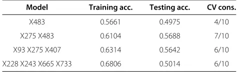
Table 9 MDR - Time duration: 15 minutes
Model Training acc. Testing acc. CV cons.
X483 0.5661 0.4975 4/10
X275 X483 0.6109 0.5561 6/10
X114 X216 X1070 0.6407 0.5937 9/10
X114 X315 X986 X1039 0.6844 0.5133 6/10
pair-wise distances. Without any loss of generality, we can thus project the large dataset into a lower dimensional space and can get the same result.
We have also employed PCA instead of random pro-jection in Algorithm 2 to compare the accuracy given by our techniques. The procedure is the same as described above. After applying FSA we pick the top 32 SNPs and apply PCA technique to find principal components of the feature space. The result is a list containing the coeffi-cients defining each component (sometimes referred to as loadings), the principal component scores, etc. We then compute the 1stprincipal component scores to 15th
prin-cipal component scores of each of the SNPs for each subject. After this data normalization and data discretiza-tion have been applied. FSA is then applied to the reduced dimensions of 10, and 15 respectively to classify the sub-jects of interest. The resulted maximum accuracy found was 73.685% [Please see Table 6]. Clearly, our random pro-jection method beats PCA in term of accuracy. Here again we see that random projections in conjunction with fea-ture selection are very effective in identifying statistically significant features of the input.
Algorithm 3
This approach validates the result of our feature selec-tion algorithm that it indeed gives more accurate results than another well known algorithm called multifactor dimensionality reduction or MDR. MDR has been used to identify potential interacting loci in several phenotypes. MDR is a SVM-like gene-selection classifier algorithm. We have compared our gene selection algorithm with MDR in terms of accuracy and runtime. This comparison reveals that our algorithm outperforms MDR with respect to the time to calculate the best number of SNPs that can together serve as a classifier. We ran MDR with the time intervals of 10 minutes, 20 minutes, 30 minutes, and 60 minutes. The SNPs identified by our algorithms form the
Table 10 MDR - Time duration: 30 minutes
Model Training acc. Testing acc. CV cons.
X483 0.5661 0.4975 4/10
X275 X483 0.6114 0.5555 5/10
X114 X216 X1070 0.6408 0.5810 8/10
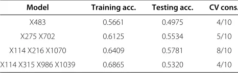
Table 11 MDR - Time duration: 60 minutes
Model Training acc. Testing acc. CV cons.
X483 0.5661 0.4975 4/10
X275 X702 0.6125 0.5534 5/10
X114 X216 X1070 0.6409 0.5781 8/10
X114 X315 X986 X1039 0.6865 0.5320 4/10
best subset of SNPs which are also given by MDR after running for 10 minutes and above whereas our FSA takes only 5 minutes to find the best SNPs with an accuracy of 73.805% [Please see Table 6] by employing linear SVM. But if we use polynomial kernel, FSA takes only 0.17 min-utes [Please see Table 6]. Here accuracy is the measure of how much confident we can be that the resulting SNPs can together serve as a classifier to distinguish two groups of subjects. Both programs were run on the same 2.8 GHz dual core machine.
Java implementation of MDR has been used for the anal-ysis of 1212 SNPs. There are three types of search methods available for driving the MDR, namely, exhaustive, forced and random. For each attribute count specified,
Exhaus-tive Method exhaustively examines each combination of
attributes. This search method has no options. Forced
Method examines only one attribute combination. The
combination must be specified in the provided text field as a comma-separated list of attribute labels. The labels are case-sensitive. And at last, for each attribute count specified, Random Method examines random combina-tions. There are two options here, namely, evaluations and runtime.Evaluation Optionevaluates a given number of random combinations, for each attribute count speci-fied. For each attribute count specified,Runtime Option
evaluates random combinations for a given amount of time. As theExhaustive Methodruns indefinitely for the pair-wise combination for the entire set of 1212 SNPs and the Forced Method is the totally irrelevant for our experiment, we used Random Method with the option ofRuntime.
The best single-locus model identified wasX483, with a training and testing accuracy of 56.61% and 49.75%, respectively but the cross-validation consistency was only 4 out of 10 after running for 5 minutes [Please see Table 7]. The best two-locus model identified wasX275, andX483, with a training and testing accuracy of 61.09% and 55.61%, respectively and cross-validation consistency was 6 out of 10 [Please see Table 8]. After running for 15 min-utes, MDR gave the best triple-locus model consisting of X114, X216, and X1070 with a training and testing accuracy of 64.07% and 59.37%, respectively [Please see Table 9]. The cross-validation consistency was 9 out of 10. On the contrary, our feature selection algorithm finds this combination after running for only 0.17 minutes with an
accuracy of 73.085% without employing any randomness [Please see Table 6]. The ternary-locus model identified after running for 30 minutes wasX114,X315,X986, and X1039 with a training and testing accuracy of 68.51% and 52.42%, respectively. The cross-validation consistency was 5 out of 10 [Please see Table 10]. After running for 60 minutes, MDR gave the best ternary-locus model consist-ing ofX114,X315,X986, andX1039 with a training and testing accuracy of 68.65%, and 53.20%, respectively. But the cross-validation consistency was of only 4 out of 10 [Please see Table 11].
Conclusions
A subset of single nucleotide polymorphisms (SNPs) can be used to capture the majority of the information of genotype-phenotype association studies. The primary purpose of this research is to select a subset of SNPs while maximizing the power of detecting a significant associa-tion. From this point of view, we have proposed a number of approaches to find a subset of SNPs from the entire set to classify a set of individuals. Our proposed algo-rithms are indeed efficient, reliable, and scalable in terms of both accuracy and time complexity. Random projection has been used to project the data onto a lower dimensional space. A subset of attributes is then selected from this low dimensional space. To the best of our knowledge, ran-dom projection technique has not been employed before in the area of SNPs analysis. As revealed by our experi-mental results, these techniques offer the potential of high accuracies while keeping the run times low.
Competing interests
All authors declare that they have no competing interests.
Authors’ contributions
SS contributed to the implementation of the algorithms, testing and analysis, manuscript preparation, algorithms development, and performance analysis. SR contributed to algorithms development, analysis of the results, performance analysis, and manuscript preparation. JB contributed to data preparation, results analysis, and performance analysis. SP contributed to the implementation of the algorithms. All the authors have read and approved the final manuscript.
Acknowledgements
This research has been supported in part by the NSF Grant 0829916 and the NIH Grant R01-LM010101.
Received: 14 February 2013 Accepted: 19 March 2013 Published: 4 April 2013
References
1. Single-nucleotide Polymorphism.[http://en.wikipedia.org/wiki/Single_ nucleotide_polymorphism]
2. Cooper DN, Smith BA, Cooke HJ, Niemann S, Schmidtke J:An estimate of unique DNA sequence heterozygosity in the human genome.Hum Genet1985,69:201–205.
3. Collins FS, Guyer MS, Charkravarti A:Variations on a theme: cataloging human DNA sequence variation.Science1997,278:1580–1581. 4. Song M, Rajasekaran S:A greedy correlation-incorporated SVM-based
5. Achlioptas D:Database-friendly random projections:
Johnson-Lindenstrauss with binary coins.J Comput Syst Sci2003, 66(4):671–687.
6. Ritchie MD, Hahn LW, Roodi N, Bailey LR, Dupont WD, Parl F, Moore JH: Multifactor-dimensionality reduction reveals high-order
interactions among estrogen-metabolism genes in sporadic breast cancer.Genet2001,69:138–147.
7. Tabor HK, Risch NJ, Myers RM:Candidate-gene approaches for studying complex genetic traits: practical considerations.Nat Rev Genet2002,3(5):391–397.
8. Hodgkinson etal:Addictions biology: haplotype-based analysis for 130 candidate genes on a single array.Alcohol Alcohol2008, 43(5):505–515.
9. Saeys Y, et al:A review of feature selection techniques in bioinformatics .Bioinformatics2007,23(19):2507–2517. doi:10.1093/bioinformatics/btm344.
10. Mitchell T:Machine Learning.New York: McGraw Hill; 1997. 11. Waddell M, Page D, Zhang F, Barlogie B:Predicting cancer
susceptibility from single-nucleotide polymorphism data: A case study in multiple Myeloma.Chicago: BIOKDD; 2005.
12. Goertzel BN, Pennachin C, Coelho LS, Gurbaxani B, Maloney EM, Jones JF: Combination of single nucleotide polymorphisms in
neuroendocrine effector and receptor genes predict chronic fatigue syndrome.Pharmacogenomics2006,7:475–483.
13. Listgarten J, Damaraju S, Poulin B etal:Predictive models for breast cancer susceptibility from multiple single nucleotide
polymorphisms.Clin Cancer Res2004,10:2725–2737.
14. Üsünkar G, Özögür-Akyüz S, Weber GW, Friedrich CM, Son YA:Selection of representative SNP Sets for genome-wide association studies: A metaheuristic approach.Optimization Lett2012,6(6):1207–1218. doi:10.1007/s11590 ˝U011-0419 ˝U7.
15. Meng Z, Zaykin DV, Xu CF, Wagner M, Ehm MG:Selection of genetic markers for association analyses, using linkage disequilibrium and haplotypes.Am J Hum Genet2003,73:115–130.
16. Horne B, Camp NJ:Principal component analysis for selection of optimal SNP-sets that capture intragenic genetic variation.Genet Epidemiol2004,26:11–21.
17. Vapnik VN:The Nature of Statistical Learning Theory.Berlin: Springer-Verlag; 1995.
18. Cortes C, Vapnik V:Support vector networks.Mach Learn1995,20:1–25. 19. Lee Y, Lin Y, Wahba G:Multicategory support vector machines,
theory, and application to the classification of microarray data and satellite radiance data.J Amer Stat Assoc2004,99(465):67–81. 20. Joachims T:Transductive inference for text classification using
support vector machines.InProceedings of the 16thInternational
Conference on Machine Learning (ICML). San Francisco: Morgan Kaufmann Publishers Inc; 1999:200–209. ISBN 1-55860-612-2.
21. Hsu CW, Lin CJ:A comparison of methods for multiclass support vector machines.IEEE Trans Neural Netw2002,13(2):415–425. 22. John and Stephens, M:Interpreting principal component analyses of
spatial population genetic variation.Nat Genet2008,40:646–649. doi:10.1038/ng.139.
23. Boas and Mary, L:Mathematical Methods in the Physical Sciences. 2nd edn. New York: Wiley; 1983.
24. Abdi H, Williams LJ:Principal component analysis.Comput Stat, Wiley Interdisciplinary Rev2010,2:433–459.
25. Isabelle G, Weston J, Barnhill S, Vapnik VN:Gene selection for cancer classification using support vector machines.Mach Learn2002, 46:389–422.
26. LeCun Y, Denker JS, Solla SA:Advances in Neural Information Processing Systems 2.Edited by Touretzky, Morgan, Kaufmann; 1990:598–605.
27. Johnson WB, Lindenstrauss J:Extensions of lipschitz mappings into a Hilbert space.InConference in Modern Analysis and Probability; 1984:189–206. Providence: Amer. Math. Soc.
28. Ritchie MD, Hahn LW, Moore JH:Power of multifactor dimensionality reduction for detecting gene - gene interactions in the presence of genotyping error, missing data, phenocopy, and genetic heterogeneity.Genet Epidemiol2003,24:150–157.
29. Ritchie MD, Hahn LW, Moore JH:Multifactor dimensionality reduction software for detecting gene - gene and gene - environment interactions.Bioinformatics2003,19:376–382.
30. Martin ER, Ritchie MD, Hahn L, Kang S, Moore JH:A novel method to identify gene-gene effects in nuclear families: the MDR-PDT.Genet Epidemiol2006,30:111–123.
31. Coffey CS, Hebert PR, Ritchie M D,et al:An application of conditional logistic regression and multifactor dimensionality reduction for detecting gene - gene interactions on risk of myocardial infarction: The importance of model validation.BMC Bioinformatics2004,5:49.
doi:10.1186/1472-6947-13-41
Cite this article as:Sahaet al.:Efficient techniques for genotype-phenotype correlational analysis.BMC Medical Informatics and Decision Making 2013 13:41.
Submit your next manuscript to BioMed Central and take full advantage of:
• Convenient online submission
• Thorough peer review
• No space constraints or color figure charges
• Immediate publication on acceptance
• Inclusion in PubMed, CAS, Scopus and Google Scholar
• Research which is freely available for redistribution