Delay Efficient Backpressure Routing in Wireless
Ad Hoc Networks
H
Leandros A. Maglaras
1, Dimitrios Katsaros
1,∗1University of Thessaly, Department of Electrical & Computer Enginnering, 382 21 Volos, Greece
Abstract
Packet scheduling/routing in wireless ad hoc networks is a fundamental problem for ad hoc networking. Backpressure routing is a solid and throughput optimal policy for such networks, but suffers from increased delays. In this article, we present two holistic approaches to improve upon the delay problems of backpressure-type algorithms. We develop two scheduling algorithms, namely Voting backpressure and Layered backpressure routing, which are throughput optimal. We experimentally compare the proposed algorithms against state-of-the-art delay-aware backpressure algorithms, which provide optimal throughput, for different payloads and network topologies, both for static and mobile networks. The experimental evaluation of the proposed delay reduction algorithms attest their superiority in terms of QoS, robustness, low computational complexity and simplicity.
Keywords: Packet scheduling/routing, Delay Reduction, Ad Hoc Networks, Mobile networks
1. Introduction
Wireless ad hoc (multi-hop) networks lack fixed infras-tructure (e.g., base stations, mobile switching centers). The communication between any two nodes that are out of one another’s transmission range is achieved through intermediate nodes. These intermediate nodes relay messages to set up a communication channel. Contemporary application areas of the ad hoc networks include modern battlefields, disaster relief, precision agriculture, e-health, ocean monitoring with underwater wireless sensor networks. Packet transmission scheduling in this type of networks is a fundamental issue since it is directly related to the achievement of a prescribed Quality of Service (QoS) and a minimum use of system resources. QoS is usually measured in terms of the average packet delay, transmission rate and maximum delay, and the main system resource to be saved is the nodes’ energy so as to prolong network lifetime. In addition to delay and energy optimization, any packet scheduling/routing algorithm for ad hoc networks must be resilient to topology changes and strive for throughput optimality.
The development of a throughput-optimal routing algorithm for packet radio networks which is also robust to topology changes was first presented in [2]. It is based on the Lyapunov drift theory, and it is known as the backpressure (BP) packet scheduling algorithm.
HThis is an extended version of the paper [1]
∗Corresponding author. Email:[email protected]
Subsequently, the original concept spawns several lines of research on the topic. The performance of backpressure deteriorates in conditions of low, and even of moderate, load in the network, since the packets “circulate” in the network, i.e., the backpressure algorithm stabilizes the system using all possible paths throughout the network. The negative effect of this algorithm is to increase delay and also to increase the energy consumption of the nodes that play the role of relays. End to end delay and energy consumption are interconnected. The minimization of the average time that the packets stay in the system, implies a reduction in the average number of hops that the packets travel until they reach their destination, which in turn implies a reduction in the total energy consumption. Delay and energy consumption problems are particularly significant for ad hoc sensor networks. Routing-loop formation is another drawback of backpressure routing. In many real time applications like voice and video, high end-to-end packet delay is unacceptable. Often in such applications, a packet received with a high delay is not better than packet loss. High end-to-end delay can be prevented by not forwarding the packets on longer paths. On the other hand, in order to provide adequate load balancing in case of high traffic load, sufficient routes need to be maintained for any source-destination pair. Generally, these two objectives conflict with each other because few short routes exist in the network.
Tocircumventthedelayproblemofbackpressure,the mean resource routing algorithm [3] forces the links to
Research
Article
EAI Endorsed Transactions
on
Mobile
Communications
and
Applications
Receivedon 02 April 2014;acceptedon29 August 2014;publishedon24 September 2014
Copyright©2014 Leandros A, Maglaras and Dimitrios Katsaros, licensedtoICST.Thisisanopenaccessarticledistributed under the terms of the Creative Commons Attribution license (http://creativecommons.org/licenses/by/3.0/), whichpermitsunlimiteduse,distributionandreproductioninanymediumsolongastheoriginalworkisproperlycited.
L.Maglaras and D.Katsaros
stay inactive in order to lead the network to work in a burst mode, since for periods when the load of the network is low or moderate, link activation is prevented by a parameter M, leading to a delay increase. On the other hand, the relatively high computational cost incurred at each node by backpressure (maintenance of a queue for each possible destination, and update of these queues at each new arrival) inspired approaches based onnode groupingin order to reduce the number of these queues [4] and thus the computational overhead, and as a side-product, reduce the delay. To alleviate the delay problems of backpressure, scheduling based on the combination of backpressure and shortest-paths have been proposed [5], which though demands an excessive number of queues and repeated calculation of all-node-pairs distances in case of topology changes. In summary, all these approaches either impose unpractical and non scalable assumptions, or are not very efficient. Finally, some recent ideas [6, 7] could be incorporated in an orthogonal way to improve analogously the delay performance of all policies, but this is beyond the scope of this paper. Here, we take holistic approaches in designing efficient delay-aware backpressure algorithms, which are both practical – have low computational overhead and are robust to topology changes.
1.1. Motivation
In the mean resource routing (MR−BP) algorithms [3,
8], backpressure is used with a parameterM that forces the links to stay inactive as long as their differential backlog does not exceed the value ofM, i.e., links with backpressure less than M cannot be scheduled. This means that packets stay in queues longer, which can lead to higher delays. Indeed, we tested this intuitive result in [1] by evaluating the delay performance of these algorithms and confirmed this behavior. Therefore, since theMR−BP algorithms are not delay competitive, we do not consider them as viable competitors any more.
The authors of [4] identified the scalability problems of the backpressure algorithm inwireline networks with millions of routers (e.g., Internet) due to the maintenance of several queues per node (one queue per destination, as it is mandated by the original BP), and proposed the creation of clusters1 of nodes so as to reduce the number of queues per node, which as a “side-product” has the additional benefit of delay reduction. Their algorithm, namely cluster-based backpressure(CB−BP), requires maintaining one queue per gateway at each relay node, leading to an excessive number of gateways, which in turn alleviates any performance gains (i.e., increases delays) when the number of clusters becomes, say, more than ten. Even worse, all contemporary clustering algorithms [9, 10] (such as the Distributed
1The authors did not propose any specific clustering algorithm.
Clustering algorithm and the Max-min d-hop clustering algorithm) for wireless ad hoc networks produce quite a large number of clusters and thus several dozens of gateways even for relatively small networks. In these cases, the delays of CB−BP algorithms asymptotically reach the delays of the original BP (cf. Figure 6c). Moreover, the strong dependence of the policy on the identity of the gateways makes it problematic in cases of gateways breakdowns. Finally, considering the technicalities of theCB−BP algorithm, it is evident that even when a packet has already reached the destination cluster (i.e., the cluster where the destination nodes resides), the algorithm is agnostic on this information and it may happen to send it again out of the cluster seeking alternative paths to the destination. This behavior is detected and improved in our experiments (cf. subsection6.1).
The Shortest-paths backpressure (SP−BP) algo-rithm [5] assumes the pre - computation of all pairwise-node distances and then application of the backpressure notion on the shortest path(s) between source and des-tination. Apparently, this algorithm achieves the lower bound of the delay. It does so at the expense of a very complex initialization phase (all-node-pairs dis-tances must be computed). Moreover, it must maintain a quadratic number of queues at each node [n×(n−1)], whereas the original backpressure maintains only a linear number of queues (n−1) at each node. Also, during the running phase of the algorithm, the processing of such a huge number of queues is time-consuming, which in turn increases delays. Apart from these computational-type problems, frequent topology changes leads the algorithm to break down, since many shortest paths do not exist anymore. Finally, in the topologies where there is only one shortest-path per node pair (which is the most common case), SP−BP rapidly consumes the energy of that path, shortening the longevity of the network. This problem becomes worse in the topologies where a lot of shortest paths traverse the same set of nodes (i.e., the nodes with high betweenness centrality [11]). In such topologies, these nodes deplete their energy so fast that the network gets partitioned very rapidly.
1.2. Contributions
The present article develops two scheduling algorithms, namely the Voting-based Backpressure (VoBP) and the Layered Backpressure (LayBP).
create “layers” of nodes and use the identities of these layers to forward the packets toward the destination’s layer, and “discouraging” the packets from leaving the destination layer; these layers act as attractors for the packets.
The two proposed algorithms aim to decrease the mean end to end delay of the packets while mainting throughput performance optimal. LayBP, which is a global-network-topology-aware algorithmg, splits the network in small subnetworks and guides the packets towards their destination subnetwork, without forcing them to follow specific routes. This procedure can significantly improve the performance of a routing algorithm in terms of mean delay, and it can be used in a any topology regardless of shape and size. On the other hand information about the traffic in a local aspect is exploited byVoBP. The proposed algorithm dynamically adapts the routing of packets locally, according to the current situation of the network. LayBP is a static method that is based on the split of the network in smaller parts while VoBP is a dynamic algorithm that routes packets according to their travel history. The two proposed algorithms exploit different characteristics of the network (topology vs traffic) in order to decrease the end to end delay of packets. Moreover LayBP is global-network-topology-aware algorithm whileVoBP is a local-network-topology-aware one. The two proposed algorithms may be combined in order to further improve the performance of the system.
The article makes the following contributions:
• It experimentally evaluates well established delay-aware backpressure policies, namely BP, MR−BP, CB−BP, SP−BP for several network topologies.
• It develops the Voting-based Backpressure pol-icy, which “wipes-outs” the ping-pong effect in backpressure-based packet scheduling. The algo-rithm exploits current traffic in the network in order to lead packets away from already visited nodes, vanishing rooting-loop.
• It develops the Layered BackPressure (LayBP), which divides the network into “layers” according to the connectivity of nodes. This algorithm maintains the same number of queues with the original BP, and one order of magnitude less number of queues compared to SP−BP. It does not require the existence of gateways and aggregated queues as does CB−BP. In complex networks gateways may be so many that CB−BP performs like original BP. In addition, it is not a deterministic algorithm like SP−BP where packets are forced to travel the shortest-path among nodes. Instead the packets are “suggested”
to follow the shortest path from the source to the destination layer.
• It develops the Enhanced Layered Backpressure policy EL−BP that improves the behavior of LayBP in case of moving nodes. The new algorithm have the same characteristics with the LayBPand is robust to topology changes in terms of nodes that move from one layer to another.
• It develops a new random-walk based node clustering algorithm, that exploits the connectivity among nodes.
• It evaluates experimentally the performance of the proposed packet scheduling policies, with all the previous delay-aware throughput optimal backpressure algorithms.
The rest of this article is organized as follows: Section2
describes the network model; Section 3 introduces the original backpressure scheme; Section 4 presents the VoBP scheme; Section 5 describes the LayBP algorithm; Section5.4describes theEL−BP algorithm; Section 6 presents the simulation environment and results; Section 7 reviews the most important works relevant to this article, and finally Section 8 concludes the article.
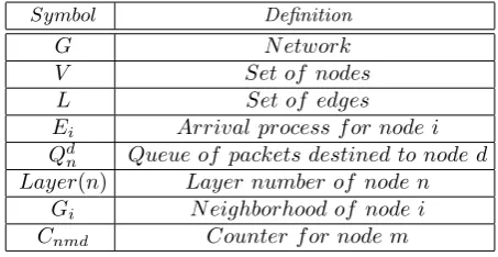
Table 1 summarizes the basic notations used in the article.
Symbol Definition
G N etwork
V Set of nodes
L Set of edges
Ei Arrival process f or node i
Qd
n Queue of packets destined to node d
Layer(n) Layer number of node n Gi N eighborhood of node i
Cnmd Counter f or node m
Table 1. Notation table
2. Network model
We consider a network G= (V, L), where V is the set of nodes (vertices) andL is the set of links (edges). We consider the following generic properties:
• Nodes are static or mobile, the communication links are bidirectional, and nodes communicate in a multi-hop fashion.
L.Maglaras and D.Katsaros
• Network nodes are homogeneous and do not have GPS-like hardware. Links have equal to one capacity.
• Concurrent transmissions cause mutual interfer-ence since the transmission medium is shared. Matchings are the set of links that can be scheduled simultaneously. A max-weight scheduling policy is used.
• A node cannot transmit and receive at the same time.
• Time is slotted with a time slott.
• For each node i, there is an arrival process Ei
such that Ei(t) is the number of exogenous
arrivals up to time t. We assume that packets arrive exponentially with mean arrival rateλ. The source and destination of each packet is randomly selected among all the nodes. Special cases are also investigated by using the Zipf’s distribution, where packets ’prefer’ some nodes as destinations representing a more realistic scenario.
3. The original Backpressure algorithm
Backpressure [2] is a joint scheduling and routing policy which favors traffic with high backlog differentials. The backpressure algorithm performs the following actions for routing and scheduling decisions in every time slott.
• Resource allocation
For each link (n, m) assign a temporary weight according to the differential backlog of every commodity (destination) in the network:
wtnmd(t) =max(Qdn−Q d m,0).
Then, define the maximum difference of queue backlogs according to:
wnm(t) = max
dD wtnm(t).
Let d∗mn[t] be the commodity with maximum backpressure for link (n,m) in time slott.
• Scheduling
The network controller chooses the control action that solves the following optimization problem:
µ∗(t) =argmax
µΓ
X
(n,m)L
µnmwnm(t),
, where Γ denotes the set of all schedules subject to the one hop interference model.
In our model, where the capacity of every linkµnm
equals to one, the chosen schedule maximizes the sum of weights. Ties are broken arbitrarily.
• Routing
In time slott, each link (n, m) that belongs to the selected scheduling policy forwards one packet of the commodityd∗mn[t] from nodento nodem. The routes are determined on the basis of differential queue backlog providing adaptivity of the method to congestion.
The backpressure algorithm is throughput-optimal and discourages transmitting to congested nodes, utilizing all possible paths between source and destination. This property leads to unnecessary end-to-end delay when the traffic load is light. Moreover, using longer paths in cases of light or moderate traffic wastes network resources (node energy).
4. Voting-based backpressure
The driving idea behind theVoBPscheduling algorithm is the reduction of the path length traveled by a packet by reducing any cycles observed on this path. Apparently, this can be done by having the packet ”carrying” its trajectory. Such an approach though, would comprise the properties of the backpressure algorithm (i.e., utilize all paths), and also it would be impractical, since these trajectories grow remarkably large for long paths, having as a consequence a considerable increase in the packet size and increased processing time by the routers. Therefore the storage of such “rich” information in the packets is not a viable option, unless we confine the amount of information. This is exactly the direction followed by theVoBP algorithm.
VoBPuses minimum information stored in the packets in order to select the scheduling policy in each time slot. Every packet holds the last node it has previously visited. This information is used in the scheduling phase of the algorithm in order to prevent packets from revisiting the same nodes and traveling in circles in the network. Each node n maintains a separate queue of packets for each destination Qd
n[t] (as the original backpressure
algorithm). Each queuedhas a counter for each neighbor nodeCnmd. This counter is updated every time a packet
arrives to or leaves from node n having as destination node d. Since the packet holds the information about the last visited node a certain procedure is followed at each transition.
When packet i having as final destination node d arrives at nodenfrom nodemthe following actions take place.
• At noden Cnmd is incremented by one.
• At nodem Cnmd is decremented by one.
• Packetiupdates last visited node frommton.
updating the appropriate counters. A vote is given according to Definition1.
Definition 1 (Vote).A packet (destined to node d) that arrives to node n assigns a vote to node m it has previously visited. This vote is represented by incrementing counterCnmd by one.
The votes are positive counters but have the meaning of negativity. The neighboring node with the most votes is the worst candidate for routing packets towards it. Based on the information of the packets, the scheduling algorithm assigns an appropriate weight to the corresponding links, preventing this way the controller from choosing such a routing policy that moves the packets backwards in the network. Parameter A is used in order to assign weights to links and help the routing mechanism forward packets to delay efficient paths. The tuning of this parameter is evaluated in section 6.1. The Voting-based backpressure algorithm executes in time slott as follows:
• Each queue votes for the Bad neighbor Bnmd of
node naccording to:Bnmd = maxCnmd.
• Each link (m, n) is assigned temporary weights according to the differential backlog wtnmd(t) =
max(Qdn−Qdm,0) and a parameter Anmd
accord-ing to :
Anmd=
1/A, ifm=Bnmd
1 otherwise.
• Each link is assigned a final weight according to wnm and parameterAnmd:
wnm(t) = max
dD(wtnmd(t)∗Anmd).
• The network controller chooses the control action that solves the following optimization:
µ∗(t) =argmax
µΓ
X
(n,m)L
µnmwnm(t)
subject to the interference model mentioned above where adjacent links are not allowed to be active simultaneously.
In each time slot only nodes that transmit or receive packets update the information in the appropriate queues decreasing the complexity of the algorithm. Except from the worst node, also the good node Gnmd (Gnmd=
minCnmd) or the nodes to send packets can be retrieved
from the above procedure giving an extra bonus to this node for the corresponding queue. Good nodes should be the ones with the least or even zero votes, meaning that no packet has visited them in the previous hop.
ParameterAnmd would be in that way:
Anmd=
A, ifm=Gnmd
1/A, ifm=Bnmd
1 otherwise.
As shown in the experiments (cf. subsection 6.1), this algorithm can significantly reduce delays in low-loaded wireless networks, and moreover, it can be used in combination with other backpressure-type algorithms to enhance their performance. The algorithm shows extremely good performance in networks with very low connectivity between nodes where only a few paths exist for the packets to follow in order to reach their destinations. The packets by holding the information about the previously visited nodes help the fast propagation of the information.
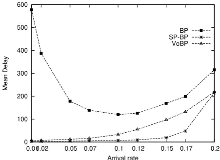
Even though a detailed evaluation of the algorithm is presented in a later section, to support the above claims we tested the algorithm in a ring network consisting of twelve nodes (see Figure 1). The performance of VoBP is similar to that of the shortest path backpressure. This performance is achieved without the need of any extra queues or other information, like all the distances among the nodes, except from the last visited node that every packet holds.
0 100 200 300 400 500 600
0.01 0.02 0.05 0.07 0.1 0.12 0.15 0.17 0.2
Mean Delay
Arrival rate
BP SP-BP VoBP
Figure 1. Performance of VoBP in a 12-node ring network
5. Layered backpressure
This section describes a delay-efficient backpressure algorithm based on the creation oflayers2in the network. The main idea is to split the network into layers according to the connectivity among them, which also
L. Maglaras, D. Katsaros
(usually) implies geographic proximity, as well. These layers divide the initial graph to k smaller networks. Then the algorithm forwards packets according to the destination layer ID, thus effectively reducing the long paths. In some sense, these layers play the role of attractors, which attract the packets destined for them and then “disallow” the packets to leave the layer. Apparently, if we have only one layer, the algorithm reduces to the original backpressure algorithm.
For the implementation of the LayBP scheduling policy, every node n keeps a separate queue for each destination/flow going through it and also holds the layer Layer(n) that the destination belongs to. The backpressure scheduling is executed using only the IDs of these layers. This is a significant difference from the work of [4], becauseLayBPdoes not require the knowledge of gateways’ queue lengths. The “correct” partitioning of nodes into layers and a proximity-based naming of layers is of paramount importance for the performance of every routing algorithm which based on clustering. Since in the proposedLayBPalgorithm no gateways are required the algorithm is more robust to bad partitioning. Also the algorithm, as it is shown in section 6.1, performs better as the number of clusters grow, in contrast to CB−BP. Apparently, the concept of ”correctness” is algorithmic, and we only need to set a partitioning criterion. Therefore we propose to determine the number of layers based on the network topology, i.e., connectivity. The next two subsections describe the layer-creation and layer-naming algorithm, whereas subsection5.3presents the Layered Backpressure packet scheduling algorithm.
5.1. Random-walk-based layering
In this section, we present a random walk based clustering (RW C) method for creating the necessary layers.RW Cruns in the initiation phase of the network. The method is centralized and the number of layersN cto be created are discovered by an exhaustive cost-optimal algorithm. Techniques for estimating this number can be found at [11]. The layers created by this algorithm have approximately the same cardinality, which is denoted by the parameter N pc. Every node has a parameter indicating if the layer it belongs to is “final” or not. At the beginning of the algorithm all nodes are assigned a random layer ID, from 1 to N c. The final layer of each node is determined by the RWC algorithm after a number of iterations. For all the nodes that do not have their layers fixed by the algorithm yet, we say that they belong to a “temporary” layer.
The algorithm runs in blocks where in each block a node i is selected as a source. The algorithm takes successive random steps from ifor a predefined number of steps hforK iterations. Every node holds a counter indicating how many times it is visited from the random
walk algorithm in the current block. The neighborhood of the nodeiis created according to Definition 2.
Definition 2 (Neighborhood of node i).A nodejbelongs to the neighborhood Giof the node i, if the number of times the node is visited is at least equal to the times the RWC traversed node i.
After the creation of the neighborhood Gi the proposed algorithm operates as follows:
1. Find the layer P oslevel having the maximum number of members of the current neighborhood. This is the possible layer of all the nodes that belong to theGi.
2. If this layer is different from the layer of source nodei then find a node outside the neighborhood that has this temporary layer and exchange values (layers) with nodei.
3. If the number of members of the P oslevel is less thanN pcand greater than one then try to find a node outside the layer with this temporary layer and exchange layers with a node belonging to theGnibut having temporary layer different from theposLevel.
4. If the number of nodes that belong to the possible level after the previous steps isN pcwith deviation of one then the layer of these nodes is fixed to theP oslevel.
The procedure moves in small steps inserting at each iteration at most two nodes in the possible layer leading to a relatively fair clustering of the nodes after its termination. This procedure is repeated for each node belonging to a temporary layer until all the layers are fixed. The nodes that after this procedure still belong to temporary layers fix their values according to the layers of their neighbors.
5.2. Naming of Layers
5.3. The Layered BackPressure algorithm
After the completion of the grouping and the assignment of IDs to the layers, the actual packet scheduling is performed as follows. Each node nmaintains a separate queue of packets for each destination. The length of such a queue is denoted byQd
n(t). For every queueQdn(t) the
node computes the parameterDleveld
n which represents
the absolute difference between current and destination nodes’ layer number:Dleveld
n =|Layer(n)−Layer(d)|.
In each time slot t, the network controller observes the queue backlog matrix Q(t) = (Qdn(t)) and performs the
following actions for routing:
Layered BackPressure in time slott:
• Each link (n,m) is assigned a temporary weight according to the differential backlog wtnmd(t) =
(Qd
n−Qdm) and parameterAnmd according to:
Anmd=
2, ifDleveld
n > Dleveldm
1/2, ifDlevelnd < Dleveldm
1 otherwise.
• Each link is assigned a final weight according to wnm and parameterAmnd:
wnm(t) = max
dD(wtnmd(t)∗Anmd).
• The network controller chooses the control action that solves the following optimization:
µ∗(t) =argmax
µΓ
X
(n,m)L
µnmwnm(t)
subject to the interference model mentioned above where adjacent links are not allowed to be active simultaneously.
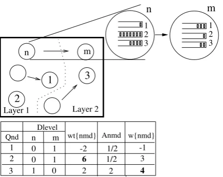
A simple example is illustrated in Figure 2. The network consists of7nodes where all nodes are senders and only nodes with id’s1,2,3are destination nodes. We observe the status of the queue backlogs in a specific time slot t. The network is divided in two layers. Layer one includes nodes on the left side of the dot line. Running the initial backpressure algorithm the commodity that achieves maximum differential backlog for link (n, m) is 2 while for the proposed layered backpressure is 3. If we assume that link (n, m) is scheduled in that time slot then for the initial backpressure algorithm a packet destined for node2will be forwarded to nodempushing it further away and forcing it to follow a longer path in order to reach its destination (node 2). With the layered backpressure policy at the same time link (n, m) if scheduled forwards a packet of commodity 3 from node n to node m which is closer to the destination of the packet. Furthermore, node m belongs to the same cluster as node n, which according to the proposed
2
Qnd
Dlevel
w{nmd} wt{nmd}
1/2 2 1/2
0 3
Layer 2
BP : Optimal commodity for link (n,m) on slot t is 2. w(n,m) = 6 3 1
LBP : Optimal commodity for link (n,m) on slot t is 3. w(n,m) = 4 6
4 -1 3 -2
2 1 0 0 1
1 m n 1 2 Layer 1
2 1
3
3
1
2
Anmd m n
n
m
Figure 2. An example of theLayBP execution.
layer backpressure policy will prevent the packet from returning to noden.
Theorem 1 (Throughput optimality).The LayBP and VoBP algorithms are throughput optimal.
Lemma1 is useful for the proof of the theorem.
Lemma 1. IfV, U, µ, A are nonnegative real numbers andV ≤max[U−,0] +Athen
V2≤U2+µ2+A2−2U(µ−A)
Proof. The original backpressure algorithm is through-put optimal. In order to prove that the VoBP and LayBP are also throughput optimal, the Lyapunov stability criterion is used. The idea behind the Lyapunov drift technique is to define a non-negative function, called the Lyapunov function, which represents the aggregate congestion of all queues (Qd
n) in the network. The drift
of the function in two successive time slots is then taken, and in order for the policy to be throughput optimal, this drift must be negative, when the sum of queue backlogs is sufficiently large. For both policies, we use:
L(Q) =X
nd
θnd(Qdn)2 (1.1)
as the Lyapunov function where weights θd
n are used to
offer priority service.
Recall that each link is assigned a final weight according townm and parameterAmnd:
L.Maglaras and D.Katsaros
The Equation 1.2 can be rewritten in the following form:
wnm(t) = max
dD(Anmd∗Q d
n−Anmd∗Qdm). (1.3)
which is equivalent to :
wnm(t) = max dD(θ
d n∗Q
d n−θ
d m∗Q
d
m), (1.4)
where weightsθd
i are used to offer priority service similar
to [13].
Queue dynamics in each time slot satisfy :
Qdn(t+ 1)≤max[Qdn(t)−X
b
µdnb(t),0]+
Adn(t)−X
a
µdan(t)
(1.5)
,whereµd
nm(t) are routing control variables, representing
the amount of commodity d data delivered over link (n, m) during slott and Ad
n(t) represent the process of
exogenous commodityddata arriving to source node n. P
bµ d
nb(t) represents the total amount of commodity
ddelivered over all outgoing links of noden. We assume that only the data Qd
n(t) currently in node n at the
beginning of slot t can be transmitted during that slot. The above expression is an inequality rather than an equality because the actual amount of commodity d data arriving to node n during slott may be less than P
aµ d
an(t) if the neighboring nodes have little or no
commodityddata to transmit.
We apply Lemma 1 to the queuing equation 1.5 and obtain:
(Qdn(t+ 1))2≤([Qdn(t))2+ (X
b
µdnb(t))2+ (Adn(t)+
X
a
µdan(t))2−2[Qdn(t)(X
b
µdnb(t)−Adn(t)−µdan(t))
(1.6)
Multiplying both sides withθd
n, summing over all valid
entries (n, d) and using the fact that the sum of squares of non-negative variables is less than or equal to the square of the sum we take :
X
nd
θnd(Qdn(t+ 1))2≤
X
nd
θdn(Qdn(t))2+
X
nd
θnd(X
b
µdnb(t))2+X
nd
θdn(Adn(t) +X
a
µdan(t))2
−2X
nd
θdnQdn(t)(X
b
µdnb(t)−Adn(t)−µdan(t)) (1.7)
The equation can be rewritten:
∆L(Q)≤2BN−2X
nd
θdnQdn(t) (1.8)
,where
B , 1 2N
X
nεN
θmax[(µoutmax,n)
2+ (Amax n +µ
in max,n)
2]
(1.9) Using the above we can rewrite drift inequality :
∆L(Q)≤2B0N θmax−2
X
nd
θdnQdn(t) (1.10)
,where
B0, 1 2N2
X
nεN
[(µoutmax,n)2+ (Anmax+µinmax,n)2] (1.11)
This drift inequality is in the exact form for application of the Lyapunov drift lemma, proving the stability of the algorithm.
The weighted sum of all queues is :
lim sup t→∞ 1 t t X τ=0 E{X
n,d
θndQdn(τ)} ≤ N B 0θ
max
max
(1.12)
InVoBPalgorithm where the weights are dynamically varying over time, such that θd
n∈[θmin, θmax], network
stability is still ensured [13].
5.4. The Enhanced Layered Backpressure policy
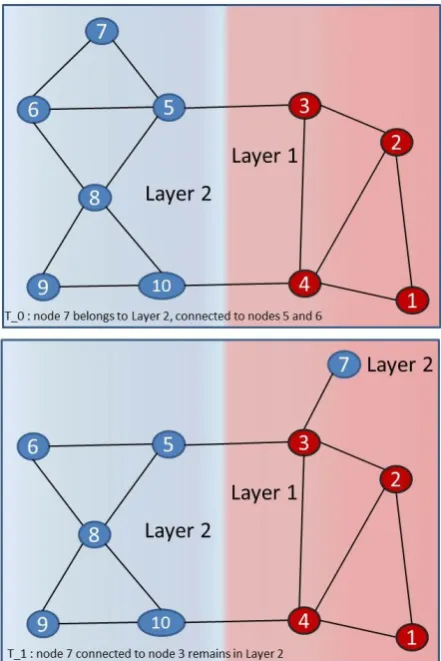
Looking at Figure3we see that node7(moving node) initially belongs to cluster2at momentT0. At moment T1 node7moved to cluster 1but is agnostic of it. The packets destined to node 7 are still forwarded by the LayBPto cluster2making it difficult to reach their final destination thus making the intermediate node’s queues to grow up.
Figure 3. Example network with a moving node.
In order to cope with node mobility we incorporate in the LayBP algorithm another step. Both moving and static nodes use this additional step in order to recalculate their cluster according to their neighborhood. In the initiation phase every node has a counterC0n,lfor
every layer ID, indicating how many neighbors belong to it and a variable Layern indicating the layer that node
n belongs to. In every time slot t the following actions are performed:
• Calculate Cn,l, the total number of neighbors that
belong to every layer detected.
• if Cn,l>=C0n,l for l=Layern then the moving
node remains in the same layer.
• else calculate the layer with the most neighbors Mn,l=maxCn,l. if Mn,l> Cn,l then the moving
node belongs to layerMn,l.
• assign for every layerl,C0n,l=Cn,las new initial
values for the next time slot.
This procedure can be executed every k time slots according to how fast we want the system to adapt to node mobility. The moving nodes need to execute the procedure every second in order to find the appropriate layer they belong to. The static nodes need to update their information more rarely, than the moving nodes do, since a certain number of neighbors must be replaced in order to affect them. The procedure does not perform reclustering, but only ‘helps’ layers incorporate moving nodes.
6. Evaluation
For the evaluation of the proposed scheduling policies we developed a custom simulator, modeling topology features, packet scheduling, link activation, etc. We consider as competitors the state-of-the-art delay-aware backpressure policies that have been published so far in the literature, with the exception of the MR−BP policies which were shown in subsection1.1to provide no delay performance benefits. We simulate the execution of the algorithms for various network topologies for large simulation times and recorded their average performance. In the interest of space, we show only the most representative results.
6.1. Static networks
Experimental setting. As of competing algorithms we examine currently proposed delay-aware backpressure algorithms along with the original backpressure algo-rithm as the baseline algoalgo-rithm. We emphasize here that the shortest path backpressure [5] is theoretically optimal w.r.t. delay. This algorithm performs the best in all cases and acts as the lower bound, but it is vulnerable to topol-ogy changes (cf. Figure10). For the algorithms needing some form of clustering, i.e., CB−BP and LayBP, the clustering is performed with the proposed random-walk clustering algorithm. For theCB−BP in order to improve the misbehavior of the algorithm when the source and destination are in the same cluster, the traffic controller can directly route them without relaying to any gateway, even if source is a gateway ofcluster(d) itself.
Performance metrics. As performance measures we
use the average end-to-end delay and the number of messages successfully delivered per unit time (network throughput).
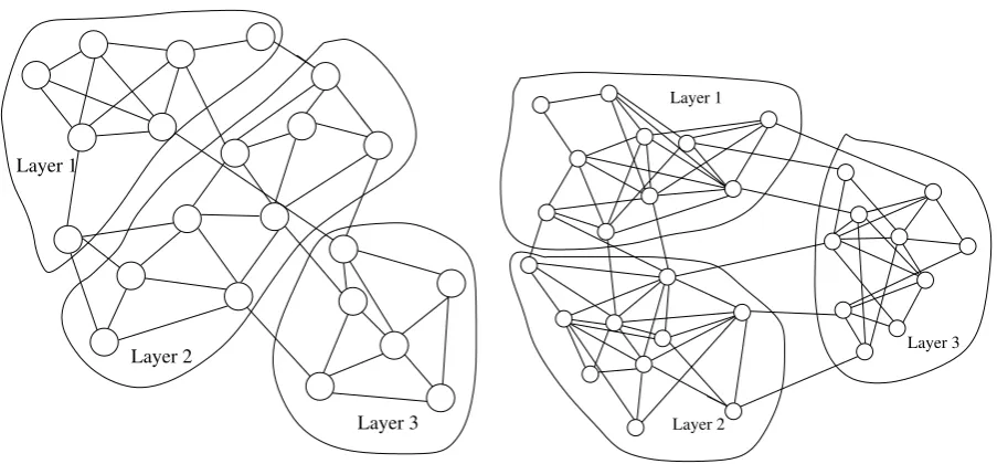
Network topologies. As network topologies, we
L.Maglaras and D.Katsaros
common in the literature [3, 5] and it comprises a very “comfortable” case forSP−BPsince there are more than one shortest path between each pair of nodes. Also, the other two topologies (those in Figure 4) are borrowed from [9] with 22 and 30 nodes, respectively. For the algorithms that use clusters, the clustering is depicted in the figure; the clusters of the grid net are comprised by the four quadrants. In summary, we double the size of the network (from 16 to 30 nodes) and also variate the type of connectivity among clusters, i.e., clusters in a “ring” (16-node net), clusters “almost in a line” (22 -node net), and clusters in a “all-to-all communication”. The performance of the algorithms are similar regardless of the size of the network.
Packet generation. The exogenous arrival processes
at each node are independent Bernoulli processes with rate λ. The destination of every generated packet is randomly chosen. Experiments are also conducted where the destination is chosen according to Zipf’s law in order to simulate the situations where there is a “preference” toward some specific destination node. Since in the conducted experiments with Zipfian-selected destinations, the obtained results show no alteration in the relative performance of the algorithms, all the results we present concern the uniformly-at-random-selected destinations. Different values ofλare chosen according to the number of nodes in the network in order to simulate moderate network traffic. This means that the same λ might represent low load for a small network, but high traffic for a much larger network.
Experimental results. The goal of the experimental evaluation is, apart from testing the delay and throughput performance of all the competing algorithms, to validate all the claims reported in subsection1.1about the misbehavior ofCB−BP andSP−BP. First of all, we examine the impact of parameterA on the performance of the proposed algorithms so as to tune them for the rest of the experiments.
Parameter A - Tuning of the proposed
algo-rithms. Both VoBP and LayBP use the parameter A
to forward packets;LayBP uses it to forward packets to the destination cluster according to layers’ IDs, and in VoBP, the parameter A plays the role of discouraging packets to move backwards in the network. The case of A= 1 corresponds to the traditional backpressure algorithm. We evaluate the performance of the algo-rithms for various A and we present in (Figure 5) the ones concerningLayBP(VoBPalgorithm showed similar performance). The obtained results show no significant gains (either in terms of delay reduction or throughput increase) for values other thanA=2; thus, for the rest of the experiments, we useA=2.
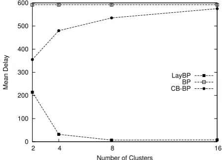
Impact of layer/cluster number. In section 1.1, we
stated that the performance ofCB−BPdeteriorates with the increasing number of clusters; indeed this is the
pattern of its behavior, as shown in Figure6 (tested on a grid topology growing with the number of clusters), where beyond5clusters, the performance of CB−BP is almost 25 times worse than that of LayBP. The same behavior is observed in all the network topologies we simulate. That behavior is predicted by the description in [4]. From this description it is evident that the increased number of clusters implies an increased number of gateways and thus more delays. CB−BP requires a very small constant number of clusters, though most ad hoc clustering algorithms produce a number of clusters which is linear or logarithmic in the number of network nodes. Moreover, the proposed LayBP algorithm performs better as the network is divided in more clusters (see Figure6). This positive characteristic makes the proposed routing algorithm more efficient when combined with most of the automated algorithmic network clustering algorithms.
0 100 200 300 400 500 600
2 4 8 16
Mean Delay
Number of Clusters
LayBP BP CB-BP
Figure 6. Impact of the number of clusters on the grid network topology.
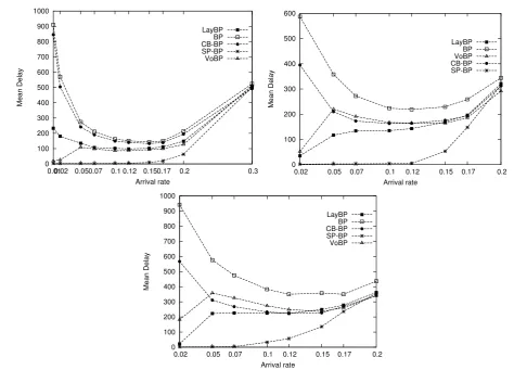
Delay and throughput performance. The plots in
Figure7 depict the delay performance of the competing algorithms. The first generic observation is that the performance of LayBP follows – as a trend – the performance of SP−BP, whereas the performance of CB−BP follows – as a trend – that of the original BP. Additionally, in all cases LayBP is the best policy outperformed only bySP−BP(the theoretically optimal policy).
Layer 3 Layer 1
Layer 2
Layer 1
Layer 2
Layer 3
Figure 4. Network topologies with 22and30nodes.
0 100 200 300 400 500 600 700 800 900 1000
0.01 0.02 0.05 0.07 0.1 0.12 0.15 0.17 0.2 0.3
Mean Delay
Arrival rate A =1 A =2 A =10 A =1.1
0.7 0.75 0.8 0.85 0.9 0.95 1
0.01 0.02 0.05 0.07 0.1 0.12 0.15 0.17 0.2 0.3
Throughput percentage
Arrival rate A =1 A =1.1 A =3 A =5 A =10
Figure 5. Tuning of parameter A - delay prformance of LayBP
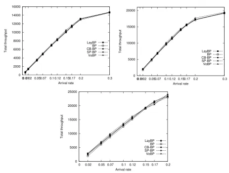
The plots in Figure 8 depict the throughput performance of the competing algorithms. The obvious observation concerns the optimality of all algorithms, including optimality of VoBP and LayBP according to Theorem1.
Maximum end to end delay. The quality of service
(QoS) is defined by the following technical parameters: transmission rate, loss rate,average throughput, maxi-mum end-to-end delay, and maximaxi-mum delay jitter. The maximum end to end delay is an important metric of QoS when critical message transmission is concerned. In Figure9the maximum end to end delay is shown for the 30node topology. We observe that bothBPandCB−BP undergo a high maximum end to end delay for low and moderate traffic. Both proposed algorithms manage to keep the maximum end to end delay low while they even
outperformSP−BPfor moderate network traffic. This is due to the fact that SP−BP guide all packets through short routes leading to congestion over the links that compose these paths and making packets suffer from very long delays.
Impact of topology change (link breakdown). To
validate the claims about the impact of topology on the shortest path backpressure algorithm, we perform an experiment on a small sample network of 10 nodes. The network consists of two clusters; the first includes six nodes and the second cluster includes four nodes. The clusters are connected to each other with only two links. We inactivate one of the two links that connect the two clusters without recalculating the shortest paths among all node pairs. The results presented in Figure10
L.Maglaras and D.Katsaros
0 100 200 300 400 500 600 700 800 900 1000
0.01 0.02 0.05 0.07 0.1 0.12 0.15 0.17 0.2 0.3
Mean Delay
Arrival rate
LayBP BP CB-BP SP-BP VoBP
0 100 200 300 400 500 600
0.02 0.05 0.07 0.1 0.12 0.15 0.17 0.2
Mean Delay
Arrival rate
LayBP BP VoBP CB-BP SP-BP
0 100 200 300 400 500 600 700 800 900 1000
0.02 0.05 0.07 0.1 0.12 0.15 0.17 0.2
Mean Delay
Arrival rate
LayBP BP CB-BP SP-BP VoBP
Figure 7. Delay performance for the three network topologies (16,22and30nodes).
0 500 1000 1500 2000 2500 3000 3500 4000 4500 5000
0.01 0.02 0.05 0.07 0.1 0.12 0.15 0.17
MAX end to end delay
Arrival rate
LayBP SP-BP BP CB-BP VoBP
Figure 9. Maximum end to end delay for the network topology with30nodes
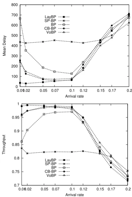
– whereas LayBP maintains its strength. We expected such dramatic changes to have an immediate impact on LayBP also, but LayBP is slighty affected as shown in Figure 10. LayBP is more robust to topology changes
since it does not require exact knowledge of the shortest paths among nodes, but rather shortest paths among clusters.
Since both proposed VoBP and LayBP algorithms favor packets to follow delay efficient paths, but in neither case in a deterministic way, the routing algorithm may get ”stuck” only temporarily due to link breakdown. Both algorithms manage to overcome effectively link breakdown, a common situation in ad hoc networks, for both low and moderate network traffic.
Load Deviation In sensor networks an important
performance metric of a routing algorithm is load devi-ation which is strictly related to energy consumption. Due to the limited energy resources, there is a need for a routing algorithm to balance the load among all nodes while keeping the total load relatively low. In Figure
0 2000 4000 6000 8000 10000 12000 14000 16000
0 0.01 0.02 0.05 0.07 0.1 0.12 0.15 0.17 0.2 0.3
Total throughput
Arrival rate
LayBP BP CB-BP SP-BP VoBP
0 5000 10000 15000 20000
0 0.01 0.02 0.05 0.07 0.1 0.12 0.15 0.17 0.2 0.3
Total throughput
Arrival rate
LayBP BP CB-BP SP-BP VoBP
0 5000 10000 15000 20000 25000
0 0.02 0.05 0.07 0.1 0.12 0.15 0.17 0.2
Total throughput
Arrival rate
LayBP BP CB-BP SP-BP VoBP
Figure 8. Throughput performance for the three network topologies (16,22and30nodes).
consumption. This energy consumption is not calculated in the present simulation and thus the performance of SP−BP is over estimated.
6.2. Dynamic networks
Experimental setting. We evaluate the performance of the cluster-based algorithms in networks with mobile nodes in order to measure the adaptivity of theEL−BP algorithm. It is important here to mention thatEL−BP copes with topology changes in terms of mobility of nodes, which is different than the case evaluated earlier, where a link breakdown was used in order to show the lack of adaptivity of SP−BP algorithm to topology changes. For the evaluations we conduct, we assume that moving nodes update their link information, according to some handshaking mechanism, but are unaware of layer changes.
Network topologies.As network topology, we consider
that illustrated in Figure12. The topology is a network of13nodes where node13moves from layer1(time slot 0) to layer2(time slot1000) and finally to layer3(time slot2000).BP,CB−BP andLayBPare unaware of layer
change while all the active links of the moving node are updated. In EL−BP algorithm, the update procedure runs in every time slot and a moving node joins an appropriate layer according to its neighbor’s information.
Packet generation. In order to have a clear view
of the performance of the cluster-based algorithms we generate in each experiment only one flow from node 1 to the moving node. The exogenous arrival processes are independent Bernoulli processes with rateλ.
Experimental results. Delay and throughput
per-formance.It is clear thatCB−BPbrakes down in
L.Maglaras and D.Katsaros
0 100 200 300 400 500 600 700 800
0.01 0.02 0.05 0.07 0.1 0.12 0.15 0.17 0.2
Mean Delay
Arrival rate LayBP
SP-BP BP CB-BP VoBP
0.7 0.75 0.8 0.85 0.9 0.95 1
0.01 0.02 0.05 0.07 0.1 0.12 0.15 0.17 0.2
Throughput
Arrival rate LayBP
SP-BP BP CB-BP VoBP
Figure 10. Impact of topology changes on the delay and throughput performance ofSP−BP andLayBP.
0 500 1000 1500 2000 2500
0.01 0.02 0.05 0.07 0.1 0.12 0.15 0.17 0.2 0.3
Load deviation
Arrival rate
LayBP BP VoBP CB-BP SP-BP
Figure 11. Load deviation for the grid network topology
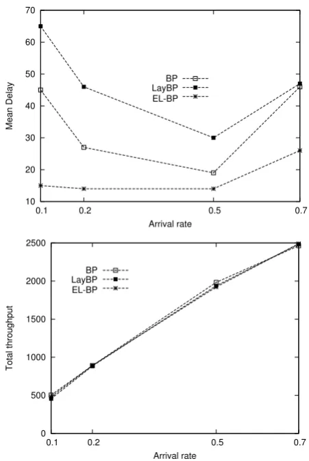
By studying the delay performance of the compared algorithms,we see that LayBP behaves worse than the original BP in cases of moving nodes. The EL−BP algorithm gives the best outcome since a moving node updates the layer information according to its
Figure 12. Dynamic network with3layers.
neighborhood. It is clear that in situations where nodes move along many layers (second dynamic topology) the behavior of LayBP degrades, while EL−BP retains its behavior. All the algorithms give similar outcomes as far as the number of packets successfully delivered per unit time is concerned (Network Throughput).
7. Relevant work
A lot of packet scheduling algorithms have been proposed in the relevant literature. Algorithms for packet scheduling/routing can be classified into data-centric, hierarchical, location-based and those based on network flow or quality of service awareness. The interested reader should refer to [14] for detailed categorization. In data-centric protocols [15], aggregation of data during the relaying of data is utilized. Hierarchical routing algorithms [16] assign different roles to nodes. The nodes are divided into clusters and cluster-heads are assigned with the role of data aggregation and reduction in order to save energy. Location-based [17] protocols on the other hand use the position information of the nodes in order to forward the information to the desired region rather than the whole network. In some approaches, route setup is modeled and solved as a network flow problem [2]. System stability and throughput maximization based on [2] have been exclusively studied [18–21]. Related work on delay-efficient backpressure algorithms is developed in [3, 5,
22–26].
8. Conclusions and future work
10 20 30 40 50 60 70
0.1 0.2 0.5 0.7
Mean Delay
Arrival rate BP LayBP EL-BP
0 500 1000 1500 2000 2500
0.1 0.2 0.5 0.7
Total throughput
Arrival rate BP
LayBP EL-BP
Figure 13. Impact of moving nodes on the delay and on the throughput performance ofBP,LayBP andEL−BP
for the dynamic network with the3 layers.
problems of the backpressure-type algorithms. In this context, the paper describes two algorithms. The first algorithm, namelyVoBP, alleviates the ping-pong effect in packet scheduling. The second algorithm, namely LayBP, investigates the issue of creating layers of nodes and performing backpressure scheduling using the IDs of the layers in order to “push” the packets toward the destination layer.
We conclude that the Voting backpressure performs ideally for low connectivity topologies while the Layered backpressure is a high performance policy compromising a little delay for robustness, low computational complexity and simplicity. Robustness of a routing algorithm in mobility and different connectivity of nodes is a very important aspect of wireless communications and a variation of Layered backpressure algorithm, namely the Enhanced Layered Backpressure, can adapt to moving nodes with exchange of local information between nodes. Our future work involves the combination of voting and layering, i.e., application of
voting inside layers and a more thorough approach on mobile - networks with the use ofEL−BP.
References
[1] Maglaras, L.A. and Katsaros, D. (2011) Layered backpressure scheduling for delay reduction in ad hoc
networks. InWorld of Wireless, Mobile and Multimedia
Networks (WoWMoM), 2011 IEEE International Sym-posium on a (IEEE): 1–9.
[2] Tassiulas, L. and Ephremides, A. (1992) Stability properties of constrained queueing systems and schedul-ing policies for maximum throughput in multihop radio
networks.IEEE TAC 37(12): 1936–1948.
[3] Bui, L., Srikant, R. and Stolyar, A.(2009) Novel architectures and algorithms for delay reduction in
back-pressure scheduling and routing. In INFOCOM 2009,
IEEE (IEEE): 2936–2940.
[4] Ying, L., Srikant, R., Towsley, D. and Liu, S. (2011) Cluster-based back-pressure routing algorithm.
Networking, IEEE/ACM Transactions on 19(6): 1773– 1786.
[5] Ying, L., Shakkottai, S., Reddy, A. and Liu, S. (2011) On combining shortest-path and back-pressure
routing over multihop wireless networks. IEEE/ACM
Transactions on Networking (TON)19(3): 841–854. [6] Huang, L., Moeller, S., Neely, M.J. and
Krish-namachari, B.(2013) Lifo-backpressure achieves
near-optimal utility-delay tradeoff. Networking, IEEE/ACM
Transactions on 21(3): 831–844.
[7] Moeller, S., Sridharan, A., Krishnamachari, B. and Gnawali, O. (2010) Routing without routes:
The backpressure collection protocol. In Proceedings
of the 9th ACM/IEEE International Conference on Information Processing in Sensor Networks (ACM): 279–290.
[8] Athanasopoulou, E.,Bui, L.X.,Ji, T.,Srikant, R. and Stolyar, A. (2013) Back-pressure-based packet-by-packet adaptive routing in communication networks.
Networking, IEEE/ACM Transactions on 21(1): 244– 257.
[9] Amis, A.D.andPrakash, R., Clusterhead selection in wireless ad hoc networks. US Patent 6,829,222 B2, 2004. [10] Basagni, S., Mastrogiovanni, M., Panconesi, A. and Petrioli, C. (2006) Localized protocols for ad hoc clustering and backbone formation: A performance
comparison.IEEE TPDS 17(4): 292–306.
[11] Katsaros, D.,Dimokas, N.andTassiulas, L.(2010) Social network analysis concepts in the design of wireless
ad hoc network protocols. IEEE Network magazine
24(6): 2–9.
[12] Dorigo, M., Maniezzo, V. and Colorni, A. (1996) Ant system: Optimization by a colony of cooperating
agents.IEEE TSMC: Part B 26(1): 29–41.
[13] Neely, M.J., Modiano, E. and Rohrs, C.E.(2005) Dynamic power allocation and routing for time varying
wireless networks.IEEE JSAC 23(1): 89–103.
[14] Akkaya, K.andYounis, M.(2005) A survey on routing
protocols for wireless sensor networks.Ad Hoc Networks
L.Maglaras and D.Katsaros
[15] Intanagonwiwat, C., Govindan, R. and Estrin,
D. (2000) Directed diffusion: a scalable and robust
communication paradigm for sensor networks. In
Proceedings of the 6th annual international conference on Mobile computing and networking (ACM): 56–67. [16] Manjeshwar, A. and Agrawal, D.P. (2001) Teen:
a routing protocol for enhanced efficiency in wireless
sensor networks. InParallel and Distributed Processing
Symposium, International(IEEE Computer Society), 3: 30189a–30189a.
[17] Xu, Y., Heidemann, J. and Estrin, D. (2001) Geography-informed energy conservation for ad hoc
routing. In Proceedings of the 7th annual international
conference on Mobile computing and networking(ACM): 70–84.
[18] Neely, M.J., Modiano, E. and Li, C.P. (2008) Fairness and optimal stochastic control for
heteroge-neous networks. Networking, IEEE/ACM Transactions
on16(2): 396–409.
[19] Stolyar, A.L. (2005) Maximizing queueing network utility subject to stability: Greedy primal-dual
algo-rithm.Queueing Systems 50(4): 401–457.
[20] Markakis, M.G.,Modiano, E.and Tsitsiklis, J.N. (2014) Max-weight scheduling in queueing networks
with heavy-tailed traffic. IEEE/ACM Transactions on
Networking (TON)22(1): 257–270.
[21] Li, R., Eryilmaz, A. and Li, B. (2013) Throughput-optimal wireless scheduling with regulated inter-service
times. In INFOCOM, 2013 Proceedings IEEE: 2616–
2624. doi:10.1109/INFCOM.2013.6567069.
[22] Gupta, G. and Shroff, N. (2009) Delay analysis for
multi-hop wireless networks. InINFOCOM 2009, IEEE:
2356–2364. doi:10.1109/INFCOM.2009.5062162. [23] Huang, L. and Neely, M.J. (2011) Delay efficient
scheduling via redundant constraints in multihop
networks. Performance Evaluation 68(8): 670 –
689. doi:http://dx.doi.org/10.1016/j.peva.2011.02.001.
Special Issue: Modeling and Optimization in Mobile, Ad hoc, and Wireless Networks: selected papers from WiOpt 2010.
[24] Huang, L.and Neely, M.(2011) Delay reduction via lagrange multipliers in stochastic network optimization.
Automatic Control, IEEE Transactions on 56(4): 842– 857. doi:10.1109/TAC.2010.2067371.
[25] Xue, D. and Ekici, E. (2013) Delay-guaranteed cross-layer scheduling in multihop wireless networks.
IEEE/ACM Transactions on Networking (TON)21(6): 1696–1707.
[26] Jones, N.M., Paschos, G.S., Shrader, B. and Modiano, E. (2014) An overlay architecture for
throughput optimal multipath routing. In Proceedings