Estimating the evidence of selection and the reliability of inference in unigenic evolution

R E S E A R C H

Open Access

Estimating the evidence of selection and the

reliability of inference in unigenic evolution

Andrew D Fernandes

, Benjamin P Kleinstiver

, David R Edgell

, Lindi M Wahl

, Gregory B Gloor

Abstract

Background:Unigenic evolution is a large-scale mutagenesis experiment used to identify residues that are potentially important for protein function. Both currently-used methods for the analysis of unigenic evolution data analyze‘windows’of contiguous sites, a strategy that increases statistical power but incorrectly assumes that functionally-critical sites are contiguous. In addition, both methods require the questionable assumption of asymptotically-large sample size due to the presumption of approximate normality.

Results:We develop a novel approach, termed the Evidence of Selection (EoS), removing the assumption that functionally important sites are adjacent in sequence and and explicitly modelling the effects of limited sample-size. Precise statistical derivations show that the EoS score can be easily interpreted as an expected log-odds-ratio between two competing hypotheses, namely, the hypothetical presence or absence of functional selection for a given site. Using the EoS score, we then develop selection criteria by which functionally-important yet non-adjacent sites can be identified. An approximate power analysis is also developed to estimate the reliability of inference given the data. We validate and demonstrate the the practical utility of our method by analysis of the homing endonucleaseI-Bmol, comparing our predictions with the results of existing methods.

Conclusions:Our method is able to assess both the evidence of selection at individual amino acid sites and estimate the reliability of those inferences. Experimental validation withI-Bmol proves its utility to identify functionally-important residues of poorly characterized proteins, demonstrating increased sensitivity over previous methods without loss of specificity. With the ability to guide the selection of precise experimental mutagenesis conditions, our method helps make unigenic analysis a more broadly applicable technique with which to probe protein function.

Availability:Software to compute, plot, and summarize EoS data is available as an open-source package called

‘unigenic’for the‘R’ programming language at http://www.fernandes.org/txp/article/13/an-analytical-framework-for-unigenic-evolution.

Background

One of the principal reasons for studying molecular evo-lution is that the function of a novel protein can be deduced, in part, by comparing it with a similar pre-viously-characterized protein. But what recourse do we have if the novel protein does not exhibit significant sequence similarity to other proteins? More problemati-cally, what if it is similar only to proteins of unknown function? In practice, even when the novel protein shares regions of extensive similarity to proteins of

known function, it may be difficult to elucidate the importance of individual sites in the novel protein.

Unigenic Evolution

One innovative experimental approach that can help identify specific domains or residues required for func-tion is unigenic evolution, first described and developed by Deminoff et al. [1]. Unigenic evolution can be applied to any protein where the loss of function can be used as a selectable phenotype [1-5].

The procedure consists of random mutagenesis and amplification of a single wild-type sequence via muta-genic polymerase chain reaction (PCR) with subsequent cloning and functional selection [6]. Functional clones

* Correspondence: [email protected]

1

Department of Biochemistry, The University of Western Ontario, N6A 5C1 Canada

Full list of author information is available at the end of the article

are isolated and characterized by DNA sequencing. In contrast to traditional structure-based mutagenesis screening, unigenic evolution experiments produce an

unbiased estimate of functionally-important residues regardless of putative structural role or conservation.

Deminoff’s Analysis

The selection process ensures that, in functional clones, amino acids essential for function will be conserved rela-tive to non-essential sites. However, differential mutation sensitivity can be caused by more than structural or func-tional constraints. Mutation rates of residues may differ due to differential transition/transversion rates, codon usage, and genetic code degeneracy. To correct for these confounding factors, Deminoffet al. developed a statisti-cal analysis that compared the expected versus the observed mutation frequency for each codon, where the expected frequencies were derived from a population of clones that had not been subject to selection.

Deminoffet al. clearly demonstrated the importance of accounting for non-uniform transition versus transver-sion probabilities when computing expected mutational frequencies. To increase the inferential power of their analyses, they also developed a‘sliding-window’c2 -analy-sis, binning together a‘window’of adjacent codons, assuming that residues critical for protein function would be nearby in primary structure. By comparing the prob-abilities ofsilentversusmissensemutation in these win-dows, regions of either restrained or excessive mutability were identified as hypo- or hyper-mutable, respectively.

Behrsin’s Analysis

The subsequent analysis of Behrsin et al. [7] advanced the statistical framework of Deminoff et al. by improv-ing three key features. These features were (a) the fixed window size of thec2-analysis, and (b) the effect of sam-ple-size on the codon mutation probability, and (c) accounting for multiple nucleotide mutations per codon. First, window size for thec2-analysis was addressed by using windows of different sizes and comparing esti-mated false-discovery rates. The ‘best’ window was selected via tradeoff between the estimated sensitivity and specificity for classifying hypo- or hyper-mutable residues. Second, nucleotide substitution frequencies were computed using the continuity correction of Yates [8] resulting in more consistent codon mutation fre-quencies. Third, codon mutation frequencies were com-puted analytically from nucleotide substitution frequencies without the assumption that only one sub-stitution per codon was likely.

Further Improvements

The statistical framework of Deminoff et al. and the modifications suggested by Behrsinet al. allow for the

reliable identification of hypo-mutable regions via unigenic evolution. Nonetheless, these state-of-the-art analyses suffer from some deficiencies, from a statistical perspective, that could result in either erroneous or mis-leading conclusions. The goal of this work is to develop a statistically rigorous method for the analysis of uni-genic evolution data, improving upon existing techni-ques by

1. relaxing the assumption that sample sizes are large enough such that asymptotic normality neces-sarily applies,

2. relaxing the assumption that selection-sensitive regions of a protein are contiguous,

3. clarifying the relationship between Fisher-stylep -values and Neyman-Pearson Type-I and Type-II error probabilities with regard to testing hypotheses of functional selection,

4. relaxing the the assumption that the PCR amplifi-cation protocol does not meaningfully affect muta-tion probabilities, and

5. addressing the ability to of unigenic evolution to detect hyper-mutability.

We expand upon each of these points, in turn, below. First, both Deminoff et al. and Behrsin et al. equate observed eventrelative counts with the respective event

probabilities. This equivalence is effectively true when either sample sizes are asymptotically large or probabil-ities are non-extreme (not too close to either zero or one). However, experimentally-feasible sample sizes are typically limited to the order of 50-100 replicates (clones) and even the most mutagenic of PCR condi-tions result in low probabilities (≈ 0.001 to 0.01) of point mutation. Therefore it is unlikely that observed counts have a simple relationship with the event fre-quency, even accounting for the continuity correction of Yates [8]. The difficulty of estimating probability para-meters from event-counts when the likelihood of the event is very small is a well-known problem from the inference of binomial and multinomial frequency para-meters [9]. The most obvious consequence of assuming

“counts≈ probabilities” under these constraints is that the normal approximation, on which the c2 statistic is critically dependent, may be invalid enough to yield mis-leading results. At the very least, the sampling variance of the c2 statistic itself is necessarily quite large. The anticipated parameter ranges above, for example, yield a coefficient of variation forc2 to be on the order of 100-300%. An additional problem with equating counts and probabilities is that, in doing so, the analysis of Behrsin

implying that the variance of the mutation count will be on the order of the expected count itself, further degrading the validity (or at least power) of thec2 statis-tic to correctly determine the effect of selection.

Second, the assumption that selection-sensitive regions of a protein are contiguous is incorrect because proteins are three-dimensional amino acid chains where second-ary, tertisecond-ary, and quaternary folds bring distant-in-sequence residues to three-dimensional proximity. Perhaps the most widely known example of function-ally-important yet non-contiguous sites is the catalytic triad of residues in serine proteases such as trypsin [10,11]. Trypsin proteins have three absolutely required residues that form a charge-relay system needed for activity; with respect to the human sequence these are H57, D102, and S195. These three residues are widely separated in sequence, but are adjacent in the 3 D fold of the protein. Furthermore, S195 is surrounded by a conserved set of residues, but H57 and D102 are not. The residues surrounding the H58 and D102 equivalents in other organisms are very different and are drawn from all classes of amino acids. Thus using a‘ window-ing’procedure to identify hypo-mutable regions would fail in the H57 and D102 instances since many different amino acids are tolerated adjacent to an absolutely con-served position in a protein family. If selection-sensitive residues cannotbe presumed contiguous, it is unclear how sites can be partitioned into ‘selected’ and ‘ non-selected’groups while correcting for implicit and combi-natorially-increasing number of multiple comparisons.

Third, the use of a Fisher-style hypothesis test to com-pute ap-value directly is not equivalent to the estima-tion of the Neyman-Pearson Type-I and Type-II error probabilities aand b, respectively [12]. Although often confused in the literature,panda are not interchange-able. Specifically, Fisher’sp-value expresses the probabil-ity of the observed and more extreme data given the null hypothesis, and can be considered a random vari-able whose distribution is uniform on (0, 1) under that null. In contrast, the Neyman-Pearson aand b values directly compare the probability of the observed data given either the null or alternate hypotheses as correct. The value ofamust be fixedbeforethe observations are made and is subject to the minimization ofb. Confusion betweena andpresults in the systematicexaggeration

of evidence against the null hypothesis [13-17].

Fourth, current unigenic evolution analyses treat the mutagenic PCR protocol as a ‘black box’ process that takes a wild-type sequence as input and produces a pool of mutagenized clones as output. However, the physical process of mutagenic PCR via non-proofreading Taq

polymerase imposes significant constraints on the ampli-fication process in turn constrains properties of the final clone population. We show herein that the ultimate

probabilities of the different classes of codon mutation are complicated, nonlinear functions of the Taq misin-corporation probabilities. Given the complicated rela-tionship betweenTaqmisincorporation frequencies and codon mutation frequencies, it is important to deter-mine if the PCR protocol meaningfully constrains observed codon mutation frequencies.

Last, the claim that unigenic evolution can detect hyper-mutability follows the fact that critical values of the c2statistic can be observed due to either too fewor too many observed mutation events. However, muta-genic PCR of a nucleotide sequence is an anisotropic

‘random drift’ through sequence-space. Selection can

only act on the drifting sequence by ‘slowing’ its pro-gression along trajectories that realize less-functional mutants, since these less-functional sequences are pre-ferentially discarded. Neither mutagenic PCR nor func-tional selection are capable of ‘accelerating’ the sequence drift, thus implying that a‘large’ number of observed mutations at a given site, while improbable, are not unexpected. We therefore claim that unigenic evolution is fundamentally incapable of detecting hyper-mutability, positing that unexpectedly-large site-muta-tion counts stem from either ordinary sampling var-iance, or non-modelled systematic, procedural, or other experimental errors.

The statistical framework described herein provides estimates of both the evidence of selection, and the sta-tistical power available to detect that selection, indepen-dently for each codon site. It provides explicit comparisons with internal positive and negative con-trols, thus reducing the impact of systematic or experi-mental errors. It identifiesindividual sites rather than

broad regionsfor follow-up analysis, and can guide wild-type sequence optimization with regard to unigenic mutability. With its emphasis on analytical rigour and its availability as an easy-to-use software add-in package, this work helps to make the analysis of saturating-muta-genesis experiments both statistically sound and broadly accessible.

Results

visualization and summarization, was implemented as a package called unigenic as part of the R statistical soft-ware system [18] and is available under an open-source license.

Overall Procedure

Like previous methods, our procedure begins by esti-mating the ‘background’ nucleotide mutation frequen-cies given by the mutagenic PCR on a control population of clones that arenot subject to functional selection. This population, termed the‘unselected’ popu-lation, serves as a control group that describes expected mutation frequencies under the null hypotheses of ‘no functional selection’. The nucleotidemutation frequen-cies of the unselected clones are used to compute synonymous and nonsynonymous mutation probabilities for the codonsof the wild-type sequence under the null hypothesis. Finally, the observed number of synonymous and nonsynonymous mutations occurring at each codon of the functionally-selected clones are tested to see whether they are more concordant with the null hypoth-esis or a generalized alternative.

The overall procedure of using nucleotide mutation frequencies to estimate codon mutation frequencies was first suggested by Deminoffet al. who argued that ade-quate statistical power could not be realized if only codon-triplet mutations were analyzed. During the development of our method, we tested the hypothesis that synonymous and nonsynonymous mutation counts alone have sufficient power to resolve functional versus nonfunctional proteins. Our test used a site-by-site test of multinomial homogeneity as described by Wolpert [19]. A test of multinomial homogeneity in our context is a test that, given the count of synonymous and nonsy-nonymous mutations at a particular site in both the selected and unselected populations, asks if the the counts are compatible with the hypothesis that the mutation frequencies are equal. This test is unique in that it does not require inferring or comparing frequen-cies directly. Instead,all possible frequencies that are compatible with the data are considered simultaneously. We found, for the experimental system described below, that codon mutation frequencies alone areinsufficientto discriminate between populations. Results of the homo-geneity tests are shown in Additional File 1. This lack of ability to discriminate populations underlies the neces-sity of formulating a null hypothesis via nucleotide mutation frequencies, and confirms the supposition of Deminoffet al..

Experimental System

Complete details of the experimental system and data analyzed in conjunction with the development of our method are presented in Kleinstiver et al. [20]. Briey, our experimental system analyzed the 266 amino acid

GIY-YIG homing endonucleaseI-Bmol[21-23], a site-specific DNA endonuclease consisting of an N-terminal catalytic domain connected by a linker region to a C-terminal DNA-binding domain. The N-C-terminal domain of ≈ 90 amino acids contains the class-defining GIY-YIG motif that is highly conserved in almost all the members of this endonuclease family.I-Bmolbinds to a≈ 38 bp recognition sequence (the homing site) and introduces a double-stranded DNA break leaving a sin-gle-stranded 2-nucleotide 3’-overhang. We took advan-tage of the site-specific endonuclease activity ofI-Bmol in the genetic selection to isolate functional variants after 30 cycles of mutagenic PCR. The genetic selection utilizes a chloramphenicol resistance plasmid (pExp) to express wild-type I-Bmolor mutant variants, and a second ampicillin resistant compatible plasmid (pTox) that contains the I-Bmol homing site. pTox also encodes a DNA gyrase toxin under the control of an inducible arabinose promoter. Cells that contain both plasmids only survive plating under selective conditions if I-Bmolis functional and can cleavepTox. Cleavage of pToxby I-Bmolgenerates a linear plasmid that is rapidly degraded, thus removing the gyrase toxin and promoting cell survival. If I-Bmolis non-functional andpToxis not linearized, cells will not survive due to the activity of the gyrase toxin. Under non-selective con-ditions, all cells will survive regardless of whether I-Bmolis functional because there is no requirement to cleave the toxic plasmid. Using this genetic selection, we introduced random point-mutations in the I-Bmol coding region by mutagenic PCR, and isolated and sequenced 87 functional ‘selected’clones after plating on selective media. We also isolated and sequenced 87 clones isolated on non-selective media resulting in a pool of‘unselected’clones in order to establish base-line mutagenesis frequencies.

PCR Misincorporation Frequencies

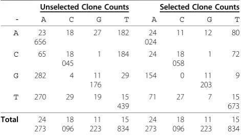
The first step in estimating the nucleotide misincorpora-tion frequencies requires tabulamisincorpora-tion of observed nucleo-tide mutations in the unselected population into the 4 × 4 matrix C, wherecijrepresents the number of observed

product (Σkckj)pijis sufficiently large for alliandj, due

to the same reasoning which underlies the approxima-tion of the binomial with a normal distribuapproxima-tion [24]. Second, this normalization results in only a point-esti-mate ofPand provides no information about the accu-racy of the estimate. Given the low frequency of many mutation events, such as the single observed{C¬ G} event per 11 223 total {any¬ G}events as shown in Table 1, it is doubtful that the condition of‘sufficiently large’holds.

To remedy these difficulties, the columns of P were presumed to be multinomial probabilities of a ‘ black-box’ mutagenic process. Given an ‘input’ wild-type nucleotidej, column jofP gives the multinomial prob-abilities of the resultant ‘output’ clonal nucleotide. Under the hypothesis that the output nucleotide dependsonly on the input nucleotide, each of the four columns of P describe four, independent multinomial distributions.

Estimating multinomial parameters from observed event counts is a well-studied subject. When any (Σkckj) pijis small, as is typical in unigenic evolution data,

tech-niques for multinomial estimation have been thoroughly investigated under various Bayesian frameworks. Follow-ing numerous recommendations in the literature [25], each column ofPis assumed to be Dirichlet-distributed such that our null hypothesis asserts that

H0:P∗j~Dirichlet(C∗j+)for each given wild-type nucleotideej, (1)

where a is a vector of hyperparameters with each component set to 1/2. The justification and derivation of (1) are detailed under the‘Methods’subsection‘ Mul-tinomial Estimation’. Equation (1) defines P as a stan-dard linear Markov operator. Let the four-dimensional

vectorxjdenote the frequencies of the wild-type

nucleo-tidesA, C, G, or T at sitej. In general the wild-type sequence will not display polymorphism, implying that

xj is equal to one of [1, 0, 0, 0], [0, 1, 0, 0], [0, 0, 1, 0],

or [0, 0, 0, 1]. The action ofPonxj, given by standard

matrix-vector multiplication, results in yj =Pxj

repre-senting the frequency of nucleotides expected in site j

within the unselected-clone population.

Modelling the Polymerase

The main difficulty with accepting the hypothesis that the columns ofPdescribeindependentmultinomial pro-cesses is that this hypothesis is not concordant with inspection of observed data. Deminoffet al. specifically noted correlated differences in mutation events that were attributed to differences between transition and transversion processes. Behrsinet al. observed ostensibly the same phenomenon, noting that complementary mis-incorporation events, such as {C¬A} and{G¬ T}, always had similar counts [[7], Table 1]. Again, this similarity was attributed to differences between the mutagenic mechanisms leading to transition and transversion.

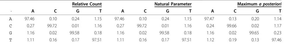
Our observed counts, shown in Table 1, showed a similar pattern. However the reduction to frequencies, as shown in Table 2, suggested the hypothesis that

p_ij p_ij, where _i and j denote the complements of nucleotidesiandj, respectively. Of the sixteen misincor-porations described by P, twelve describe mutations. Differential mutation between transition and transver-sion can only explain differences between the four types of transition-mutations and the eight types of transver-sion-mutation. By itself, such a mechanism is incapable of explaining similarities between complementary-base mutationswithin each of these two classes. Preliminary computational modelling suggested that the similarities betweenpijand pij could be explained by modelling the

overall mutagenic PCR process as the culmination of multiple cycles of error-prone DNA synthesis. Errors in synthesis are presumed to occur via nucleotide misin-corporation byTaq polymerase under conditions opti-mized for mutation [6].

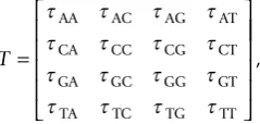
Error-prone nucleotide incorporation byTaq polymer-ase can be modelled if we letτijdenote the relative

fre-quency that the polymerase incorporates nucleotide i

against template-nucleotide j. Collecting these misincor-poration frequencies into matrix T, we compute the PCR mutation frequencies Pas a function of the poly-merase misincorporation frequenciesT resulting in the secondary null hypothesis

′ =

H₀:P P T( ) (2)

Table 1 Sample Misincorporation Counts UnderH0 Unselected Clone Counts Selected Clone Counts

- A C G T A C G T

A 23

656

18 27 182 24 024

11 12 80

C 65 18

045

1 184 24 18 058

1 72

G 282 4 11

176

29 154 0 11 203

9

T 270 29 19 15

439

71 27 7 15 673

Total 24

273 18 096

11 223

15 834

24 273

18 096

11 223

15 834

We denote (2) as a ‘secondary’null hypothesis since T

is estimated using only the unselected clone counts C, thereby still representing the hypothesis of ‘no func-tional selection’. A detailed description of the model underlying H′₀ and the computational challenges asso-ciated with computing the posterior distribution ofPas a function ofT are discussed under the‘Methods’ sub-section‘Modelling PCR via Polymerase’. Again,P under

′

H₀ is defined such that it too is a linear Markov opera-tor. Frequencies Pinferred under H′0 are subtly

differ-ent than those derived under H0 or via relative counts

and are shown in Table 2. Although appearing small, the significance of these differences is difficult to discern by inspection for two reasons. First, codon mutation fre-quencies under the null hypothesis are computed as the product of three nucleotide mutation frequencies. The effect of small differences among the pij parameters is

therefore geometrically amplified with respect to codons. Second, the PCR process is a nonlinear, exponential amplification of misincorporation rates T, implying that small changes in T can result in large changes in both nucleotide and codon mutation frequencies.

Codon Mutation Frequencies

Unigenic evolution presumes that selection operates on protein function and not during transcription or trans-lation. Differences in protein function are caused by nonsynonymous amino acid substitution. Therefore the frequencies of nonsynonymous mutation need to be computed from the given frequencies of independent nucleotide mutation. Although Behrsin et al. provide a number of different sample formulas for deriving codon mutation frequencies given nucleotide frequen-cies, we describe a generalized method of deriving these frequencies for two reasons. First, our framework immediately accommodates different genetic codes, such as mitochondrial or chloroplast. Second, we require ready generalization, beyond the two classes of synonymous or nonsynonymous mutation currently used, for future work.

A codon comprises three contiguous nucleotides within a given reading frame. SinceP is assumed to act

independentlyon nucleotides, the mutagenic PCR pro-cess for codons is concisely represented by

M= ⊗ ⊗P P P, (3)

where M is a 64 × 64 linear Markov operator that operates on the space of codon frequencies and ‘⊗’ denotes the standard Kronecker matrix-product. An explicit depiction of the Kronecker product and how it relates nucleotide mutation to amino acid mutation is shown in Additional File 2. As with nucleotides, given wild-type codon frequencies wj at codon-site j, the

quantity zj = Mwj represents the frequency of site-j

clone codons after mutagenic PCR under the null hypothesis.

The columns of M describe the probabilities that a codon subject to mutagenic PCR will remain identical, mutate synonymously, or mutate nonsynonymously. For example, consider column AGA of M. The standard genetic code translatesAGA to arginine, as do the five additional codons CGT, AGG, CGA, CGG, and CGC. Therefore, given AGA as the wild-type codon, M

describes the probability of either no mutation (identity) or synonymous mutation as

p M i

i i

sn

for CGT AGG CGA CGG CGC

=

∈

∑

{ , , , , , },

AGA

AGA

(4)

and the probability of nonsynonymous mutation aspns

= 1 -psn. Such matrix partitioning is simple to code in

languages supporting named-index array-slicing, such as R [18]. It is also simple to adapt the required bookkeep-ing to any desired genetic code. For computational effi-ciency and ease of notation, we denote psn,jandpns,jto

be the probabilities of synonymous and nonsynonymous mutation at codonj, using the subscripts to clearly dif-ferentiate them from the entries of nucleotide mutation matrixP, above.

Table 2 Estimates for the Expected Nucleotide Mutation Frequency

Relative Count Natural Parameter Maximuma posteriori

- A C G T A C G T A C G T

A 97.46 0.10 0.24 1.15 97.46 0.10 0.24 1.15 97.47 0.13 0.20 1.14

C 0.27 99.72 0.01 1.16 0.27 99.72 0.01 1.16 0.24 99.66 0.02 1.17

G 1.16 0.02 99.58 0.18 1.16 0.02 99.58 0.18 1.16 0.02 99.65 0.23

T 1.11 0.16 0.17 97.51 1.11 0.16 0.17 97.51 1.12 0.19 0.13 97.46

Unit of Analysis

Rather than using only the two classes of synonymous and nonsynonymous mutation, it istheoreticallypossible to compare the observed counts for all 20 amino acids at each codon site. Such a comparison reducesM to a 20 × 64 matrix mapping codons to amino acids. Preli-minary analyses of the≈ 100 clones sequenced in each of our selected and unselected populations, however, showed insufficient power to make meaningful infer-ences at the amino acid level.

Amino acids or synonymous/nonsynonymous muta-tion are not the only possible units of analysis, however. For example, the assumption that selection operates at the protein level implies that the functional assay is independent of transcription or translation efficiency. Future work could easily test this hypothesis by redu-cing M to the three classes of ‘identical’, ‘synonymous but not identical’, and ‘nonsynonymous’. Possibly, even different classes of codons could be defined. The main tradeoff with using more classes for analysis is the requirement for larger sample sizes. However, the basic hypothesis-testing framework described below could be used with only trivial modification.

Alternate Hypothesis

The analysis of a unigenic evolution experiment com-pares observed site-specific mutation counts between two populations. The first population, the control group, is not subject to selection; these are the ‘unselected’ clones and they provide the values of psn,j and pns,j

under the null hypothesis.

The second populationissubject to functional selec-tion and results in a set of ‘selected’clones. The fre-quency of mutation at each codon of the selected population provides an alternate hypothesis that can be compared with expectations under the null.

For codon-sitejwe denote n_snus_,j and n_nsus_,j to be the respective number of observed synonymous and nonsy-nonymous mutations in the unselected population, and

n_snmx_,j and n_nsmx_,j to be the respective number of observed synonymous and nonsynonymous mutations in the selected population. The total number of clones

sequenced from each pool is therefore

nus =n_snus_,j+n_nsus_,j and nmx =nmx_sn,j+nmx_ns,j, both of which are constant for allj.

Likelihood Model

A standard multinomial likelihood model is used to describe the probability of mutation given the total number of clones sequenced and the presumed fre-quency of mutation. For each codon-sitej, this gives

Pr , | ,

!

! !

, ,

, , ,

n n n H

n n n p

j j

j j

snus nsus us

us snus nsus

sn

(

)

( ) ( )

Pr , | ,

!

! !

, ,

, , ,

n n n H

n n n p

j j

j j

snmx nsmx mx

mx sn mx ns mx sn

(

)

( ) ( )

with codon mutations presumed to be mutually inde-pendent. The conditional hypothesis Hdictates the ori-gin of the probability parameters p_snus_,j, p_nsus_,j, p_snmx_,j, and

p_nsmx_,j. Under the nullH=H0 these parameters are

com-puted via nucleotide countsCusing (1). Under the sec-ondary null H= ′H0 they are computed via polymerase

misincorporation frequencies T using (2). Under the alternate hypothesis H =HA, they are inferred using

only the site-specific counts n_snus_,j, nus_ns,j, n_snmx_,j and

n_nsmx_,j, respectively, theoretically accommodatingany

type of selection mechanism.

Therefore under HA the distribution of parameter-pair

p_snk_,j,pk_ns,j

⎡

⎣ ⎤⎦, forkÎ {us, mx}, is

p_snk_,j,p_nsk_,j Dirichlet n_snk_,j,n_nsk_,j ,

⎡

⎣ ⎤⎦

(

)

as discussed previously. Again,a is a vector of hyper-parameters with each component set to 1/2 and the jus-tification and derivation of (7) are detailed under the

‘Methods’subsection‘Multinomial Estimation’.

Note that since parameters inferred underHA

encom-pass arbitrary types of selection, they necessarily overlap with parameters under the null. However, under HA

parameters p_sn,k _j and pk_ns,j are relatively diffuse since they are estimated from≈100 sequenced clones. Under

H0 or H′0 these same parameters are estimated by≈20

000 nucleotide misincorporations and are thus more precisely determined.

Lastly, we test both selected and unselected popula-tions for consistency between hypotheses since doing so treats the unselected population as a negative control. This helps identify possible systematic or experimental errors during cloning or sequencing, thereby reducing false signals of selection.

Evidence of Selection

Given prior probabilities Pr(HA) and Pr(H0) that either

conjunction with standard likelihood ratios can be used to compute

Pr , , Pr

Pr

, | ,

,

, , , ,

, ,

n n p p n n

n H H

j k j k j k j k j k j k k A A

sn ns sn ns

sn ns

( ) ( )

|| ,

| , |

, , Pr

Pr ,

, ,

, ,

n H H

H n

p p

n n p

k A k j k j k j k j k sn ns

sn ns sn

0 0

( ) ( )

= ,, ,

, , , ,

,

Pr | , | , , ,

j k j k j k j k j k j k k p

n n p p

H n

ns

sn ns sn ns

( )

( 0 )

(8)

the relative probabilities of the hypotheses at codon j, given the dataandparameter values. UsuallyPr(HA) and

Pr(H0) are set equal to each other in the absence of

other information. However, parameter values are not known precisely but have posterior distributions. Taking logarithms of (8) and integrating over these posteriors results in

Rkj =

∫∫

( )

[

]

[

]



sn ns sn ns 0

where



R n n n p p H H

n n j k j k j k j k A A j k k

= Pr

(

)

Pr

, | ,

,

, , , ,

,

sn ns sn ns

sn ns,,j| , ,, , , Pr( )

k j k j k k

n p_sn p_ns H₀ H₀

(

)

giving

R H n n

H n n

j

k A j

k j k j k j k = ⎡ ⎣ ⎢ ⎢ ⎤ ⎦ ⎥ ⎥

(

)

(

)

log | ,

| , , Pr Pr , , , , sn ns sn ns 0 (9)

the expected log-odds-ratio ofHA versusH0 given the

number of observed mutations for codon j in clone-population k. We call Rjk the Evidence of Selection

(EoS) for codonjin clone-population k.

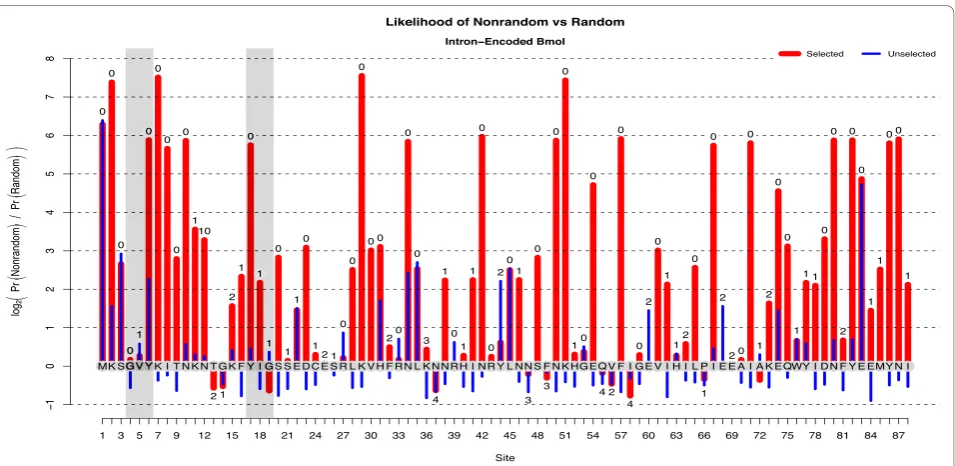
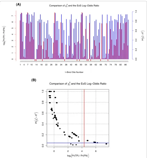
The EoS score is the primary criterion used by Klein-stiveret al. [20] to identify functionally-relevant residues in I-Bmolvia unigenic evolution. The EoS scores for the first 88 sites ofI-Bmolare shown in Figure 1.

Although (9) is derived using similar principles to Kullback’s and Leibler’s information divergence [26], a similarity exploited below, it is not obvious why integrating the logarithm of (8) over the posterior parameter estimates is a statistically valid procedure. Briey, this integration is justified because log-odds-ratios are isomorphic to standard Euclidean vector spaces [27-29] and can be‘added’ together in a mean-ingful manner that is consistent with the fundamental laws of probability. For example, consider two

differ-ent point-values for pk _j pk _j

HA

sn,, ns,

⎡

⎣ ⎤⎦ and

pk _j pk _j

H

sn,, ns,

⎡

⎣ ⎤⎦ 0

for the integrand of (9). The first point-value yields an odds-ratio of 10:1, indicating a preference for HA, while the second point-value yields

1:10, indicating a preference for H0. Intuitively, if

these two point-estimates were the only parameter values available, we expect the ‘total’odds-ratio to be 1:1. In other words, the data supports both hypoth-eses equally. This ‘total’ is represented exactly by summing the log-odds-ratios, where

log ( )101 +log (1010) : log ( )11 log (1010) 1 1: ,

(

)

(

)

as expected. Such ‘addition’ holds over very general conditions, and underlies not only the validity of (9) for computing Rk_j, but the foundations of information the-ory and the Kullback-Leibler divergence [30].

The interpretation of log-odds-ratios in the literature is traditionally taken as the‘strength of evidence’ favor-ing one hypothesis over another [31,32]. However, since

HAdescribes a general case that embeds H0 as an

alter-native, this traditional interpretation is inappropriate for

Rk_j. Instead, Rk_j is interpreted in the Neyman-Pearson sense, where it describes the relative probability of cor-rectly classifying a specific observation to be due to eitherHAor H0. Interpretation of Rj

k

requires consider-ing three cases:

• Rjk>0: HA is more probable than H0, with Rkj

being the expected logarithm of the true-positive to false-negative ratio for determining whether or not selection operated on the site.

• R_jk0: BothHAandH0 are supported equally by

the data, implying that the data are unable to differ-entiate between whether or not functional selection has occurred.

• Rkj <0: Although technically implying that H0 is

more probable thanHA, the embedding ofH0within

HA implies that negative values of Rjk will likely

have small magnitudes and can be interpreted as if they are zero.

The interpretation of Rk_j <0 follows from Gibbs’ inequality which guarantees the probability-weighted average of R_jk

(

)

and the data of Kleinstiver et al. [20], large negative values for R_jk have not been observed.

A concrete example of interpreting Rk_j is given by examining theGIY-YIGmotif ofI-Bmol, shown grey-highlighted in Figure 1. Precise values of R_jk along with the expected and observed number of nonsynonymous mutations are given in Additional File 3. Although all six motif-residues are well conserved within this homing endonuclease family, Figure 1 shows that unigenic selec-tion is only detectable for the tyrosine residues which show posterior odds-ratios of 25.8 ≈ 59.7-to-one in favour of selection. The four-to-one odds ratio or less shown by the other residues is by general convention considered to be negligible.

This example highlights how the lack of evidence of selection does not imply a lack of functional importance. Lack of evidence is precisely that: there is not enough data to classify a given site as either‘ impor-tant’or ‘unimportant’. Often, as can be seen with the GIY-YIGmotif, many codons are intrinsically resistant to nonsynonymous changes under mutagenic PCR. The glycine residues, for example, can be seen to have had five mutations at site 4 in the selected population but less than one of them is expected to be nonsynonymous.

Much of the reason that selection is detectable at the tyrosine residues is the large number of expected nonsy-nonymous mutations, a number principally dependent on the tyrosine codon’s nucleotide composition. The number of nonsynonymous mutations expected for dif-ferent clone population sizes is shown in Additional File 4 and is described more fully later.

We note an advantage of our method over previous work is shown by examining R_jk values for the unse-lectedpopulation. There, the negligible values of Rkj act

as a negative control indicating‘no evidence of selection’ when no selection is actually present. Large values of

Rk_j in the unselected clone population would indicate the presence of systematic bias or experimental errors.

Power and Reliability

The similarity of (9) to a Kullback-Leibler divergence can be exploited to estimate the statistical power for inferring selection at a given site. The integrand of (9), for given parameter values and where Pr(HA) = Pr(H0),

is the log-ratio of multinomial likelihoods. Taking the expectation of this log-ratio over the space of all possi-ble data given HA yields a point-estimate of the

Kull-back-Leibler divergence

Figure 1The Evidence of Selection for I-Bmol. Posterior log2-odds-ratio EoS score Rmx_j for the first 88 amino acid sites ofI-Bmolfor both

Rmxj

where



L n

n

n n p p H

n n

j k

j k

j k

j k

A j

k j k

k k

= Pr

(

)

Pr

, | ,

, |

, , , ,

, ,

sn ns sn ns

sn ns ,, ,

, ,

, ,

pk_snj p_nsk _j H₀

(

)

⎡

⎣ ⎢ ⎢

⎤

⎦ ⎥ ⎥

which can itself be integrated over the multinomial parameter posteriors, as before, to yield the overall expected divergence DHA. As interpreted by Kullback

[26,30], D_H

A measures how distinguishable two

ran-dom variables are in terms of the expected true-positive versus false-negative rate. Conditioning onH0, the

com-plementary D_H

0 provides the expected true-negative versus false-positive rate. Together, D_HA and D_H0 spe-cify the confusion matrix between hypotheses, thus pro-viding a detailed power estimate of hypothesis distinguishability.

Another way of interpreting the per-site values of

D_H

A and DH0 is through the idea of ‘reliability’. If we assume that the mutation frequencies estimated viaHA

andH0are even approximately correct, DHA and DH0 quantify the estimated robustness of Rk_j by averaging it over the range of expected nonsynonymous mutation counts. The estimated reliability of the EoS score for I-Bmolis shown in Figure 2. For the selected population, the true-positive reliability scores are highly correlated with their respective Rk_j values, agreeing with the intui-tive notion that the greater the evidence of selection, the more likely that that evidence is reliable.

Effect of Sample Size

To help elucidate the practicaleffects of sample size on EoS values with respect to both the unselected and selected clone population, subsampled clone populations were analyzed with results displayed in Additional File 5. In brief, even as few as 10 unselected clones (yielding 100-300 nucleotide misincorporation counts) were cap-able of giving reasoncap-able estimates of parameter matrix

T and sensitivity. Reasonable specificity however, as judged by the ability to correctly detect selection of the methionine start signal, was not achieved with fewer than all 87 of the unselected clones. With respect to the misincorporation frequencies estimated from the counts in Table 1, percentiles of the likely number of nonsy-nonymous mutations observed for given clone

population sizes under the null hypothesis of‘no selec-tion’are shown in Additional File 4. This table shows considerable non-normality that is particularly pro-nounced for mutation-resistant codons, highlighting the requirement (and opportunity) to ‘tune’ the effective selection pressure on individual residues by adjusting codon composition. Again, since normality is a require-ment for the validity of c2-based statistics, the non-nor-mality displayed by many residues even under very large sample sizes (> 500 clones) calls the validity of such analyses into question.

Global Insights from Local

The derivation of Rjk (EoS), although a primary result

of this work, is alone insufficient to analyze unigenic evolution data. The following subsections provide addi-tional computaaddi-tional details required for a complete analysis.

Selecting Selected Sites

One of the major shortcomings of previous work was the difficulty of discerning which groups of sites were under functional selection given statistical procedures that were designed under the assumption of site-inde-pendence. Given ncodons with ‘sufficiently-high’ EoS score, there aren! different ways to partition those n

codons into important and functionally-unimportant categories and thereby estimate the false-discovery rate. This huge number of partitions implies that traditional techniques for multiple-comparison cor-rection reduce statistical power to impractically low levels.

The‘windowing’analyses of Deminoffet al. and Behr-sinet al. were used to constrain the number of required multiple-test corrections to a reasonable level.

The principal benefit of using R_jk as the evidence of selection is that the additive nature of log-odds-ratios imply that Rjk values can simply be summed across all

sitesjof interest without unnecessary loss of inferential power. IfJ denotes the set of sites-of-interest, then the combined log-odds-ratio

R_Jk R_jk

j J

=

∈

∑

can be interpreted as the log of relative probability that all sites in J were observed due to the action of selection as hypothesized by HA. Unlike traditional

mul-tiple-test corrections such as Bonferroni’s, RJk

The benefit of using RJk as evidence of selection in

unigenic evolution is clearly demonstrated by Figure eight of Kleinstiver et al. [20] via the functional analysis ofI-Bmol. There, assays of N12 D, S20Q, H31A, I67N, and I71N mutants clearly implicate these residues, as identified by their EoS scores, as functionally important. This importance is seen experimentally as the genera-tion of a phenotype distinct from wild-type for each respective mutant.

Note that RJk systematically underestimates the

pos-terior odds that a set of sites are subject to selection since it predicates on all sites of Jbeing selected. If only one or two of these sites were false-positives, RJk

behaves as if all sites J were false-positives, artificially reducing the actual true-positive rate. It is straightfor-ward, though tedious, to compute precise overall true-positive rate given R_jk for jÎ J. However, in practice

Figure 2The Reliability of Inference for I-BmoI. Estimates of statistical power (reliability of inference) forI-Bmol, for both selected and unselected clone populations.‘Nonrandom’associations are presumed due to the alternate hypothesis while‘random’associations are presumed due to the null. Power is computed as the expected log2-odds-ratio for either true-positive versus false-negative (mauve) or true-negative versus

false-positive (teal).(A)For the selected sequences, the true-positive ratio is strongly correlated with the posterior log2-odds-ratio shown in

the individual values Rkj generally display a sharp

boundary between‘large’and‘small’values, making the choice of putative functional sites straightforward via simple inspection (see Figure 1).

We further note that neither Rk_j or R_Jk are directly comparable to either the H-scores or c2-values of Deminoffet al. or Behrsinet al. since the former tion explicitly on observed data while the latter condi-tion on unobserved hypothetical data. Restated, the former is congruent to a Type-I error probability (a), while the latter is a Fisher-type significance p-value. Although correlated, these two values have no simple relationship.

Protein Mutation Count

For the experimental conditions used herein, nonsynon-ymous mutation probabilities varied between ≈ 0-10%, depending on the given codon. These mutation

probabilities in turn determine , the total number of nonsynonymous mutations expected in the overall pro-tein. The overall mutation count is an important experi-mental diagnostic since too few mutations lead to inefficient mutagenesis and high sequencing costs, while too many mutations result in nearly-certain functional knockout. The simplest method of computing the distri-bution of uses standard Monte Carlo techniques to performin silico mutagenesis of the wild-type sequence given nucleotide mutation parameters underH0.

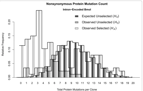
The distributions of total protein mutations per clone, both expected and observed for the unselected clones under H0 and observed for the selected clones under

HA, are shown in Figure 3. UnderH0 > 96.7% of clones

are expected to have between 4-16 nonsynonymous mutations, inclusive, within the 266 amino acid sites of I-Bmol. Expected and observed distributions underH0

were very similar, especially considering the small sam-ple-size of 87 clones that was available to estimate the distribution. The selected population, under HA,

Figure 3The Expected Mutation Count Distribution for I-Bmol. The expected distribution of total nonsynonymous mutations per clone () forI-Bmolunder the null hypothesis of‘no selection’, the observed mutation count frequencies for the unselected clones, and the observed mutation count frequencies for the selected clones under the alternate hypothesis. Over 96.7% of clones are expected to have between 4-16 nonsynonymous mutations, inclusive, within the 266 amino acid sites ofI-Bmol. Expected and observed distributions underH0were very

displayed a marked decrease in the number of muta-tions, with > 95% of clones having seven or fewer mutations.

Note that like previous analyses, both our null and alternate hypotheses assume site-independence among mutations. Second-site suppression or other modes of site-interaction are not taken into account. Under rare conditions for I-Bmol, it is possible that up to 20 mutations could be expected for this 266-site protein, making it likely that interaction effects are non-negligi-ble factors of selection.

Comparison with Previous Work

A comparison of our EoS values with thec2-based sta-tistics of previous work is shown in Figure 4. In a broad sense, non-binned site-specific c2 statistics with one degree of freedom and EoS values appear to be highly predictive of one another. However, their interpretation and use are very different, especially with respect to sen-sitivity-vs.-specificity and multiple-comparison correc-tion. For example, the single degree of freedom used in Figure 4 dictates a wide sampling variance for the ₁2

statistic, translating to a very high predicted false-posi-tive rate. Binning adjacent sites such as done by Behrsin

et al. [7] could reduce the false positive rate but only at the expense of a concomitantly-lower true positive rate

–the classic sensitivity versus specificity tradeoff. Nonetheless we note that even using the highly-sensi-tive ₁2 _{values, only 10 of the 266 sites exceeded the}

critical p-value of p < 0.05, whereas using EoS, 41 of 266 sites exceeded the critical log-odds ratio of 20:1 (see Figure 4). Thus previous methods identify less than 25% of sites identified with EoS. Most importantly, the addi-tional sensitivity of the EoS value appearswithout detri-ment to specificity, as shown by the estimated false-positive to true-negative ratios in Figure 1, ratios that are impractical to estimate via previous methods. Thus our method appears both significantly more sensitive

andselective than previous work for the unigenic analy-sis ofI-Bmol.

Another advantage of EoS values overc2-based statis-tics is illustrated by the nontrivial comparison of thep< 0.05 and 20:1 odds-ratio critical values shown in Figure 4. Although detailed interpretations and the differences thereof have already been discussed, in the particular case of theI-Bmoldata shown in Figure 4 it is impor-tant to realize that Bonferroni correction of the ₁2

values would render none of the sites significant by con-ventional measures. In contrast, the log-odds ratio shows comparatively little power-loss due to multiple-comparison correction.

From a theoretical viewpoint, another advantage of the EoS value is that it deals with a very direct statistical question: how likely are the observed data given the model? Unrealistic EoS values are necessary and suffi-cient to diagnose unrealistic assumptions in the mathe-matical description of unigenic evolution. In contrast, summary statistics such asc2 values similarly condition on model accuracy, but necessarily furthercondition on the statistic being a good indicator of the phenomenon under investigation–in this case, selection. Thus unrea-listic values ofc2can be similarly be attributed to model mis-specification, but could also be due to the inade-quacy of the chosen test statistic.

Additional Results

Although the main result of this work is the EoS score

Rkj and its associated reliability estimate, two additional

results were discovered during the analysis of the I-Bmol system. The first result concerned differences betweenH0 and H′0, the second concerned the

treat-ment of stop codons.

Polymerase Versus PCR Modelling

A surprising result was that Rjk and power estimates

computed under H0, modelling only the overall PCR

process, and H′0, modelling the misincorporation of

nucleotides by Taqpolymerase, were effectively indistin-guishable. Observed log-odds differences were all on the order of the Monte Carlo sampling-variance cutoff used to estimate each and were therefore effectively zero. The inability of the data to discriminate betweenH0 and H′0

implies that there is no effective difference between these models. In effect, there is no meaningful difference in the Rkj scores computed by either (a) treating

muta-genic PCR as a ‘black-box’ process or (b) modelling mutagenic PCR to be be consistent with the action of error-prone polymerase.

This finding is surprising because modelling the effect of the polymerase over multiple PCR cycles appears to be required in order to produce mutation frequencies, such as those in Table 2, where complementary-base frequencies are always almost equal. The similarity of respective Rk_j values imply that differences between estimates ofPunder each hypothesis are negligible com-pared to the magnitude of uncertainty inherent in esti-matingPgiven C.

Figure 4A Comparison of EoS values with Prior Work. Comparison of the EoS value with the 

1

2 _{statistics of prior work.(A)A per-site}

comparison of EoS values (left, red) with 

1

2 _{statistics (blue, right). Both values are plotted such that larger values roughly indicate‘greater}

significance_’.(B)EoS and 

1

2 _{values are highly though non-linearly correlated, but arenotcomparable in terms of‘significance’. Specifically,}

while only 10/266 sites exceed the 

1

2 _{critical value ofp< 0.05 as shown by the blue horizontal line, 41/266 sites showed a posterior odds}

ratio of 20:1 or greater as shown by the red vertical line. We emphasize that binning adjacent sites would increase the specificity of thec2

cytosine deamination via thermal decomposition during PCR cycling [33-35] provides a credible, alternative mutation mechanism. In this case the non-proofreading property ofTaqwould be a more important factor than its misincorporation characteristics.

Optimizing the experimental conditions under which mutagenesis occurs can have important consequences in the efficiency and expected outcome of unigenic evolu-tion. For example, note the ≈ 100-fold difference between{C¬ G}and{G¬ A}mutation frequencies shown in Table 2. Small changes in mutation frequen-cies due to different mutagenic protocols could effect large changes in the distribution of mutant codons, sug-gesting that future work should investigate mechanisms to elucidate the factors affecting the precise characteris-tics of mutagenic PCR.

Stop Codon Assumption

One of the more significant assumptions of this work is the presumption that the effect of stop codons can be ignored. Unlike other mutations, the appearance of a premature stop codon affects every subsequent codon, negates our assumption of site-independence, and likely results in a complete loss of function. For the system examined herein and in Kleinstiveret al. [20], we found that the frequency of stop codon production was suffi-ciently small as to not significantly affect results or interpretation. Given this putatively small effect, a more exact treatment of stop codons and their functional effects are left for future work since a correct and rigor-ous treatment would likely add considerable algebraic and computational complexity.

Conclusions

From an experimental point of view, the evidence of selection at a given site represents only part of the required information; in general, the reliability of that evidence must also be assessed. Quantifying reliability is important since small sample sizes, mutation events that are too rare to be reliably estimated, and the effects of multiple comparisons can complicate the interpretation of unigenic evolution experiments. Our method, which computes both evidence and reliability, represents a sig-nificant advance over previous work since it simulta-neously assesses both the evidence of selection and the reliability of inference.

Experimental validation of our methods was provided via analysis of the poorly-characterized homing endonu-clease I-Bmol, where previously-described methods from the literature were unable to elucidate function-ally-critical residues. With the ability to guide the selec-tion of precise experimental mutagenesis condiselec-tions, our method makes unigenic analysis a more broadly applic-able technique with which to probe protein function.

Methods

Herein we provide technical and implementation details for our analytical framework, the most important of which are (a) the estimation of multinomial frequencies from counts, (b) our model of mutagenic PCR via the action of an error-prone polymerase, and (c) selecting the prior and sampling the posterior of the polymerase misincorporation frequencies.

Multinomial Estimation

The estimation of multinomial frequencies from counts is one of the oldest subjects in statistics. When asympto-tically-many observations are available, both Bayesian and frequentist methods infer nearly identical parameter values, where frequencies are simply proportional to counts. However, when observations are rare, prior beliefs will always, necessarily significantly affect inferred results. These effects, thoroughly described by Jaynes [36], can be understood though a simple example. Sup-pose that 10 000 clones were sequenced of which 5000 were found to have nonsynonymous mutations at a given site. Using the normal approximation to the bino-mial distribution both the mean frequency of nonsynon-ymous mutation and its standard error are easily computed with high accuracy. However, if onlyone non-synonymous mutation had been observed, the actual fre-quency of mutation is not clear since mutation frequencies of 0.5, 1, or 2 mutations per 10000 clones, a range of 400%, are all realistic and compatible with the given data. Prior belief that the mutation rate should be

‘somewhat high’will favor the higher rate, surprise at seeinganymutation would imply the lower rate is more believable.

The consensus in the statistical community is now that there is no ‘best’ notion of ‘prior ignorance’ that can be universally considered correct [37,38]. Instead, research has focused on developing methods with pre-cise and well-characterized assumptions in order to minimize, in some sense, the influence of prior tions on the inference. These well-charactered assump-tions are called‘objective’or ‘reference’priors and are the type of prior we choose as a basis for inferring both multinomial nucleotide mutation frequencies and nonsy-nonymous codon mutation frequencies.

Ifprepresents a set of multinomial frequencies andn

a set of observed counts, then Bayes’ Theorem tells us that

Pr

(

)

(

)

( )

[25] found thatp~ Dirichlet(a) with all components of vector aset to 1/2 was a prior that formally minimized the inuence of the prior on the posterior Pr(p|n). This specific prior was found to be invariant to reparameteri-zation and is identical to the one derived by Jeffreys [39].

From an experimental viewpoint, invariance to repara-meterization is an critical requirement for inferring fre-quencies from counts since the property implies that the sameinference would be made if, for example, rela-tive mutationrateshad been estimated rather than fre-quencies. Any other choice of prior would yield different posterior values ofpeven when given identical data.

For the multinomial distribution with the objective reference prior above, the posterior has the simple form

p n| ~ Dirichlet

(

)

Again, onlya = 1/2 formally maximizes the informa-tion ‘extracted’from the counts n. The expected value of these posterior relative frequencies is

⎡⎣log

( )

∑

(

)

(

∑

(

)

)

for each frequency-componenti, whereψ denotes the digamma function. Equation (13) is termed the‘natural’ parameter mean for p, and whenni is sufficiently large

it is approximately equal to ni/Σi ni. This similarity is

evident when comparing the‘Relative Count’and‘ Nat-ural Parameter’estimates for nucleotide mutation fre-quencies in Table 2 where all four multinomial parameter set estimates agree to within 1%. However, for codon mutation counts on the order of 0-2 observa-tions per 100 clones, differences between estimates can be considerable.

Modelling PCR via Polymerase

Modelling the full mutagenic PCR process requires for-mally describing both the process of nucleotide misin-corporation via polymerase and the action of multiple cycles of denaturation, synthesis, and reassociation that are the basis of PCR. Our model uses a Bayesian frame-work that explicitly accounts for the rarity of nonsynon-ymous mutations to infer parameter values of this model.

Polymerase Misincorporation

Mutagenic PCR is composed of of multiple cycles of low-fidelity Taq-based amplification. The model we adopt assumes that under mutagenic conditions [6]Taq

polymerase

•induces errorsonlyby nucleotide misincorporation,

•has negligible slippage, stutter, or other errors due to repeats,

• and has site-independent misincorporation probabilities.

The assumption that slippage and stutter are negligi-ble is substantiated by previous studies of Taq errors [6,34] and visual inspection of our data. The assumption that nucleotide misincorporation events are independent is somewhat stronger since it may be argued that spatial distortions induced by template-adduct mispairing affect subsequent DNA synthesis. However, inspection shows misincorporation events to be sufficiently rare that this effect, if it exists, is of sufficiently small magnitude as to be negligible.

A single nucleotide is represented as the four-dimen-sional probability column-vector pthat comprises the probability of that nucleotide being one of the four nucleotides A, C, G,orT. The action ofTaq polymer-ase on template pis modelled as a linear Markov opera-tor T that pairs adduct q =Tp against the template during synthesis. Polymerase operatorThas the explicit representation

T =

⎡

⎣ ⎢ ⎢ ⎢ ⎢

⎤

⎦

   

   

   

   

AA AC AG AT

CA CC CG CT

GA GC GG GT

TA TC TG TT

⎥⎥ ⎥ ⎥ ⎥

, (14)

whereτijdenotes the probability that

adduct-nucleo-tideiis base-paired to template nucleotidej.

With this notation, the columns of T sum to one. Further, since misincorporation events are rare, the counter-diagonal components τAT, τCG, τGC, and τTA

are assumed to be≈1, while all other parameters are≪ 1. We emphasize that a full specification of T requires sixteen parameters and four constraints, yielding twelve independent degrees of freedom. These constraints imply that both matrix T and an an implicit twelve-parameter model describing therelative Taq misincor-poration frequencies are equivalent.

The Mutagenic PCR Process

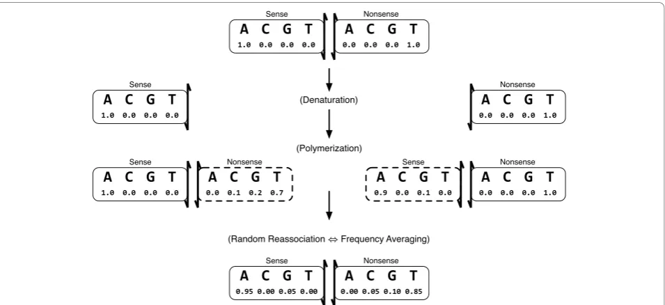
strands are separated and become independent when the DNA is denatured. Taq polymerase proceeds to add stepwise adducts onto each strand in a template-dependent manner. The attachment of a subsequent adduct is independent of the adduct at the previous position. In this way, a newly polymerized nonsense strand is built up using the sense strand as a template. Any mistakes during polymerization result in nucleo-tide mismatches between the strands which are not repaired because Taq polymerase does not contain a proofreading activity nor are other DNA repair enzymes present in the in vitro reaction. The indivi-dual nucleotide site-pairs can thus be considered inde-pendently of all other site-pairs, even though they are physically contiguous with other site-pairs on the oligonucleotide.

Mathematically, this single PCR cycle can be described by an operator Fthat acts on the sense-nonsense pair (s,n) such that

Φ: ( , )s n  1(s Tn), (n Ts) ,

2

1 2

+ +

(

)

where T denotes the Taq polymerase operator (14). Starting from the wild-type sense-nonsense pair (s0,n0)

the probabilistic base-pair mixture after k rounds of

mutagenic PCR can be computed via the iterative for-mula

s nk, k sk ,nk .

(

)

(

)

The resultant sense-strand probability vector sk is

therefore a highly-nonlinear function of theTaq error probabilities. For illustrative purposes we show the ele-gant Pascal-triangle-like hierarchy resulting from explicit representations of {2ksk} fork= 0 ... 7 as follows:

s

Tn s

T s Tn s

T n T s Tn s

T s T n 0

0 0 2

0 0 0

3

0 2 0 0 0

4

0 3 0

2

3 3

4 6

{ }

{ }

{

}

{

}

+ + +

+ + +

+ + TT s Tn s T n T s T n T s Tn s

T s T n

2

0 0 0

5

0 40 3 0 2 0 0 0

6

0 5

4

5 10 10 5

6

+ +

+ + + + +

+

{

}

{

}

0

0 4 0 3 0 20 0 0

7

0 60 5 0 4 0

15 20 15 6

7 21 35

+ + + + +

+ + + +

{

}

T n T s T n T s 335T n3 0+21T s2 0+7Tn0+s0

{

}

For practical computation, however, equation (16) should be used to avoid excessive underflow and trunca-tion errors.

Figure 5A Model of Mutagenic PCR. A model of a single cycle of mutagenic PCR. Each nucleotide of both sense and nonsense strands are treated as probability four-vectors. The‘state’of a nucleotide is the relative frequency we expect to observe it as eitherA, C, G,orT. The initial wild-type sequence is presumed to be well-defined. An example PCR cycle begins withAandTon the sense and nonsense strand, respectively, that are subsequently separated via denaturation. Error-prone polymerization of new nonsense and sense strands byTaq

Given a polymerase matrix T, the overall multi-cycle mutagenic PCR process can be described by computing

sk under four different conditions, namely the condition

that s0 was precisely one of A, C, G, or T. Let s_k

denote the probability vectorskgiven s0 was precisely

nucleotide ℓ. Then we can describe the action of the multi-cycle mutagenic PCR process on the wild-type sequence by the linear 4 × 4 Markov operator Pas the column-concatenation of the s_k such that

P =[skA sCk skG skT] (17)

where, again, each column sums to one. Given a wild-type nucleotide sense-strand state-vector ws and Taq

error probabilities T, operatorPtransformswsinto ms= Pws, where ms is the probability state-vector for a

mutant sense-strand afterkcycles of mutagenic PCR. Under the null hypothesis of‘no selection’, the likeli-hood of misincorporation counts C given mutation probabilities P(T) is given by the product of the four multinomial distributions

Pr | ( )

, , , ,

{

, , , ,

C P T

M p _j c p _j c p _j c p _j c

j

A j C j G j T j

( )

=

( ) ( ) ( ) ( )

∈



A C G T

A,CC,G,T}

,

∏

where

 M

c

c c c c

kj k

j j j j

=

(

)

⎛

⎝ ⎜ ⎜ ⎜

⎞

⎠ ⎟ ⎟ ⎟

∑

( (

( _A,)! _C,)! _G,)!( _T,)!

and each frequencypijis complicated, nonlinear

func-tion of the misincorporafunc-tion frequencies T. Since the entries of T, not P, are the fundamental parameters of likelihood (18), the standard Dirichlet prior described above is inappropriate. Instead, a corresponding nonin-formative‘objective’prior is derived for it, below.

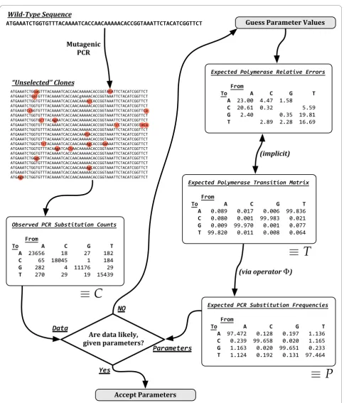
A conceptual flowchart of how parameters T are chosen with respect to counts Cis shown in Figure 6. The figure describes in essence how samples of the posterior Pr(T|C) are realized. It is worth emphasizing that the sixteen parameters of T possess only twelve degrees of freedom, as previously discussed and shown explicitly in Figure 6, because statistical algorithms must be carefully designed to be correct with regard to such constraints.

Polymerase Priors and Posteriors

Choosing a prior distribution for likelihood (18) is not trivial, especially since there is no universal notion of

“complete prior ignorance”[9,37,40]. Choice of prior is therefore governed by specific criteria assumed by the investigator to be important. One nearly universally-accepted criterion is that of reparameterization-invar-iance, a criterion requiring that the inference should not depend on the units of either the parameters or observa-tions. The importance of such invariance has been detailed by Jeffreys [39], Wallace and Freeman [41], Jer-myn [42], and many others. In our context, such invar-iance ensures that parameterizing the likelihood by, for example, either“the expected number of observed mis-incorporations per PCR cycle” or its reciprocal “the expected number of PCR cycles before a misincorpora-tion is observed”yield equivalent inferences. Since there is no meaningful physical difference between these two parameterizations it is essential that each yield equiva-lent results.

Under even highly-mutagenic conditions, the error probabilities given by the columns of T are known a priori to be very close to the extremes of either zero or one. Taq polymerase is one of the best-studied poly-merases in molec