doi:10.5194/tc-4-313-2010
© Author(s) 2010. CC Attribution 3.0 License.
Assessing high altitude glacier thickness, volume and area
changes using field, GIS and remote sensing techniques:
the case of Nevado Coropuna (Peru)
P. Peduzzi1,2, C. Herold1, and W. Silverio3
1United Nations Environment Programme, GRID-Europe, Global Change & Vulnerability Unit, 1219 Chˆatelaine, Switzerland 2Institute of Geomatics and Risk Analysis (IGAR), University of Lausanne, Switzerland
3University of Geneva, Climatic Change and Climate Impacts Research Group, Institute for Environmental Sciences, Switzerland
Received: 6 July 2009 – Published in The Cryosphere Discuss.: 6 October 2009 Revised: 5 August 2010 – Accepted: 6 August 2010 – Published: 23 August 2010
Abstract. Higher temperatures and changes in precipitation patterns have induced an acute decrease in Andean glaciers, thus leading to additional stress on water supply. To adapt to climate changes, local governments need information on the rate of glacier area and volume losses and on current ice thickness. Remote sensing analyses of Coropuna glacier (Peru) delineate an acute glaciated area decline between 1955 and 2008. We tested how volume changes can be estimated with remote sensing and GIS techniques using digital eleva-tion models derived from both topographic maps and satel-lite images. Ice thickness was measured in 2004 using a Ground Penetrating Radar coupled with a Ground Position-ing System durPosition-ing a field expedition. It provided profiles of ice thickness on different slopes, orientations and altitudes. These were used to model the current glacier volume us-ing Geographical Information System and statistical multi-ple regression techniques. The results revealed a significant glacier volume loss; however the uncertainty is higher than the measured volume loss. We also provided an estimate of the remaining volume. The field study provided the scien-tific evidence needed by COPASA, a local Peruvian NGO, and GTZ, the German international cooperation agency, in order to alert local governments and communities and guide them in adopting new climate change adaptation policies.
Correspondence to: P. Peduzzi ([email protected])
1 Introduction 1.1 General context
Changes in glaciers and ice caps are good indicators of cli-mate change (Zemp et al., 2008) and the current trend shows that a majority of the world glaciers have undergone a reduc-tion in their mass at an accelerating rate. The mass loss was greater in the period 1990/91 to 2003/04 than in the previous period 1960/61 to 1989/90 (Bates et al., 2008). This is of concern given that about one-sixth of the world’s population depend on glacier and snow melting for their water supply (Bradley et al., 2006).
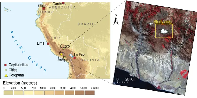
Fig. 1. Location map and study area with 2003 Landsat 7 satellite image (band 2, 3, 4).
1.2 Assessing change of ice volume in Nevado Coropuna, Peru (6500 m a.s.l.)
The present study on the Coropuna Glacier was made at the request of the Cooperaci´on Peruana Alemana de Se-guridad Alimentaria (COPASA) Special Project of Arequipa Regional Government, in collaboration with the Deutsche Gesellschaft f¨ur Technische Zusammenarbeit (GTZ). They asked for scientific-based evidence of glacier area and vol-ume changes, in order to assess whether climate change adaptation policies on water supply should be introduced at local government and communities levels.
The study was carried out by a team from UNEP/GRID-Europe and the University of Geneva. It assessed glacial re-treat using both satellite imagery analysis and in situ mea-surements of the Coropuna Glacier.
This paper describes how glacier area was monitored through time and how to measure the change in volume of the glacier using different Digital Elevation Models (DEMs) as well as evaluate the current (2004) ice thickness. To this end, a field mission was carried out using a Ground Pene-trating Radar (GPR) coupled with a Ground Positioning Sys-tem (GPS). It provided profiles of ice thickness on different slopes, orientations and altitudes. These profiles were used for modelling the entire remaining glacier volume using Ge-ographical Information System (GIS) and statistical multiple regression techniques.
Given the limited financial resources of the local govern-ments and development organisations in Peru, simple and low-cost techniques to measure changes in glacier volume and the remaining ice volume were needed. The purpose of this paper is to test how, with limited budgets and using locally available hardware, scientific evidence of glacier area and volume variation as well as ice thickness can be obtained.
Table 1. Data source for monitoring glaciated area.
Image Acquisition date
Topographic map 1955
Landsat-2 MSS 6 Nov 1980
Landsat-5 TM 12 Jun 1996
Landsat-7 ETM 7 May 2003
ASTER 25 Sep 2008
2 Study area and data sources 2.1 Study area
The Coropuna Glacier is the third highest summit in Peru, culminating at 6446 m. It is located at 15.546◦S, 72.660◦W, about 155 km northwest of the city of Arequipa (Fig. 1). Ac-cording to COPASA staff, 8000 people depend on the Corop-una Glacier for their water supply and it is estimated that 30 000 people depend indirectly on the glacier for their liveli-hoods.
2.2 Data sources
2.2.1 Passive satellite sensors images
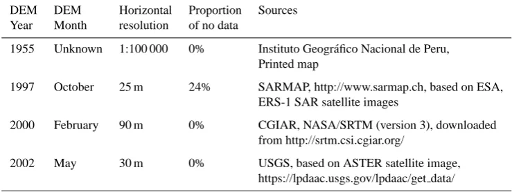
Table 2. Sources and general information for the digital elevation models.
DEM DEM Horizontal Proportion Sources
Year Month resolution of no data
1955 Unknown 1:100 000 0% Instituto Geogr´afico Nacional de Peru,
Printed map
1997 October 25 m 24% SARMAP, http://www.sarmap.ch, based on ESA,
ERS-1 SAR satellite images
2000 February 90 m 0% CGIAR, NASA/SRTM (version 3), downloaded
from http://srtm.csi.cgiar.org/
2002 May 30 m 0% USGS, based on ASTER satellite image,
https://lpdaac.usgs.gov/lpdaac/get data/
2.2.2 Digital elevation models
In order to estimate the ice volume loss between 1955 and 2002, four Digital Elevation Models (DEMs) from different years were considered. Although eight DEMs in total were available for Coropuna, the period of data acquisition was the first criterion considered for selection to ensure adequate time span between datasets. The quality of the dataset was the second criterion. Four DEMs were thus selected from the following years: 1955, 1997, 2000 and 2002.
The DEM 1955 was generated by manually digitising the elevation contour lines from the topographic map of 1955. The DEM 1997 was purchased from the company SARMAP which produced it based on a pair of ERS-1 Syn-thetic Aperture Radar (SAR), a satellite from the European Space Agency. The DEM 2000 was based on radar mea-surements from the NASA Shuttle Radar Topographic Mis-sion (SRTM, verMis-sion 3). The DEM 2002 was derived from ASTER satellite data, DEM provided by United States Geo-logical Survey (USGS) (see Table 2).
2.2.3 Field measurements
The purpose of the expedition was to measure the depth of the ice as well as taking GPS points for the adjustment of the DEMs. The 14 day-mission was undertaken between 13 and 26 August 2004. The team was composed of two scientists and 11 support staff.
The scientific instruments were chosen based on local availability (as opposed to most efficient). The GPR Ramac X3M included a 100 MHz shielded antennas. Much lighter GPR exist; however, it was the only GPR available in Are-quipa. Three Global Positioning System receptors (GPS) and two regular office laptops for controlling the GPR unit and recording the data were used. Due to the limitations of the computer’s hard disk at low pressure conditions (the read-ing heads would touch the disks and damage them), hard disks were removed. Computers and software were booted on CDs, and measurements were recorded on USB cards.
3 Methodology
3.1 Estimation of ice thickness
Measuring the ice thickness was achieved using the GPR, with a sampling frequency of 438 MHz. Technical settings are specified in Table 3. The signal was assumed to travel through ice at 0.16 m/ns±0.01 m/ns according to other stud-ies performed in similar conditions (Gruber, Ludwig and Moore, 1996; Moorman and Michel, 2000; Descloitres et al., 1999). The depth of ice can be measured by recording the time lag between the emission and the reception of the signal (see Eq. 1)
I=T C
2 (1)
Where I= Ice thickness [m], T= Time [ns], C= Speed of propagation through ice of the signal (0.16 [m/ns]) For ex-ample a time lag of 2000 ns = 160 m of ice thickness.
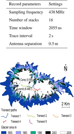
Each recorded depth was coupled with geographical coor-dinates obtained by a GPS so that the profiles could be geo-referenced and speed of radar over ground computed (given that for each GPS location, the time is also recorded). Due to time and access constraints, it was not possible to achieve a comprehensive coverage of the glaciated area. Instead, the mission proceeded along transects (shown on Fig. 2). The selected transects were chosen to provide samples includ-ing different altitudes, slopes, and aspects (slope orientation). We proposed (and tested) the hypothesis that these three vari-ables would explain most of the ice thickness. Using multi-ple regression analysis, depth was modelled in areas where no measurements were taken.
Table 3. GPR settings.
Record parameters Settings
Sampling frequency 438 MHz
Number of stacks 16
Time window 2055 ns
Trace interval 2 s
Antenna separation 0.5 m
Fig. 2. Georeferenced radar profiles and evolution of glaciated area
(1955–2008).
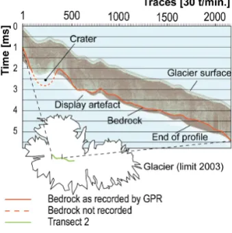
“Kingdom Suite” to estimate ice depth. Due to the com-puter configuration that limited recording time windows, the bedrock was sometimes too deep to be detected (typically in volcanic craters, see Fig. 9). However, as an approximation, profiles can be extrapolated by following ice stratification. 3.2 Estimation of ice volume loss
Although passive satellite sensors, such as Landsat TM, pro-vide an estimate of the area covered by ice (see Sect. 4.1) passive sensors do not provide information on the changes in ice thickness. However, the difference of ice volume may be estimated by using DEM time series.
3.2.1 Adjustment and corrections
In order to compare the different DEMs, several operations were needed. Firstly, all the DEMs were re-sampled to 30 m to compensate for different spatial resolutions. They were then reprojected in Universal Transverse Mercator (UTM), projection 18 south, datum WGS84. Finally, they were geo-referenced so that they could be overlaid. This was per-formed using 32 control points, such as summits located out-side the glacier area (on bare rocks).
Previous studies highlighted the issue of DEMs such as ASTER or SRTM which appear to have a bias following altitude (Berthier et al., 2004) or reveal significant errors when applied to rugged terrain and steep slopes (K¨a¨ab et al., 2002). In all DEMs, a reference area was chosen on surfaces that were not covered by ice, snow or vegetation (i.e. rocky or bare ground). This corresponds to the area outside the glaciated area of 1955. A sample of 1009 points located on an ellipse outside the glaciated areas was used to extract in-formation on easting(X), northing(Y ), elevation, slope and aspect (slope orientation). These factors proved to influence the DEM errors in other studies (Gorokhovich and Voustian-iouk, 2006). To verify whether the DEMs used were well-adjusted, the differences in altitude were computed against the reference area (DEM 2000–DEM 1955; DEM 1997– DEM 1955 and DEM 2002–DEM 1955).
Then the differences between DEMs were plotted in 3-D along withX andY. Despite the fact that the DEMs are all in the same geographic projection, Fig. 3 shows that they are not in the same plan, with DEM 1997 having the least distor-tions and DEM 2002 (ASTER) showing the worst distortion. If the DEMs are not in the same plan, a change in latitude and longitude can significantly influence the difference in el-evation
This can be corrected using the following linear regression (see Eq. 2):
DEMt=DEM−aX+bY+c) (2)
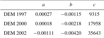
Where DEMt is the new values corrected for theX andY. The weightsa,b,cused to correct the DEMs are provided in Table 4.
After this first correction, there were still some bias in-duced by aspect and elevation. To correct these, a quadratic equation was applied. The aspect variable was transformed by taking the cosine of the angle (expressed in radians).This is necessary as an orientation of 359◦is close to an orienta-tion of 1◦.
This distortion from elevation and aspect was corrected us-ing Eq. (3):
DEMt2=DEMt−(aEl+bcos(As)+cEl·cos(As)+dEl2 +e (cos(As))2+f ) (3) Where: DEMt2 = DEMt further corrected with elevations and cosine of the aspects El = Elevation As = Aspect (slope orientation)
Fig. 3. Difference between DEMs plotted alongXandY.
Fig. 4. Difference on rocky areas versus elevation and aspect for ASTER 2002.
Table 4. Weights used to place the DEMs in the same plan as DEM
1955.
a b c
DEM 1997 0.00027 −0.00115 9315
DEM 2000 0.00018 −0.00218 17958
DEM 2002 −0.00111 −0.00420 35643
Table 5 shows that for the ASTER DEM it was possible to reduce the error by almost two thirds (from 42.1 to 14.4), although there was still an off-set of 3.28. The standard devi-ation (STDEV) and average difference are computed over all the rocky areas higher than 4400 m (i.e. 533 689 pixels). Er-rors calculated on exposed rock are not necessarily fully rep-resentative of the potential systematic errors on the glaciated terrain.
While this study was carried out in 2004–2005, a parallel study was ongoing using a similar approach on Coropuna, of which we were informed later (Racoviteanu et al., 2007). They built a DEM based on a topographic map of 1955, but at a more precise scale of 1:50 000. They used DEM from ASTER 2001 and SRTM 2000 datasets. Although the ini-tial approach is similar (with exception that we used an ad-ditional DEM from 1997 and the ASTER 2002), there are several significant differences in the results of the two stud-ies:
Racoviteanu et al. succeeded to bring the standard devia-tion on rocky area to 9.5 m for SRTM (DEM 2000) as com-pared to 13.2 m in our study. This might be explained by the use of a more precise map (1:50 000 as compared to our 1:100 000), but could also be due to a smaller sample of ref-erence points to compute the standard deviation (61 points in their study as compared with 533 689 in our present study for rocky areas).
Table 5. Assessing the DEMs accuracy before and after corrections (on rocky areas).
Original image Correction 1 (X&Y) Correction 2 (El & As)
Difference STDEV Difference STDEV Difference STDEV
DEM97-55 −0.24 m 18.6 −0.24 m 16.1 0.00 18.6
DEM00-55 0.04 m 18.2 0.00 m 13.2 0.00 13.2
Dem02-55 71.01 m 42.1 2.71 m 27.9 3.28 14.4
Fig. 5. ASTER 2008 image (band 1, 2, 3).
4 Results
4.1 Change in ice cover
The identification of ice cover using images from passive satellite sensors is very straightforward in this location. As long as images are selected outside the snowy season (i.e. not between December and April), the ice detection is facilitated by the high contrast between the dark volcanic rock and the ice. The summits have a smooth shape, thus without much shadows (see Fig. 5). The images were projected in UTM 18S (datum WGS84), they were georeferenced, classified. The classes corresponding to ice cover were transformed into vectors and the area computed using GIS.
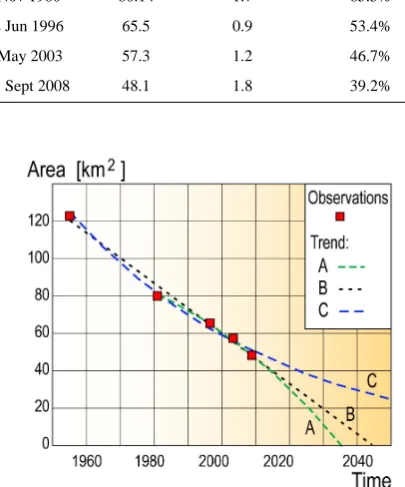
The map in Fig. 2 shows the ice cover changes for the five dates. This first analysis revealed that the Coropuna Glacier shrunk steadily from 122.7 Km2in 1955 to 48.1 km2in 2008, i.e. losing more than 60% of its surface in 53 years (Table 6). By plotting glacier area through time (Fig. 6) a clear de-clining trend appears. However with these observations it is not possible to predict whereas this will follow an accelerat-ing trend (A) correspondaccelerat-ing to smaller volume of ice havaccelerat-ing less inertia, thus shrinking faster. A linear trend (B), or a decelerating trend (C), where the shrinking will be slower when affecting higher altitudes. While scenarios A and B do not make much difference (total decline around 2040), in the
Table 6. Evolution of ice cover.
Date Glacier Ice area Remaining ice cover surface (km2) loss (km2/y) (1955 as reference)
1955 122.7 100%
6 Nov 1980 80.14 1.7 65.3%
12 Jun 1996 65.5 0.9 53.4%
7 May 2003 57.3 1.2 46.7%
25 Sept 2008 48.1 1.8 39.2%
Fig. 6. Glacier areas through time and different scenarios.
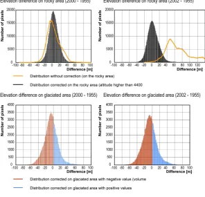
Fig. 7. Elevation differences on rock and on glaciated areas.
4.2 Ice volume loss
Except the DEM 1997 (of which 24% did not contain data especially with respect to glaciated area), both SRTM 2000 and ASTER 2002 provide similar elevation differences. Ac-cording to these results the average elevation changes were −8.75±13.2 m (DEM 2000) and −9.4m±14.4 m (DEM 2002) at 95% confidence interval (see Table 7 for values and Table 5 for the margin of error). This corresponds to a yearly average loss of about−0.2m±0.3 m per year (at 95% confi-dence interval). Once extrapolated to the volume, the loss of ice between 2002 and 1955 is estimated to be 1.2 km3. This corresponds to an ice volume decrease of 18% as compared with 1955. These figures should be taken with caution given the low accuracy of the DEM, as illustrated by the measured difference being lower than the margin of error.
Unfortunately the DEM 1997 includes numerous pixels without data, especially on glaciated areas, making it less reliable. Figure 7 shows the significant improvements (es-pecially on ASTER DEM) that can be achieved after cor-rection of the DEMs. The margin of errors (see Table 5) is still higher than the measured differences (see Table 7), but this error follows a normal distribution with a clear higher amount of pixels depicting a decrease in elevation change (see Fig. 7).
Table 7. Altitude changes on glaciated areas on original and corrected images.
DEM97-55 DEM00-55 Dem02-55
Original DEMs −1.35 m −5.05 m + 28.85 m
DEMs corrected −3.36 m −8.75 m −9.40 m∗
∗Once the off-set of 3.28 is removed, otherwised the average difference on ice is
−6.11.
The much smaller differences observed in 1997 as com-pared with 2000 and 2002 are more likely due to data quality rather than linked with a 6 m decrease in ice thickness be-tween 1997 and 2002.
Fig. 8. Estimation of ice loss between 1955 and 2000 and between
1955 and 1997.
4.3 Remaining ice
4.3.1 Analysing the transects
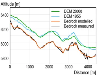
Figure 9 shows a portion (about 50%) of transect 2. This part is interesting as it shows that in some areas, the bedrock (in orange) is too deep to be recorded (see in the Crater). 4.3.2 Modelling remaining ice: results
In order to extrapolate the estimation of the ice volume to the rest of the map, the hypothesis was made that the depth of ice was dependent on the altitude, the aspect (slope’s orientation) and the slopes. The assumption was made that ice thickness would depend on these three components. The amount of precipitation should be driven by altitude, slope and orienta-tion. Orientation should also play a role due to predominant wind direction as well as different solar exposure (also prob-ably less prominent in the tropics). Finally, snow accumula-tion should also be driven by slopes, based on the hypothesis that on steep slopes the ice should be thinner as the glacier is
Fig. 9. Example of interpreted profile of transect 2 from the GPR
on the slope to the summit.
moving faster, whereas on gentle slopes, the ice accumulates as the glacier slows down.
To test these hypotheses, a statistical multiple regressions analysis was made using the recorded depth in relation to altitude, slope and orientation.
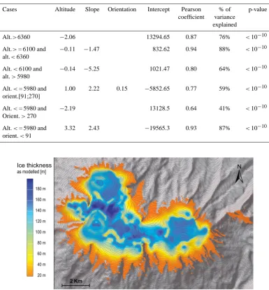
It was necessary to differentiate six cases (see Table 8): the top of volcanoes with altitudes higher than 6360 m; areas with altitudes between 6100 and 6360 m; and altitudes be-tween 5980 and 6100 m. The next categories used three dif-ferentiations of slope orientation. These were needed for al-titudes lower than 5980 m with the following aspects: higher than 270◦, between 91◦and 270◦and smaller than 91◦. Ta-ble 8 describes the variaTa-bles (altitude, slope and orientation) and weight (in bold) used in the model according to the dif-ferent thresholds. The quality of the models was assessed by looking at p-value1(all smaller than 10−10)and Pearson coefficient (between 0.80 and 0.94 for altitudes higher than 5980 m). The model becomes less accurate for lower eleva-tions, which is reflected by a lower correlation (between 0.64 and 0.77 except one at 0.93).
Equations from Table 8 suggest that except for case 4 where orientation of slopes seems to play a role, in all the other cases, the depth of ice can be explained by altitude and slopes only. At the summit (altitude>6360 m) ice depth is only linked with altitude. This is not surprising given that the smooth round summits of Coropuna are mostly flat (hence limited slopes and orientation). The map in Fig. 10 shows the result of this model once extrapolated to the entire glacier.
The modelled thickness ranges between 20 and 200 m, with an average thickness estimated at 80.8 m±16.5 m (at 95% confidence interval). This gives an expected remaining ice volume of 4.62 km3 (±20.3%). The margin or error is 1In broad terms, a p-value smaller than 0.05, shows the
Table 8. Quality of regressions used for modelling ice thickness.
Cases Altitude Slope Orientation Intercept Pearson % of p-value
coefficient variance explained
Alt.>6360 −2.06 13294.65 0.87 76% <10−10
Alt.>= 6100 and −0.11 −1.47 832.62 0.94 88% <10−10
alt.<6360
Alt.<6100 and −0.14 −5.25 1021.47 0.80 64% <10−10
alt.>5980
Alt.<= 5980 and 1.00 2.22 0.15 −5852.65 0.77 59% <10−10
orient.[91;270]
Alt.<= 5980 and −2.19 13128.5 0.64 41% <10−10
Orient.>270
Alt.<= 5980 and 3.32 2.43 −19565.3 0.93 87% <10−10
orient.<91
Fig. 10. Estimation of ice thickness (model).
fairly important at±0.94 km3; however, this result only pro-vides a rough estimate.
The multiple regression analysis confirmed that altitude, slopes and orientation are factors influencing the ice thick-ness. This illustration includes transect 2, 3 and 4 (see Fig. 2 for their locations), thus offering the longest stretch across the measurements. The modelled depth fits well with the recorded profiles. The Pearson correlation between ice depths measured and modelled is 0.87 with a standard de-viation of 16.5 (at 95% confidence interval). Figure 11 pro-vides the fit between the observed and modelled depths. Still, for obvious reason of access, we were not able to take mea-surements on steep slopes with the GPR. This lack of sam-ples might have an effect on the model. The maximum ice thickness on steep slopes, especially below the west summit,
might be a limitation of our model to capture these physical conditions. The DEM 2000 shows an increase in elevation in higher than 6160 (areas where the green line above the blue line in Fig. 11). Elevation loss can be seen on lower summits (area where blue line is below green line in Fig. 11).
5 Discussion
5.1 Estimation of the evolution in ice cover
Fig. 11. Ice thickness measured vs. modelled (transects 2, 3 and 4).
say whereas the projected decline will be abrupt or slow. It is possible that with a new estimation in year 2015, the trend might be better identified.
5.2 Measuring ice thickness
The hypothesis made on the statistical link between altitude, slope and orientation proved to be successful, except for ori-entation, which plays a limited role (mostly non-significant except in one case). It was expected that orientation would play a bigger role due to direction of the predominant wind, precipitation coming mostly from one direction. The limited role played by orientation is probably due to the study area’s location within the tropics where the sun is less predomi-nant on a specific slope (such as south in northern latitudes or north in southern latitudes). For glaciers at higher (North-ern Hemisphere) or lower (South(North-ern Hemisphere) latitudes, slope orientation might play a bigger role and should not be disregarded in the model.
5.3 Limitations on measuring the difference in ice volume
In this analysis, the differences recorded on the rocky ar-eas were significant and raised concerns on the ability to use DEMs. In any case, they could not be used without the ad-justments. The corrections applied on easting and northing as well as on elevation and aspects (for DEM 2002) signifi-cantly improved the quality of the DEMs. The Radar DEM 1997 included numerous no-data. Another limitation lies in the fact that digital DEMs are fairly recent technologies, and the date of the oldest archive found for the Coropuna was 1997.
The methodology for identifying the ice volume loss using DEM is straightforward and less challenging compared to the estimation of remaining ice. The difficulty comes from the lack of precision of DEMs on rough terrain, and attempts to correct the distortions can be time- consuming.
6 Conclusions and perspectives
The simple computation of area decrease based on passive satellite sensors, show a rapid decline of Glacier Coropuna (−1.4 km2per year,−60% since 1955) and if this continues, it may be gone before 2045. This is why it was important to try to produce more complex evaluations in terms of volume loss and remaining ice.
The methodology chosen for ice thickness and ice volume loss estimation proved to be effective. The corrections ap-plied on the DEMs through multiple regression models based on easting, northing, aspect and elevation reduced the uncer-tainties, although the margin of errors is still high.
The vertical accuracy for the differences computed be-tween the DEM2000t, the DEM2002t and the DEM 1955 were estimated at±13.2 and 14.4 m respectively, for eleva-tion changes of−8.75 and−9.4 m on the ice (i.e. an average of 0.19 to 0.2 m of decrease per year,±0.3 m). Errors calcu-lated on exposed rock are not necessarily fully representative of the potential systematic errors on the glaciated terrain. Al-though this provides an estimate of ice loss trends, the differ-ence in ice thickness is smaller than the margin or error, thus affecting the confidence in the measurements. This can only be improved by either satellite sensors with better precision or by pursuing research in finding methods for correcting the DEMs.
For the ice thickness, the methodology could be improved, notably by choosing a lighter GPR. This would have eased the data collection, for instance by using skis to cover a much bigger area. Using the profiles from the ground study and a statistical extrapolation (modelling), it was possible to esti-mate the ice thickness (in average 80.8 m±16.5 m), which gives an estimated remaining volume of 4.62 km3±0.94km3 (i.e. 3.2 million tonnes of water).
These results were presented to GTZ and COPASA in Are-quipa in December 2005. It helped to raise awareness on the issue of shrinking glaciers. In 2006, COPASA obtained support from GTZ. We then presented our results to United Nations Development Programme (UNDP) and they agreed to support COPASA through their Global Risk Information Programme (GRIP). Later on, the Inter-American Develop-ment Bank (IADB) also joined. These institutions help to introduce new policies for climate change adaptation at both local government and community levels: between 2006 and 2009, the following actions were carried out:
and are working on climate change topic; the issue has been brought to the attention of regional institutions, which then produced a regional strategy for climate change adaptation. Three university theses have studied climate change at the re-gional level; four educational brochures were developed and their use approved in primary and secondary schools; a board game was developed on Climate Change Adaptation to help children to learn while playing. Five mini reservoirs and 15 warehouses for forage were built in this area.
The recent 2008 ASTER image shows that the glacier area continues to shrink, however, the local authorities have now integrated this threat into their development plan. The threat on water supply might be increasing, but efforts are made to reduce the vulnerability of the local population.
Acknowledgements. This work was supported by the GTZ/COPASA, Arequipa. We would like to thank Josef Haider, Juan Carlos Montero and all the team of GTZ/COPASA in Arequipa for the logistical support and for trusting us in conducting this study. We also would like to thank Carlos Zarate and all his team of guides, porters, cook, and drivers for the expedition on Coropuna, and the team of Peruvian Geophysical Institute in Arequipa. Without all this combined support, this research would not have been possible. For the help provided on seismic and GPR data acquisition and analysis, we would like to thank Milan Beres, Julien Fiore and Micha¨el Fuchs of the Department of Geology, University of Geneva; Jacques Jenny of Geo2x; Franc¸ois Marillier and Dieb Hammami of Geophysical Institute, University of Lausanne; and Ansgar Forsgren of Mala Geoscience. We also would like to thank Marisol Estrella and John Harding for kindly reviewing the English.
Edited by: G. H. Gudmundsson
References
Bates, B. C., Kundzewicz, Z. W., Wu, S., and Palutikof, J. P.: Climate Change and Water, Technical Paper of the Intergov-ernmental Panel on Climate Change, IPCC Secretariat, Geneva, 210 pp., available at: http://www.ipcc.ch/pdf/technical-papers/ climate-change-water-en.pdf (last access: August 2010), 2008. Barenett, T. P., Adam, J. C., and Lettenmaier, D. P.: Potential
impacts of a warming climate on water availability in snow-dominated regions, Nature, 438, 303–309, 2005.
Berthier, E., Arnaud, Y., Baratoux, D., Vincent, C., and R´emy, F.: Recent rapid thinning of the “Mer de Glace” glacier derived from satellite optical images, Geophys. Res. Lett., 31, 1–4, 2004. Bradley, R. S., Vuille, M., Diaz, H. F., and Vergara, W.: Threats to
water supplies in the tropical Andes, Science, 312, 1755–1756, 2006.
Descloitres, M., Gu´erin, R., Ramirez, E., Gallaire, R., Ribstein, P., and Valla, F.: D´etermination de l’´epaisseur des glaciers de Sarenne (Alpes) et de Chacaltaya (bolivie) par prospection radar au sol `a 50 MHz, La Houille Blanche 5, 29–33, 1999.
Eisen, O., Nixdorf, U., Keck, L., and Wagenbach, D.: Alpine ice cores and ground penetrating radar: combined investigations for glaciological and climatic interpretations of a cold Alpine ice body, Alfred-Wegener-Institut f¨ur Polar- und Meeresforschung
Bremerhaven, Institut f¨ur Umweltphysik, Universit¨at Heidel-berg, 2003.
Gorokhovich, Y. and Voustianiouk, A.: Accuracy assessment of the processed SRTM-based elevation data by CGIAR using field data from USA and Thailand and its relation to the terrain character-istics, Remote Sens. Environ., 104, 409–415, 2006.
Gruber, S., Ludwig, F., and Moore, J. C.: Application of Ground Penetrating Radar in Glaciology and Permafrost Prospecting, Geographisches Institut/JLU Gießen, 1996.
K¨a¨ab, A., Huggel, C., Paul, F., Wessels, R., Raup, B., Kiefer, H., and Kargel, J.: Glacier Monitoring from ASTER imagery: accuracy and applications, Proceedings of EARSeL-LISSIG-Workshop Observing our Cryosphere from Space, Bern, Switzer-land, 2002.
Liu, Y.: An evaluation of the data quality of SRTM DEM at the alpine and plateau area, north-western of China, The Interna-tional Archives of the Photogrammetry, ISPRS, 37(Part B1), 1123–1128, 2008.
Maijala, P., Moore, J. C., Hjelt, S.-E., P¨alli, A., and Sin-isalo, A.: GPR Investigations of Glaciers and Sea Ice in the Scandinavian Arctic, GPR98 – 7th International Con-ference on Ground-Penetrating Radar Proceedings, 143–148, available at: http://kaares.ulapland.fi/home/hkunta/jmoore/pdfs/ maijalagpr98.pdf (last access: August 2010), 1998.
Moorman, B. J. and Michel, F. A.: Glacial hydrological system characterization using ground-penetrating radar, Hydrol. Pro-cess., 14, 2645–2667, 2000.
NASA, SRTM mission statistics, available at: http://www2.jpl.nasa. gov/srtm/statistics.html, last access: August 2010.
Rabus, B., Eineder, M., Roth, A., and Bamler, R.: The shuttle radar topography mission – a new class of digital elevation models ac-quired by spaceborne radar, Photogramm. Rem. Sens., 57, 241– 262, 2003.
Racoviteanu, A. E., Manley, W. F., Arnaud, Y., and Williams, M. W.: Evaluating digital elevation models for glaciologic appli-cations: An example from Nevado Coropuna, Peruvian Andes, Global Planet. Change, 59, 110–125, 2007.
S´en´echal, G., Rousset, D., Salom´e, A.-L., and Grasso, J.-R.: Geo-radar and seismic investigations over the Glacier de la Girose (French Alps), Laboratoire d’imagerie g´eophysique, Universit´e de Pau, Laboratoire de g´eophysique interne et tectonophysique, Universit´e Joseph Fourier, Grenoble (France), 2005.
Silverio, W. and Jaquet, J.-M.: Glacial cover mapping (1987–1996) of the Cordillera Blanca (Peru) using satellite imagery, Remote Sens. Environ., 342–350, 2005.
Vimeux, F., Ginot, P., Schwikowski, M., Vuille, M., Hoffmann, G., Thompson, L. G., and Schottererg, U.: Climate variability during the last 1000 years inferred from Andean ice cores: A review of methodology and recent results, Palaeogeogr. Palaeocl., 281(3– 4), 229–241, 2009.
Vuille, M., Francou, B., Wagnon P., Juen, I., Kaser, G., Bryan G. M., and Bradley, R. S.: Climate change and tropical Andean glaciers: Past, present and future, Earth-Sci. Rev., 89, 79–96, 2008.