www.the-cryosphere.net/1/41/2007/ © Author(s) 2007. This work is licensed under a Creative Commons License.
The Cryosphere
Using in-situ temperature measurements to estimate saturated soil
thermal properties by solving a sequence of optimization problems
D. J. Nicolsky1, V. E. Romanovsky1, and G. S. Tipenko2
1Geophysical Institute, University of Alaska Fairbanks, PO Box 757320, Fairbanks, AK 99775, USA
2Institute of Environmental Geoscience Russian Academy of Sciences, 13-2 Ulansky pereulok, PO Box 145, Moscow, Russia
Received: 1 August 2007 – Published in The Cryosphere Discuss.: 9 August 2007
Revised: 17 October 2007 – Accepted: 6 November 2007 – Published: 22 November 2007
Abstract. We describe an approach to find an initial approx-imation to the thermal properties of soil horizons. This tech-nique approximates thermal conductivity, porosity, unfrozen water content curves in horizons where no direct temperature measurements are available. To determine physical prop-erties of ground material, optimization-based inverse tech-niques are employed to fit the simulated temperatures to the measured ones. Two major ingredients of these techniques are an algorithm to compute the soil temperature dynamics and a procedure to find an initial approximation to the ground properties. In this article we show how to determine the ini-tial approximation to the physical properties and present a new finite element discretization of the heat equation with phase change to calculate the temperature dynamics in soil. We successfully apply the proposed algorithm to recover the soil properties for the Happy Valley site in Alaska using one-year temperature dynamics. The determined initial approxi-mation is utilized to simulate the temperature dynamics over several consecutive years; the difference between simulated and measured temperatures lies within uncertainties of mea-surements.
1 Introduction
Recently, the Arctic Climate Impact Assessment report (ACIA, 2004) concluded that climate change is likely to sig-nificantly transform present natural environments, particu-larly across extensive areas in the Arctic and sub-Arctic. Among the highlighted potential transformations is soil warming which can potentially cause an increase in the ac-tive layer thickness and degradation of permafrost as well as have broader impacts on soil hydrology, northern ecosystems and infrastructure. Since permafrost is widely distributed and Correspondence to: D. J. Nicolsky
covers approximately 25% of the land surface in the Northern Hemisphere (Brown et al., 1997), it is very important to un-derstand the causes affecting soil temperature regime. One approach to studying soil temperature dynamics and their dependence on climate variability is to employ mathemat-ical modeling (Goodrich, 1982; Nelson and Outcalt, 1987; Kane et al., 1991; Zhuang et al., 2001; Ling and Zhang, 2003; Oleson et al., 2004; Sazonova et al., 2004; M¨olders and Ro-manovsky, 2006)
A mathematical model of soil freezing/thawing is based on finding a solution of a non-linear heat equation over a speci-fied domain, (see Andersland and Anderson, 1978; Yershov, 1998, and many references therein). The domain represents ground material and is divided into several horizons (e.g. an organic matt, an organically enriched mineral soil layer, and a mineral soil layer) each with its distinct properties charac-terized by mineral-chemical composition, texture, porosity, heat capacity and thermal conductivity. By parameterizing the coefficients in the heat equation within each horizon, it is possible to take into account temperature-dependent latent heat effects occurring when ground freezes and thaws. This approach yields a realistic model of temperature dynamics in soils. However, in order to produce quantitatively reason-able results, it is necessary to prescribe physical properties of each horizon.
Roth, 1997; Yoshikawa et al., 2004). More accurate mea-surements of the total water content (ice and water together) can be acquired by thermalization of neutrons and gamma ray attenuation. This is not always suitable for Arctic re-gions as it requires transportation of radioactive equipment to remote locations (Boike and Roth, 1997). An alternative to the above-mentioned methods and also to a number of others (Schmugge et al., 1980; Tice et al., 1982; Ulaby et al., 1982; Stafford, 1988; Smith and Tice, 1988) is the use of inverse modeling techniques. These techniques estimate the water content and other thermal properties of soil using in-situ tem-perature measurements and by exploiting the mathematical model.
A variety of inverse modeling techniques that recover the thermal properties of soil are known. Many of them rely on the commonly called source methods (Jaeger and Sass, 1964), in which temperature response due to heating is mea-sured at a certain distance from the heat source. The temper-ature response and geometry of the probe are used to com-pute the thermal properties by either direct or indirect meth-ods. In the direct methods, the temperature measurements are explicitly used to evaluate the thermal properties. In the indirect methods, one minimizes a discrepancy between the measured and the synthetic temperatures, the latter computed mathematically by exploiting the heat equation in which the coefficients are parameterized according to the specified ther-mal properties.
Application of direct methods such as the Simple Fourier Methods (Carson, 1963), Perturbed Fourier Method (Hur-ley and Wiltshire, 1993), and the Graphical Finite Difference Method (McGaw et al., 1978; Zhang and Osterkamp, 1995; Hinkel, 1997) yield accurate results for the thermal diffusiv-ity (the ratio of the thermal conductivdiffusiv-ity and the heat capac-ity), only when water does not undergo the phase change. Despite the fact that the direct methods are well established for the heat equation without the phase change, no univer-sal framework exists in the case of the soil freezing/thawing because the heat capacity and thermal conductivity depend strongly on the temperature in this case.
A common implementation of the indirect methods uses an analytical or numerical solution of the heat equation to eval-uate the synthetic temperature. Due to strong non-linearities, the analytical solution of the heat equation is known only for a limited number of cases (Gupta, 2003), whereas nu-merical solutions are typically computable. Given a nu-merical solution computed by finite difference (Samarskii and Vabishchevich, 1996) or finite element (Zienkiewicz and Taylor, 1991) methods, one can minimize a cost function,J, which measures a discrepancy between the measuredTmand syntheticTctemperatures. The typical expression for the cost function,J, is given by
J (C)≈
Z te
ts
(Tm(xi, t )−Tc(xi, t;C))2dt. (1)
Here, the quantityCis the control vector that is a set of pa-rameters defining soil properties of each soil horizon. The synthetic temperature,Tc, is computed by the mathematical model parameterized by variables inCat some depthsxiover the time interval[ts, te].
In this article, we deal with optimization techniques that find soil properties by minimizing the cost function (1). Commonly, the cost functionJis minimized iteratively start-ing from an initial approximation C0 to the parameters C (Thacker and Long, 1988). Since the heat equation is non-linear, in general there are several local minima. Hence, it is important that the initial approximation lies in the basin of attraction of a proper minimum (Avriel, 2003).
We present a semi-heuristic algorithm to determine an ini-tial approximation C0, for use as the starting point in mul-tivariate minimization of cost functions such as (1). In this article, we use in-situ measured temperatureTmto formulate the cost functionJ. We construct the initial approximation by minimizing cost functions over specifically selected time intervals[ts, te]in a certain order. For example, first, we pro-pose to find thermal conductivity of the frozen soil using the temperature collected during winter, and then use these val-ues to find properties of the thawed soil. In order to minimize the cost function it is necessary to compute the temperature dynamics multiple times for various control vectorsC. Since an analytical solution of the non-linear heat equation is not generally available, we use a finite element method to find its solution. To compute latent heat effects, we propose a new fixed grid technique to evaluate the latent heat terms in the mass (compliance) matrix using enthalpy formulation. Our techniques do not rely on temporal or spatial averaging of enthalpy, but rather evaluate integrals directly by employing a certain change of variables. An advantage of this approach is that it reduces the numerical oscillation of the temperature dynamics at locations near 0◦Cisotherm.
The structure of this article is as follows. In Sect. 2, we describe a commonly used mathematical model of tempera-ture changes in the active layer and near surface permafrost. In Sect. 3, we outline a finite element discretization of the heat equation with phase change. In Sect. 4, we introduce main definitions, notations and state the variational approach to find the thermal properties. In Sect. 5, we provide an algo-rithm to construct an initial approximation to thermal proper-ties. In Sect. 6, we apply our method to estimate the thermal properties and the coefficients determining the unfrozen wa-ter content at a site located in Alaska. In Sect. 7, we state limitations and shortcomings of the proposed algorithm. Fi-nally, in Sect. 8, we provide conclusions and describe main results.
2 Modeling of soil freezing and thawing
be simulated by a 1-D heat equation with phase change (Carslaw and Jaeger, 1959):
C∂
∂tT (x, t )+L ∂
∂tθl(T , x)= ∂ ∂xλ
∂
∂xT (x, t ), (2)
where x∈[0, l], t∈[0, τ]; the quantities C=C(T , x)
[Jm−3K−1]andλ=λ(T , x)[Wm−1K−1] stand for the volu-metric heat capacity and thermal conductivity of soil, respec-tively; L [Jm−3] is the volumetric latent heat of fusion of water, andθlis the volumetric liquid water content. We note that this equation is applicable when migration of water is negligible, there are no internal sources or sinks of heat, frost heave is insignificant, and there are no changes in topography and soil properties in lateral directions. Typically, the heat Eq. (2) is supplemented by Dirichlet, Neumann, or Robin boundary conditions specified at the ground surface, x=0, and at the depthl(Carslaw and Jaeger, 1959). In geothermal studies, a Neumann boundary condition is typically set at the depthl. In this study we use the measured temperaturesTu andTlto set the Dirichlet boundary conditions at depthsx=0 andx=l, respectively, i.e.T (0, t )=Tu(t ),T (l, t )=Tl(t ). In order to calculate the temperature dynamicsT (x, t ) at any timet∈[0, τ], Eq. (2) is supplemented by an initial condi-tion, i.e. T (x,0)=T0(x), whereT0(x)is the temperature at x∈[0, l]at timet=0.
In certain conditions such as waterlogged Arctic lowlands, soil can be considered a porous media fully saturated with water. The fully saturated soil is a multi-component sys-tem consisting of soil particles, liquid water, and ice. It is known that the energy of the multi-component system is min-imized when a thin film of liquid water (at temperature below 0◦C) separates ice from the soil particles (Hobbs, 1974). A film thickness depends on soil temperature, pressure, miner-alogy, solute concentration and other factors (Hobbs, 1974). One of the commonly used measures of liquid water below freezing temperature is the volumetric unfrozen water con-tent (Williams, 1967; Anderson and Morgenstern, 1973; Os-terkamp and Romanovsky, 1997; Watanabe and Mizoguchi, 2002). It is defined as the ratio of liquid water volume in a representative soil domain at temperatureT to the volume of this representative domain and is denoted byθl(T ). There are many approximations to θl in the fully saturated soil (Lunardini, 1987; Galushkin, 1997). The most common ap-proximations are associated with power or exponential func-tions. Based on our positive experience in (Romanovsky and Osterkamp, 2000), we parameterizeθl by a power function
θl(T )=a|T|−b;a, b>0 forT <T∗<0◦C (Lovell, 1957). The
constantT∗ is called the freezing point depression (Hobbs,
1974), and from the physical point of view it means that ice does not exist in the soil ifT >T∗. In thawed soils (T >T∗),
the amount of water in the saturated soil is equal to the soil porosityη, and hence the functionθl(T )can be extended to
T >T∗asθl(T )=η. Therefore, we assume that
θl(T , x)=η(x)φ (T , x), φ=
1, T ≥T∗
|T∗|b|T|−b, T < T∗
, (3)
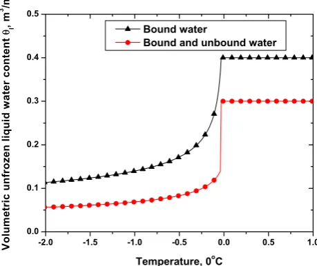
Fig. 1. Typical volumetric content of the unfrozen liquid water in soils as a function of temperature. The curve marked by triangles is associated with soils in which all water is bound in soil pores, and hence the water content gradually decreases with decreasing tem-perature in◦C. To compute this curve we used parametrization (3) in whichT∗=−0.03◦C andb=0.3. The curve marked by circles is
related to soils in which some percentage of water is not bound to the soil particle and changes its phase at the temperatureT∗, while
other part of liquid water is bound in soil pores and freezes gradu-ally as the temperature decreases.
whereφ=φ (T , x)represents the liquid pore water fraction, andT is in◦C, see the curve marked by triangles in Fig. 1.
Note that the constantsT∗andbare the only parameters that
specify dependence of the unfrozen liquid water content on temperature. For example, small values ofbdescribe the liq-uid water content in some fine-grained soils, whereas large values ofb are related to coarse-grained materials in which almost all water freezes at the temperatureT∗. The limiting
case in which all water freezes at the temperatureT∗ is
as-sociated with phase change between water and ice (no soil particles). This limiting case is commonly called the clas-sical Stefan problem and is represented by extremely large values ofbin (3).
In this article, we use the following notation and defini-tions. We abbreviate by lettersi,l ands, ice, liquid water, and the soil particles, respectively. We express thermal con-ductivityλ of the soil and its apparent volumetric heat ca-pacityCapp according to (de Vries, 1963; Sass et al., 1971)
as
λ(T )=λθs
s λ θi(T )
i λ θl(T )
l , Capp(T )=C(T )+L
dθl(T )
dT (4)
Table 1. A typical thickness of soil layers and commonly occurring range of thermal properties in a cryosol soil at the North Slope, Alaska.
Layer Layer thickness Thermal conductivity Porosity, Coefficient in (3)
in the frozen state,λf η b
Moss or organic layer 0.05 [0.1,0.7] [0.1,0.7] [1.0,0.5]
Mineral-organic mixture 0.20 [0.9,1.6] [0.2,0.6] [0.8,0.5]
Mineral soil >1.0 [1.3,2.4] [0.2,0.4] [0.7,0.5]
capacity and thermal conductivity of thek-th constituent at 0◦C, respectively. The quantityθk,k∈{i, l, s}is the volume fraction of each constituent. Exploiting the relationsθs=1−η andθi=η−θl, we introduce notation for the effective volu-metric heat capacitiesCf andCt, and the effective thermal conductivitiesλf andλt of soil for frozen and thawed states, respectively. Therefore formulae (4) and (5) yield
Capp=C+L
dθl
dT, C=Cf(1−φ)+Ctφ, λ=λ 1−φ f λ
φ t, (6) where
λf=λ1s−ηλ η
i, λt=λ
1−η s λ
η l
Cf=Cs(1−η)+Ciη, Ct=Cs(1−η)+Clη.
For most soils, seasonal deformation of the soil skeleton is negligible, and hence temporal variations in the total soil porosity η for each layer are insignificant. Therefore, the thawed and frozen thermal conductivities for the fully satu-rated soil satisfy
λt
λf =hλl
λi
iη
. (7)
It is important to emphasize that evaporation from the ground surface and from within the upper organic layer can cause partial saturation of upper soil horizons (Hinzman et al., 1991; Kane et al., 2001). Therefore, formula (7) need not hold within live vegetation and organic soil layers, and pos-sibly within organically enriched mineral soil (Romanovsky and Osterkamp, 1997).
In this article, we approximate the coefficientsCapp,λ
ac-cording to (6), where the thermal propertiesλf, λt,Cf, Ct and parametersη, T∗, bare constants within each soil
hori-zon. Table 1 lists typical soil horizon geometry, commonly occurring ranges for the porosityη, thermal conductivityλf and the values ofbparameterizing the unfrozen water con-tent.
3 Solution of the heat equation with phase change
3.1 A review of numerical methods
In order to solve the inverse problem one needs to compute a series of direct problems, i.e. to obtain the temperature fields
for various combinations of thermal properties. A number of numerical methods (Javierre et al., 2006) exist to compute temperature that satisfies the heat equation with phase change (2). These methods vary from the simplest ones which yield inaccurate results to sophisticated ones which produce ac-curate temperature distributions. The highly sophisticated methods explicitly track a region where the phase change occurs and produce a grid refinement in its vicinity, and therefore take significantly more computational time to ob-tain temperature dynamics. Implementing such complicated methods is not always necessary, since an extremely accurate solution is not particularly important when the mathematical model describing nature is significantly simplified.
In this subsection, we briefly review several fixed grid techniques (Voller and Swaminathan, 1990) that accurately estimate soil temperature dynamics and easily extend to multi-dimensional versions of the heat Eq. (2). These meth-ods provide the solution for arbitrary temperature-dependent thermal properties of the soil and do not explicitly track the area where the phase change occurs. Recall that in soils the phase change occurs at almost all sub-zero temperatures. A cornerstone of the fixed grid techniques is a numerical ap-proximation of the apparent heat capacity Capp. A variety
of the approximation techniques can be found in (Voller and Swaminathan, 1990; Pham, 1995) and references therein. In general, two classes of them can be identified. The first class is based on temperature/coordinate averaging (Comini et al., 1974; Lemmon, 1979) of the phase change. Here, the appar-ent heat capacity is approximated by
Capp = ∂H
∂x
∂T
∂x −1
, (8)
where
H =
Z T
0
CappdT ,
is the enthalpy. The second class of methods is based on temperature/time averaging (Morgan et al., 1978). In this approach,
Capp =
Hcurrent−Hprevious
Tcurrent−Tprevious
, (9)
where subscripts mark time steps at which the values ofH
they work best in the case of a naturally occurring wide phase change interval. Also, it is important to note that the approx-imation (8) is not accurate for near zero temperature gradi-ents. In the case when the boundary conditions are given by natural variability (several seasonal freezing/thawing cy-cles), near zero gradients at some depths may occur for some time intervals. Hence, the temperature dynamics calculated by using (8) can have large computational errors.
An alternative fixed grid technique can be developed by rewriting the heat equation (2) in a new form:
∂H ∂t =
∂ ∂xλ
∂
∂xT , T =T (H ), (10)
resulting in the enthalpy diffusion method (Mundim and Fortes, 1979). Advantages of discretizing (10) is that the temperature T=T (H )is a smooth function of enthalpy H
and hence one can compute all partial derivatives. However, for soils with a sharp boundary between thawed and com-pletely frozen states, the enthalpyH becomes a multivariate function when temperatureT nearsT∗. Therefore, solution
of (10) results in that the front becomes artificially stretched over at least one or even several finite elements.
In this article, we propose a fixed grid technique that ap-plies the basic finite element method (Zienkiewicz and Tay-lor, 1991) to Eq. (2). Finite element discretization of
L∂θl ∂t =L
dθl
dT ∂T
∂t
in the left hand side of (2) results in
Z x1
x0
ψi(x)ψj(x)L
dθl
dT T (x, t )
dx dTj
dt , (11)
where ψi(x) and ψi(x) are two piecewise linear basis functions at nodes i and j, respectively, Tj(t ) is the value of temperature at the j-th node at time t, and
T (x, t )=P
iψi(x)Ti(t ). We propose to evaluate this type of integrals using the unfrozen liquid water contentθlas the integration variable, i.e.
Z x1
x0
ψ (x)Ldθl
dT T (x, t )
dx=L Z θ1
θ0
ψ T (θl, t )
dθl, (12) whereψ=ψiψj, andθ0=θl(T (x0, t ))andθ1=θl(T (x1, t )).
This substitution allows precise computation of the latent heat effect for arbitrary grid cells, since it is parameterized by the limits of integrationθ0, θ1, instead of being
calcu-lated using the rapidly varying function dθl
dT(T ) on the el-ement[x0, x1] by a quadrature rule. As a consequence of
the proposed substitution, evaluation of the integral in (11) may not to yield the right result unless the functionT (θl) must be monotonically increasing for allθl<η, andT (x, t ) be monotonous on [x0, x1]at time t. Figure 1 shows two
instances of the unfrozen water content curves frequently oc-curring in nature. The curve marked by circles is associated with soils in which free water freezes prior to freezing of the
bound liquid water in soil pores. The free water is associ-ated with a vertical line atT=T∗whereas the bound water is
represented by a smooth curve atT <T∗. The curve marked
by triangles reflects soil in which all water is bounded in soil pores and can be parameterized by (3) used in our modeling. 3.2 Finite element formulation
Let us consider a triangulation of the interval[0, l]by a set of nodes{xi}ni=1. With each nodexi, we associate a contin-uous functionψi(x)such thatψi(xj)=δij. We will refer to {ψi}ni=1 as the basis functions on the interval[0, l]. Hence,
the temperatureT (x, t )on[0, l]is approximated by a linear combination:T (x, t )=Pn
i=1Ti(t )ψi(x), whereTi=Ti(t )is the temperature at the nodexi at the timet. Substituting this linear combination into (2), multiplying it byψj and then integrating over the interval[0, l], we obtain a system of dif-ferential equations (Zienkiewicz and Taylor, 1991):
M(T)d
dtT(t )= −K(T)T(t ), (13)
where T≡T(t )=[T1(t ) T2(t ) . . . Tn(t )]t is the vector of tem-peratures at nodes{xi}ni=1at timet. Here, then×nmatrices M(T)={mij}nij=1and K(T)={kij}
n
ij=1are mass and stiffness
matrices, respectively. Entry-wise they are defined as
mij=
Z l
0
C(T , x)ψiψjdx+L
Z l
0 dθl
dTψiψjdx (14)
kij=
Z l
0
λ(T , x)dψi dx
dψj
dx dx. (15)
The fully implicit scheme is utilized to discretize (13) with respect to time. Denoting bydtk the time increment at the
k-th moment of timetk, one has
Mk+dtkKk
Tk=MkTk−1, k >1 (16)
where Tk=T(tk), Kk=K(Tk), Mk=M(Tk). We impose boundary conditions atx=0 and some depth x=l by spec-ifyingT1(tk)=Tu(tk)andTn(tk)=Tl(tk).
Given Tk−1, we find the solution Tk of (16) by Picard it-eration (Kolmogorov and Fomin, 1975). The itit-eration pro-cess starts from the initial guess Tk0 = Tk−1that is used to compute temperature Tk1at the first iteration. At iterations, we compute Tk
s and terminate iterations atse when a cer-tain convergence condition is met. The value of Tks is used to evaluate the matrices Mks=M(Tks), and Kks=K(Tks). In turn, these are utilized to compute thes+1 iteration Tks+1by equating
[Mks +dtkKks]Tks+1−MksTk−1=0. (17) At each iteration the convergence condition maxk|Tks+1(tk)−Tks(tk)|≤ is checked. If it hold, the iterations are terminated at se=s+1. If the number of iterations exceeds a certain predefined number, the time incrementdtkis halved and the iterations start again. Please, note that the convergence is guaranteed if the time increment
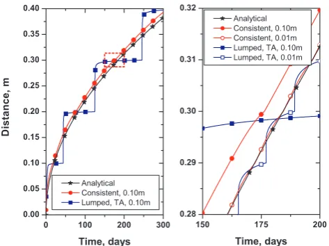
Fig. 2. Comparison of analytical (stars) and numerical solutions. Initially, the soil has−5◦C temperature, and at the timet=0, the temperature at its upper boundary is changed to 1◦C. At the lower boundary located at 5 m depth, zero flux boundary condition is spec-ified. On the left plot, we show a location of the 0◦C isotherm calcu-lated for a uniform spatial discretizations with 0.1 m grid element. The numerical solutions are computed by the proposed method (cir-cles) and by the scheme using the lumped approach with temporal enthalpy averaging (squares). In the right plot, we show an enlarged area within the dotted rectangle and a location of the 0◦C isotherm calculated for a uniform spatial discretizations with 0.1 m (filled) and 0.01 m (hollow) grid elements.
3.3 Computation of the mass matrix
One of the obstacles to obtain a finite dimensional approxi-mation that accurately captures the temperature dynamics is related to evaluation of the mass matrix M. Since the basis functionψidoes not vanish only on the interval[xi−1, xi+1],
the matrix M is tri-diagonal. Therefore, to compute itsi-th row we evaluate
Z l
0 dθl
dTψj(x)ψi(x)dx j =i−1, i, i+1, (18)
wherejstands for the column index. For the sake of brevity, we consider the first integral (j=i−1) in (18). This restricts us only to the grid element[xi−1, xi], yielding
Z l
0 dθl
dTψi−1(x)ψi(x)dx= Z xi
x−1 dθl
dTψi−1(x)ψi(x)dx. (19)
We recall that in the standard finite element method, the tem-perature on the interval[xi−1xi]is approximated by
T (x, t )=ψi−1(x)Ti−1(t )+ψi(x)Ti(t ), (20) for anyx ∈ [xi−1, xi]and fixed moment timet. Here,ψi and
ψi−1are piece-wise linear functions satisfyingψi−1=1−ψi on[xi−1, xi]. For allx ∈ [xi−1, xi], we can compute the tem-peratureT from (20) and values ofTi,Ti−1. Note that in the
case of1Ti=0, we can compute (19) directly sincedθl/dT is constant over [xi−1xi]. However, if 1Ti=Ti−Ti−16=0,
then we can consider an inverse function, that is,x is taken as a function ofT to obtain
Z xi
xi−1 dθl
dTψi−1ψidx=
xi−xi−1 (1Ti)3
Z xi
xi−1 dθl
dT(Ti−T )(T−Ti−1)dT
Therefore
Z l
0 dθl
dTψi−1ψidx=
xi −xi−1 (1Ti)3
Z θi
θi−1
(T −Ti)(Ti−1−T )dθ,
(21) whereθi−1=θl(T (xi−1, t ))andθi=θl(T (xi, t )). Note that in (21) the temperatureT is a function of the liquid water con-tentθl, i.e.T=θl−1(θl). Therefore, returning back to (18), we have that each of the integrals in (18) is a linear combination of the typeβ2A2+β1A1+β0A0, where
Ak=
Z θi
θi−1
[θl−1(z)]kdz, k=0,1,2.
The constants{βk}are easily computable ifθl(T )is given by (3).
3.4 Evaluation of the proposed method
To test the proposed method, we compare temperature dy-namics computed by the proposed method with an analytical solution of the heat Eq. (2) in whichb→∞. This analytical solution is called Neumann solution (Gupta, 2003) and is typ-ically used to verify numerical schemes. In the proposed nu-merical scheme the mass matrix M is tri-diagonal, and hence this scheme is called consistent. Other commonly utilized numerical schemes are called mass lumped (Zienkiewicz and Taylor, 1991) since they employ the diagonal mass matrix:
M=diag(Capp,1
Z 1
0
ψ1dx, . . . , Capp,n
Z 1
0
ψndx). (22) Here,Capp,iis the value of the apparent heat capacityCappat
thei-th node computed either by spatial (8) or temporal (9) averaging of latent heat effects.
In Fig. 2, we compare temperature dynamics computed by the proposed consistent and a typical mass lumped scheme. We plot a location of the 0◦C isotherm for several spatial dis-cretizations, i.e. the distance1xi between two neighboring nodes xi andxi−1 is 0.1 or 0.01 m. In this figure we see
that the location of the 0◦C isotherm calculated by
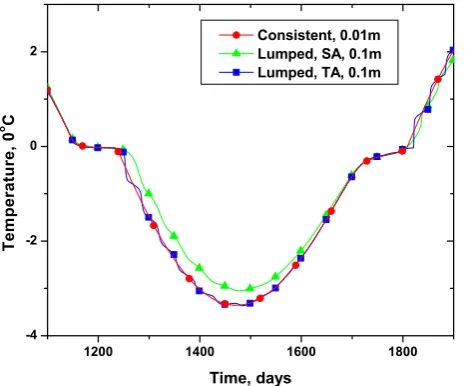
Fig. 3. Computed soil temperature dynamics at 0.3 m depth. Uni-form 0.01 and 0.1 m meshes are used to compute temperatures by the consistent (circles) and mass lumped approaches, respectively. The spatial (SA) and temporal (TA) enthalpy averaging in lumped schemes are marked my triangles and squares, respectively. Ini-tially the temperature is zero, the upper boundary condition is given by Dirichlet type boundary condition with a slowly varying sinusoid having the amplitude of 3◦C and the period of there years; zero heat flux is specified at 2 m depth.
gives a better solution and smoother rate of advancing of the 0◦C isotherm, see Fig. 2, left.
In Fig. 3, we compare temperature dynamics computed by two mass lumped approaches exploiting spatial (8) and tem-poral (9) enthalpy averaging. A warm bias in the tempera-ture computed by the spatial averaging of the enthalpy is due to computational errors occurring when the temperature gra-dient is approximately zero at some depth. Our experience shows that this difference appears regardless of decreasing the tolerancebetween iterations in (17). We note that in all above numerical experiments a finite element computer code is the same except for a part associated with computation of mass matrix, i.e. consistent (18) or mass lumped (22). These numerical experiments show that the straight-forward mass lumped schemes are typically inferior to consistent ones.
Since our method (14) is based on the consistent approach (the mass matrix M is the tri-diagonal one), the numerical solution oscillates if the time stepsdtk are too small (Pin-der and Gray, 1977). For a fixed time stepdtk, the oscilla-tions disappear if the spatial discretization becomes fine, i.e. the inequalitymij+dtkkij<0 holds wheni6=j(Ciarlet, 2002; Dalhuijsen and Segal, 1986). It is shown that these oscilla-tions occur due to violation of the discrete maximum princi-ple (Rank et al., 1983). Therefore, to avoid the oscillations in the numerical solution (Dalhuijsen and Segal, 1986), we propose either to use sufficiently large time steps (for which
Fig. 4. Temperature dynamics at 1 m depth computed by the pro-posed consistent (circles) and the mass lumped schemes (stars). The mass lumped scheme is based on (23). In order to emphasis numer-ical oscillations occurring in the case of small time steps in the con-sistent approach, we use a uniform grid with 0.1 m grid elements. The oscillations are due to violation of the discrete maximum prin-ciple in the consistent scheme during active phase change processes. The initial and boundary conditions are the same as stated in caption of Fig. 3.
the formula can be found in the above cited references) or to exploit the following regularization. We construct a lumped versionM˜={ ˜mij}of the mass matrix M given by
˜
mii=
X
j
mij (23)
and substituteM for M in (16). Comparison of temperature˜ dynamics computed employing the proposed consistent M defined by (16) and its mass lumped modificationM defined˜ by (23) is shown in Fig. 4. The numerical oscillations near 0◦C disappear in the temperature dynamics computed by the proposed mass lumped approach (see Fig. 4). In Fig. 5, we compare the proposed mass lumped approach (stars), and the one based on temporal enthalpy averaging (squares) by (8). This figure shows that the numerical scheme using tempo-ral averaging of the enthalpy produces larger oscillation than our solution. This comparison reveals that the proposed mass lumped approach (23) reduces some numerical oscillations and follows the “exact” solution (computed by the consis-tent approach with a fine spatial discretization) more closely than the solution computed by the lumped approach exploit-ing (8).
Fig. 5. Temperature dynamics at 1 m depth computed by the consis-tent approach (circles), the proposed mass lumped approach (stars) and the mass lumped approach with temporal enthalpy averaging (squares). The temperatures computed mass lumped approach are found on uniform grid with 0.1 m grid elements, whereas in the con-sistent approach, the length of grid elements is 0.01 m. The initial and boundary conditions are the same as stated in caption of Fig. 3.
coarse spatial discretization, consistent schemes can violate the discrete maximum principle, and hence the mass lumped schemes are more attractive. In this article, we construct a fine spatial discretization and use the proposed consistent ap-proach, while restricting the time steptk from below.
4 Variational approach to find the soil properties
In this section, we provide definitions and describe main components of the indirect method used to find the soil prop-erties by minimizing the cost function outlined in (1).
We define the controlCas a set consisting of thermal con-ductivitiesλ(i)t , λ(i)f , heat capacitiesCt(i), Cf(i)and parameters
η(i), T∗(i), b(i)describing the unfrozen water content for each
soil horizoni=1, . . . , n, or
C= {C(i)f , C(i)t , λ(i)t , λ(i)f , η(i), T∗(i), b(i)}n
i=1, (24)
wherenis the total number of horizons. We say that a solu-tion of the direct problem for the controlCisT (x, t;C)and is defined by the set
T (x, t;C)= {T (xi, t ):i=1, . . . , m;t ∈ [0, τ]}, (25) where{xi}mi=1is a set ofmfixed distinct points on[0,l]. In
(25), theT (xi, t )are point-wise values of temperature dis-tributions satisfying (2) in which thermal properties of each horizon are given according toC.
The counterpart ofT (x, t;C)is the dataTD(x, t )defined by a set of measured temperature at the same depths{xi}mi=1
and the same time interval[0, τ]. Since the dataTD(x, t )and its model counterpartT (x, t;C)are given on the same set of depths and time interval, we can easily compute a discrep-ancy between them, usually measured by the cost function J (C)= 1
m(ts−te) m
X
i=1
1
σi2
Z te
ts
(TD(xi, t )−T (xi, t;C))2dt. (26)
Here,ts, te ∈ [0, τ]andσi stands for an uncertainty in mea-surements by thei-th sensor. In our measurements all tem-perature sensors assume the same precision, so all of{σi}are equal. Given a way to measure this discrepancy as in (26) we can finally formulate an inverse problem.
For the given dataTD(x, t ), we say that the control C∗
is a solution to an inverse problem if discrepancy between the data and its model counterpart evaluated atC∗ is
mini-mal (Alifanov, 1995; Alifanov et al., 1996; Tikhonov et al., 1996). That is,
J (C∗)=min
C J (C).
To illustrate steps which are necessary to solve this inverse problem and find an optimalC∗ we provide the following
example. To formulate the inverse problem one has to have the measured temperaturesTD(x, t ). For the sake of this ex-ample, we replace the dataTD(x, t )by a synthetic tempera-tureTS(x, t ) =T (x, t;C0)(a numerical solution of the heat Eq. (2) for the known combinationC0of the thermal proper-ties):
C0=
C(f1)=1.6×10⁶, C(1) t =2.1×10⁶, λ
(1) f=0.55, λ
(1)
t =0.14, η(1)=0.30, b(1)=0.9, T (1)
∗ =−0.03 C(f2)=1.7×10⁶, C
(2)
t =2.3×10⁶, λf(2)=0.90, λ (2)
t =0.66, η(2)=0.30, b(2)=0.6, T∗(2)=−0.03 C(f3)=1.8×10⁶, C
(3) t =2.6×10⁶, λ
(3) f=1.90, λ
(3)
t =1.25, η(3)=0.25, b(3)=0.8, T (3)
∗ =−0.03
.
The initial and boundary conditions in all calculations are fixed and given by in-situ temperature measurements in 2001 and 2002 at the Happy Valley site located in the Alaskan Arctic. We compute the temperature dynamics for a soil slab with dimensions[0.02,1.06]between 21 July 2001 and 6 May 2002, and evaluate the cost function at{xi}i={0.10, 0.17, 0.25, 0.32, 0.40, 0.48, 0.55, 0.70, 0.86 m. Uniformly distributed noise on[−0.04,0.04]was added toTS(x, t ), to simulate noisy temperature data recorded by sensors (preci-sion of the sensor is 0.04◦C). The boundaries between the horizons lie at 0.10 and 0.20 m depth.
We find a control C0 that minimizes the cost functionJ
defined by (26) in whichTD(x, t )=TS(x, t ). For the sake of simplicity, we assume that all variables inC0 are known except for the pairλ(f2),η(3). Therefore, the problem of find-ing this pair can be solved by minimizfind-ing the cost function
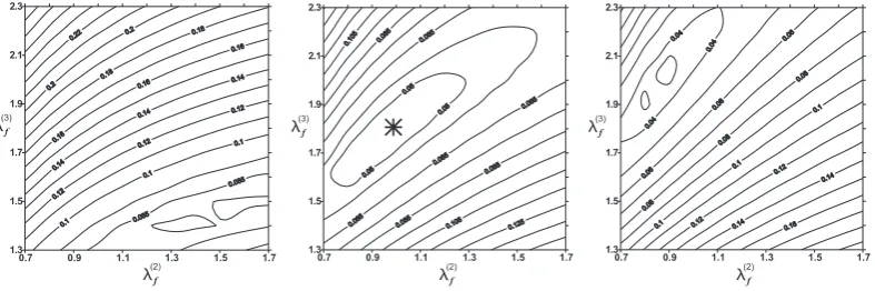
J on(λ(f2),η(3))plane as follows. We compute temperature dynamics for various combinations ofλ(f2),η(3)and plot iso-lines ofJ, see Fig. 6. The point on(λ(f2),η(3))plane where the cost function is minimal gives the sought values ofλ(f2)
In the above example, the control had only two unknown variablesλ(f2), η(3)and we minimized the corresponding cost function. Usually, a majority of variables in the controlCis unknown, and hence multivariate minimization is required. Since computation of the cost function for all possible real-izations of the control on the discrete grid is extremely time-consuming, various iterative techniques are used (Fletcher, 2000).
We note that if the cost function has several minima due to non-linearities of the heat Eq. (2) and if the initial ap-proximationC0is arbitrary then the iterative algorithm can converge to an improper minimum. Nevertheless, with the initial approximationC0within the basin of attraction of the global minimum, the iterative optimization method should converge to the proper minimum even if the model is nonlin-ear (Thacker, 1989). Consequently, proper determination of an initial approximationC0is important.
After selection of the initial approximationC0, the next step is to minimize the cost functionJ (C)with respect to all parameters inC. There is a great variety of iterative methods that minimizeJ (C). The majority of them rely on compu-tation of the gradient∇J (C)of the cost function. The com-putation of∇J (C)is a complicated problem and is out of the scope of this article. An interested reader is referred to (Alifanov et al., 1996; Permyakov, 2004) and to references therein. Since in this article we are primarily concerned with evaluation of the initial approximation to the thermal prop-erties, we use the following universal algorithm to minimize the cost function.
We look for the minimum of the cost function by the simplex search method described in (Lagarias et al., 1998), which is a direct search method (Bazaraa et al., 1993). In a two and three dimensional spaces, the simplex is a trian-gle or a pyramid, respectively. At each iteration the value of the function computed at the point, being in or near the cur-rent simplex, is compared with the function’s values at the vertices of the simplex and, usually, one of the vertices is re-placed by the new point, giving a new simplex. The iteration processes is continued until the simplex sizes are less than an a priori specified tolerance. At the final iteration, we obtain the setCof parameters that determine the thermal properties, porosity and coefficients specifying the unfrozen water con-tent for each soil horizon. However, we note that this algo-rithm typically converges to the minimum slower than other algorithms that require calculations of the gradient (Dennis and Schnabel, 1987).
5 Selection of an initial approximation
Selection of a proper initial approximationC0 is an impor-tant problem, since the proper choice ofC0ensures that the minimization procedure converges to a global minimum. In this section we describe how to select a proper initial approx-imation by considering several simpler subproblems.
Fig. 6. Isolines of the cost functionJ (C)computed using the
syn-thetic temperature dataTS. The minimum of the cost function is marked by the start and is located atλ(f2)=0.9 andη(3)=0.25, which
is coincide with the values ofλ(f2),η(3)used to computeTS.
5.1 General methodology
We begin by noting that in the natural environment, the ther-mal properties and the water content are confined within a certain range depending on soil texture and mineralogy. Therefore, the coefficients in (2) and hence their initial ap-proximations lie within certain limits. To ensure better deter-mination of the initial approximationC0, we employ an algo-rithm similar to coordinate-wise searching method (Bazaraa et al., 1993). In this method, one looks for a minimum along one coordinate, keeping other coordinates fixed, and then looks for the minimum along another coordinate keeping oth-ers fixed and so on.
We propose to look for a minimum with respect to some subset of parameters inC, followed by a search along other parameters inCand so on. In details, our approach is formu-lated in five steps:
1. Select several time intervals{1k}in the period of ob-servations[0, τ]
2. Associate a certain subsetCjof parametersCwith each
1j. The subsetCj is such that the temperature dynam-ics over the period1j is primarily determined byCj and depend much less on changes in any other parame-ters inC.
3. Select a certain pair {1j,Cj}, and look for a location of the minimum of the cost functionJ (C)keeping all parameters inCexcept forCjfixed.
4. Update values ofCj in the controlCby the results ob-tained at Step 3.
Fig. 7. Temperature dynamics at 0.25 m depth at Happy Valley site during the summer of 2001 year. The graph shows that uncertainty in temperature measurements is±0.02◦C. Within this uncertainty, the shadowed region represents a temperature range where the soil starts to freeze. Therefore, the temperature,T∗, of freezing point
depression lies within the shadowed regions, i.e. in [−0.04◦C/0◦C].
We continue this iterative processes until the difference be-tween the previous and current values of parameters inCis below a critical tolerance.
The selected periods1k do not have to coincide with tra-ditional subdivision of a year. The choice of1k is naturally dictated by seasons in the hydrological year, which starts at the end of summer and consists several seasons. If the period of observations is one year, typical intervals1kare “winter”, “summer and fall”, “fall” and “extended summer and fall”, see Table 2. We note that the intervals1k can overlap each other, and quantitiests andte determining lower and upper limits of integration in (26) are equal to the beginning and end of the time interval1k. For different geographical re-gions, the timing for the “winter”, “summer and fall” and “fall” can be different. Typical timing of periods{1k}for the North Slope of Alaska is shown in Table 2, and are now discussed.
5.2 Subproblems
11: The “winter” period corresponds to the time when the
rate of change of the unfrozen liquid water contentθlis neg-ligibly small; the heat Eq. (2) models the transient heat con-duction with thermal propertiesλ=λf,C=Cf, and dθdTl'0. During the “winter”, temperature dynamics depend only on the thermal diffusivityCf/λf of the frozen soil, and hence the simultaneous determination of both parametersCf and
λf is an ill-conditioned problem. Assuming that the heat capacity{Cf(i)}is known (depending on the soil texture and moisture content we can approximate it using published
data), we evaluate the thermal conductivity {λ(i)f } and use these values during minimization at other intervals.
12: During the “summer and fall” time interval, active
phase change of soil moisture occurs. Hence, at this time, see Table 2, a contribution of the heat capacity C into the apparent heat capacity Capp is negligibly small comparing
to the contribution of the latent heat termLdθl/dT. There-fore, the rate of freezing/thawing primarily depends on the soil porosityηand the thermal conductivityλ(Tikhonov and Samarskii, 1963). Thus we approximate{Ct(i)}using pub-lished data by analyzing the soil texture and moisture con-tent. Note that temperature-dependent latent heat effects due to the existence of unfrozen waterθlat this period have a sec-ond order of magnitude effect (see discussion below). There-fore, if no prior information about the coefficientsb, T∗
pa-rameterizing the unfrozen water content is available then they can be prescribed by taking into account the soil texture and analyzing measured temperature dynamics at the beginning of freeze-up (see Fig. 7). We seek better estimates ofb, T∗at
the next steps, namely during the “fall” period.
Since, during the “summer and fall” interval, the tempera-ture dynamics primarily depends on the porosityηand ther-mal conductivityλ, we have to find only{λ(j )t , η(j )}, since {λ(j )f }are already found at the previous step, i.e. the “winter” interval. Taking into account the relationship (7) between the thermal conductivities for completely frozen and thawed soil, we approximate
λ(j )t =λ(j )f hλl λi
iη(j )
, j =2, . . . , n. (27)
We remind that the water contentθlin the upper soil horizon changes during the year due to moisture evaporation and pre-cipitation and is not always equal toη(1). Hence formula (27) does not hold forj=1. Hence, during the “summer and fall” period our goal is to estimate{η(i)}n
i=1andλ
(1)
t , and then de-termine thermal conductivityλ(j )t for the rest of soil layers
j=2, . . ., nusing (27).
13: Recall that while evaluating the thermal properties {λ(i)t , λ(i)f }and the soil porosity{η(i)}, we assumed that the coefficients{b(i), T∗(i)}are known. However they also have
to be determined. We remind that the coefficients{b(i), T∗(i)}
cannot be computed prior to calculation of{λ(i)t , λ(i)f } and {η(i)}, since{b(i), T∗(i)}are related to the second order effects
in temperature dynamics during “summer and fall” and “win-ter” intervals. Once an initial approximation to {λ(i)t , λ(i)f } and{η(i)}is established, we consider the “fall” period (see Table 2) during which the temperature dynamics strongly de-pends on{b(i), T∗(i)}and allows us to capture second order
ef-fects in temperature dynamics (Osterkamp and Romanovsky, 1997).
14: In the previous three periods, we obtained
Table 2. Typical choice of parameters in the controlCfor “cold” permafrost regions.
Periods Cj Typical1k Characteristic Step
“Winter” {λ(i)f } December–April Completely frozen ground,T <−5◦C 1
“Summer and Fall” {η(i)},λ(t1) May–November Developing/-ed active layer and its freezing 2
“Fall” {b(i),T∗(i)} September–December Active layer freezing,T >−5◦C 3
“Extended Summer and Fall” {η(i),T∗(i)} May–January Developing/-ed active layer and its freezing 4
However, we can improve the approximation by consider-ing the “extended summer and fall” period, see Table 2. This period is associated with a time interval when the soil first thaws and then later becomes completely frozen. Since previously, we minimized the cost function depending sep-arately on the porosity {η(i)} (“summer and fall”) and on {T∗(i)}(“fall”), we minimize the cost function depending
si-multaneously on{η(i)}and{T∗(i)}during “extended summer
and fall”, while other parameters are fixed.
We list in Table 2 all steps and time periods1k which are necessary to find the initial approximation. One of the sequences of minimization steps is
“winter” →“summer and fall”→ “fall” →“extended summer and fall”
From our experience with this algorithm, we conclude that in some circumstances it is necessary to repeat minimization over some time periods several times, e.g.
“winter” →“summer and fall”→
“fall” →“extended summer and fall”→ “fall” →“extended summer and fall”
until the consecutive iterations modify the thermal properties insignificantly.
6 Application. Happy Valley site
6.1 Short site description
The temperature measurements were taken in the tussock tundra site located at the Happy Valley (69◦80N ,148◦500W) in the northern foothills of the Brooks Range in Alaska from 22 July 2001 until 22 February 2005. We used data from 22 July 2001 until 15 May 2002 to estimate soil properties, and from 15 May 2002 until 22 February 2005 to validate the estimated properties. The site was instrumented by eleven thermistors arranged vertically at depths of 0.02, 0.10, 0.17, 0.25, 0.32, 0.40, 0.48, 0.55, 0.70, 0.86 and 1.06 m. The tem-perature sensors were embedded into a plastic pipe (the MRC probe), that was inserted into a small diameter hole drilled into the ground. The empty space between the MRC and the ground was filled with a slurry of similar material to diminish an impact of the probe to the thermal regime of soil. Our frost heave measurements show that the vertical displacement of the ground versus the MRC probe is negligibly small at this
particular installation site. Prior to the installation, all sen-sors were referenced to 0◦C in an ice slush bath and have
the precision of 0.04◦C. An automatic reading of
tempera-ture were taken every five minutes, then averaged hourly and stored in a data logger memory.
During the installation, soil horizons were described and their thicknesses were measured. The soil has three distinct horizons: organic cover, organically enriched mineral soil, and mineral soil. The boundaries between the horizons lie at 0.10 and 0.20 m depth.
In the all following numerical simulations we consider a slab of ground representing the Happy Valley soil between 0.02 and 1.06 m depth. For the computational purposes, the upper and lower boundary conditions are given by the ob-served temperatures at depth of 0.02 and 1.06 m. Also in all computations, the temperatures are compared with the set of measured temperatures at the depths{xi}={0.10, 0.17, 0.25, 0.32, 0.40, 0.48, 0.55, 0.70, 0.86}m.
6.2 Selection of an initial approximation
The “winter” period is associated to the ground temperature below−5◦C, occurring on 15 January 2002 through 15 May
2002 at the Happy Valley site. The heat capacityCf for each layer is evaluated based on the soil type, texture and is taken from (Hinzman et al., 1991; Romanovsky and Osterkamp, 1995; Osterkamp and Romanovsky, 1996).
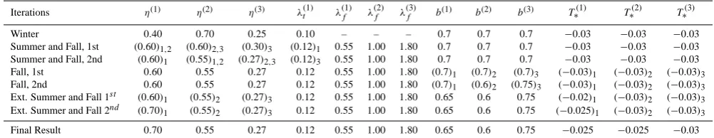
We estimateλf for each layer by looking for a minimum of the cost function J in the 3-D space {λ(f1), λf(2), λ(f3)}. The minimization problem in this space can be simplified by looking for a minimum in the following series of 2-D prob-lems. For example, for several physically acceptable values of the thermal conductivityλ(f1), we compute temperature dy-namics for various values ofλ(f2),λ(f3)and plot isolines of the cost functionJ. In the series of plots in Fig. 8, we notice that a location of the minimum on the(λ(f2), λ(f3))plane shifts asλ(f1) changes. The minimum of the cost function at each cross section is almost the same, and the problem of selecting the right combination of parameters arises. Here, knowledge of the soil structure becomes relevant. It is known that the soil type of third layer is silt highly enriched with ice, so from Table 1 1.6<λ(f3)<2.0. Therefore, we selectλ(f1)=0.55,
Fig. 8. The isolines of the cost functionJ on the plane(λ(f2), λf(3))for different values of the thermal conductivityλ(f1)keeping constant
at each plot. The values ofλ(f1)from the left to the right are 0.35, 0.55 are 0.70, respectively. The star in the central plot marks a selected combination of the thermal conductivities.
steps (see Table 3, columns 6,7 and 8). More precise results could be obtained if a sensor measuring the thermal conduc-tivity was placed in at least one of the horizons, see discus-sion in Sect. 7.
The “summer and fall” period is selected to capture the maximal depth of active layer occurring between 28 Au-gust 2001 and 6 December 2001. We take values of the heat capacityCt from (Hinzman et al., 1991; Romanovsky and Osterkamp, 1995; Osterkamp and Romanovsky, 1996). Comparing measured temperatures to the ones computed for λ(t1), {η(i)}3
i=1 varying within a range of their natural
variability, we found thatλ(t1)∈[0.09,0.15],η(1)∈[0.3,0.9],
η(2)∈[0.3,0.9]andη(3)∈[0.15,0.45]. Once the variability of these parameters is found, we search for a minimum of the cost function in the 4-D space{λ(t1), η(1), η(2), η(3)}, where each parameter varies within the found boundaries. We note that during minimization ofJ in this 4-D space, other vari-ables inCare fixed and their values are listed in 1st “Summer and Fall” row in Table 3. For example, values of the thermal conductivityλ(f1)=0.55,λf(2)=1.0 andλ(f3)=1.8 are obtained at the previous step after minimization over the “winter” in-terval. Also, an approximation to the coefficientsb(i)=0.7,
T∗(i)=−0.03,i=1,2,3 in (3) is obtained by analyzing soil
texture and type, and dynamics of the measured temperatures near 0◦C, see Fig. 7. We emphasis that the approximation to
the parametersbandT∗ is tentative and is going to be
im-proved at the consequent steps.
We note that it is not necessary to find a minimum in the four dimensional space accurately but rather only to estimate its location as significant uncertainties in other parameters still exist. Therefore, we look for the minimum by evaluating the cost function on(λ(t1), η(1)), (η(1), η(2))and(η(2), η(3))
planes as follows.
First, we setη(1)=0.6,η(2)=0.6,η(3)=0.3 andλ(t1)=0.12, which correspond to the middle of their variability ranges. Then, we evaluate the cost function J on the (λ(t1), η(1))
plane, by varying λ(t1), η(1) in the control, while all other variables inCare fixed. In the left plot in Fig. 9, we plot isolines ofJ on all three planes(λ(t1), η(1)),(η(1), η(2)), and
(η(2), η(3)).
At the(λ(t1), η(1))plane, the cost function attains its min-imal value on a boundary of this plane, see Fig. 9, upper left, and is minimal in the center of the planes(η(1), η(2)),
(η(2), η(3)). The last two planes allows us to find that
η(1)=0.6,η(2)=0.55 andη(3)=0.27, whereas contours at the first plane show that the value ofλ(t1)lies between 0.11 and 0.13, see Fig. 9, left column. We suppose thatλ(t1) is 0.12 and proceed further. After updating the control with the com-puted values, we evaluate the cost function on the same set of planes one more time; parameters in the control before minimization are shown in Table 3 the “Summer and Fall” 2nd row. After computing the cost function, we draw its iso-lines and show them in Fig. 9, right. Note that at this step the cost function attains its minima located in the center of the computational grid. We update the control withη(1)=0.6,
η(2)=0.55,η(3)=0.27,λ(t1)=0.12. Note that the location of the minimum did not change significantly. Our experience shows that changes of soil properties by 5%–10% or less are insignificant, since the corresponding difference in soil tem-peratures is comparable with uncertainties of measurements. Therefore, we do not have to do additional iterations on the same set of planes, and we proceed to the next step and re-duce uncertainties in coefficientsT∗andb.
Table 3. Values of parameters in the control at the beginning of each minimization step. The listed steps are typical to recover the initial approximation to the soil properties. The parameters which values are in the parenthesis with the same subindex define minimization plane. For example, in the third rowλ(t1) andη(1) are in the parenthesis and have the same subindex equal to 1. Therefore, this pair define a
minimization plane(λ(t1), η(1)). On this plane we minimize the cost function depending onλ(t1)andη(1), while value of other parameters are fixed and given in other sections of the current row.
Iterations η(1) η(2) η(3) λ(t1) λ(f1) λ(f2) λf(3) b(1) b(2) b(3) T∗(1) T∗(2) T∗(3)
Winter 0.40 0.70 0.25 0.10 – – – 0.7 0.7 0.7 −0.03 −0.03 −0.03 Summer and Fall, 1st (0.60)1,2 (0.60)2,3 (0.30)3 (0.12)1 0.55 1.00 1.80 0.7 0.7 0.7 −0.03 −0.03 −0.03 Summer and Fall, 2nd (0.60)1 (0.55)1,2 (0.27)2,3 (0.12)3 0.55 1.00 1.80 0.7 0.7 0.7 −0.03 −0.03 −0.03 Fall, 1st 0.60 0.55 0.27 0.12 0.55 1.00 1.80 (0.7)1 (0.7)2 (0.7)3 (−0.03)1 (−0.03)2 (−0.03)3 Fall, 2nd 0.60 0.55 0.27 0.12 0.55 1.00 1.80 (0.7)1 (0.6)2 (0.75)3 (−0.03)1 (−0.03)2 (−0.03)3 Ext. Summer and Fall 1st (0.60)
1 (0.55)2 (0.27)3 0.12 0.55 1.00 1.80 0.65 0.6 0.75 (−0.02)1 (−0.03)2 (−0.03)3 Ext. Summer and Fall 2nd (0.70)
1 (0.55)2 (0.27)3 0.12 0.55 1.00 1.80 0.65 0.6 0.75 (−0.025)1 (−0.03)2 (−0.03)3 Final Result 0.70 0.55 0.27 0.12 0.55 1.00 1.80 0.65 0.6 0.75 −0.025 −0.025 −0.03
6.3 Global minimization and sensitivity analysis
While evaluating an initial approximation, we sought minima of the cost functionsJ (C)measuring discrepancy over peri-ods{1k}. In this subsection, we perform global minimiza-tion of the cost funcminimiza-tion with respect to all parameters inC over the entire period of measurements 22 July 2001 until 15 May 2002 used for calibration. Also, we analyze sensitivity of an initial approximation derived from minimizing the cost function globally with respect to all parameters.
In global minimization problems, a starting point from which iterations begin is given by the initial approximation evaluated in the previous subsection, see Table 3, the last row. As a result of global minimization problem, we obtain the parameters (thermal properties, porosity and coefficients specifying the unfrozen water content for each soil horizon) which can depend on valuests andtedetermining the period over which discrepancy between observed and modeled tem-peratures is measured. In global minimization problems, the constantteis associated with an end of “winter” interval dur-ing which the soil is completely frozen. But since, the soil is frozen for several months for a cold permafrost region, the cost function does not significantly depends onteiftevaries within two week limits. However, the value ofts is asso-ciated with beginning of “summer and fall” interval during which the ground is thawed. Since, the ground is thawing during a relatively short period of time for cold permafrost regions, we consider several values ofts and minimize the cost function with respect to all parameters.
Results of minimization are listed in Table 4. It shows that the results of global minimization do not significantly depend on constantsts, if the interval[ts, te]represents thawed and frozen states of the soil. Using averaged values of the ther-mal properties, we compute the temperature dynamics for the entire period of observations. Comparison of the calculated and measured temperatures at different depths and at time in-tervals used for calibration are shown in Figs. 10, 11 and 12. During the winter, the calculated temperature closely follows
the observed temperature within the uncertainty of thermistor measurements. During the summer, the difference between the measured and calculated temperatures is larger but does not exceed 0.3◦C for sensors in the mineral soil. This larger discrepancy between the measured and computed tempera-tures can be partially explained by over-simplifying physics and neglecting water dynamics in the upper organic horizons. Finally, in order to show that the found initial approxima-tion (the last row in Table 3) lies close to the true values of soil properties, we use it to compute the soil temperature dy-namics through 22 February 2005. Note that the time interval from 22 May 2002 until 22 February 2005 was not used to find the soil properties. In Fig. 13, we plot the measured and calculated temperature dynamics at 0.55 m depths. The plots with solid symbols mark temperature dynamics com-puted for the found initial approximation, and for the best guess values (in the middle of the variability range, shown in Table 1). We note that the guessed values are used to provide benchmark temperature dynamics against which we show ef-fectiveness of our approach. The benchmark temperature is much warmer during summer, and the freeze-up occurs sev-eral days later than in the measured temperature. The bench-mark temperature dynamics during winter closely follows the measured temperature dynamics, since the middle of the variability range, for which the benchmark temperature was computed, almost matches the found initial approximation. The difference between the measured temperature dynamics and the one calculated for the found initial approximation is typically less than 0.25◦C.
7 Discussion and limitation of the proposed method
Fig. 9. Selection of the thermal conductivityλ(t1)and the soil porosityη(1),η(2),η(3)by minimizing the cost function associated with the “summer and fall” interval. The left and right column are associated with the first and the second iterations, respectively. The stars mark selected values of parameters after completing the iteration. Note that at the second iteration stars and locations of all minima are coincide.
select the initial approximation to the soil properties. For ex-ample, if the gradient type algorithm is started outside the basin of attraction of the proper minimum, then due to exis-tence of multiple local minima it can converge to physically non-realistic combination of parameters inC. Stochastic and heuristic algorithms can possibly avoid the problem of
Table 4. Global minimization with respect to all parameters in the control. Each realization is specified by the time interval[ts, te]over
which the discrepancy between the data and computed temperature dynamics is evaluated. In all case, the constantteis 15 May 2002.
ts η(1) η(2) η(3) λ(t1) λ(f1) λ (2)
f λ
(3)
f b(1) b(2) b(3) T (1)
∗ T∗(2) T∗(3)
August,18 0.703 0.560 0.272 0.120 0.562 0.983 1.797 0.655 0.596 0.750 −0.0251 −0.0253 −0.0301 August,22 0.721 0.557 0.272 0.122 0.559 0.973 1.809 0.673 0.558 0.757 −0.0256 −0.0249 −0.0295 August,26 0.718 0.546 0.272 0.122 0.559 0.962 1.801 0.657 0.597 0.755 −0.0250 −0.0251 −0.0303 August,30 0.712 0.549 0.272 0.121 0.556 0.967 1.801 0.655 0.601 0.755 −0.0251 −0.0251 −0.0302 September,3 0.712 0.544 0.274 0.123 0.559 0.980 1.816 0.665 0.551 0.750 −0.0255 −0.0255 −0.0298 September,7 0.718 0.534 0.274 0.123 0.560 0.966 1.789 0.660 0.603 0.747 −0.0250 −0.0252 −0.0297
Fig. 10. Measured (hollow) and calculated (solid) temperature at 0.10, 0.17 and 0.25 m depth. The time interval is associated with the “summer and fall” period.
control vectorC. Thus, straight forward application of these algorithms can result in soil properties that are different from the physically realistic soil properties several fold.
In this article, we find an initial approximation to the ther-mal properties. This initial approximation can be later used in gradient type algorithm both as a starting point and a regu-larization. We admit that we find one of the possible realiza-tions for the initial approximarealiza-tions. However, in the process of its computation, we obtain limiting boundaries on param-eters inCwhich can constrain multivariate minimization, in-dependent on the type of algorithm, i.e. stochastic, heuristic, or the gradient type.
We describe a technique to find an initial approximation to the thermal properties of soil horizons. This technique ap-proximates the thermal conductivity, porosity, unfrozen wa-ter content curve in horizons where no direct temperature measurements are available. One of the limitations is that it requires values of heat capacities, since at certain time pe-riods it is possible to estimate thermal diffusivity only but not thermal conductivity and heat capacity separately.
Fig. 11. Measured (hollow) and calculated (solid) temperature at 0.32, 0.48, and 0.70 m depth. The time interval is associated with the “winter” period.
Fig. 12. Measured (hollow) and calculated (solid) temperature at 0.55, 0.70 and 0.86 m depth during the entire period of measure-ments used for calibration.
It should be noted that recovery of the thermal properties of the organic cover (e.g. moss layer) is given as an inte-grated approach in the following sense. Complex physical processes occurring in the organic cover that include non-conductive heat transfer (Kane et al., 2001) are taken into ac-count by estimating some effective thermal properties which are constants for the entire season. We acknowledge that the estimated thermal properties of the organic layer could be different in nature, but we recover them in such a way that the temperature in the active layer and permafrost should corre-spond to the measured one.
In the proposed model we used 1-D assumption regard-ing the heat diffusion in the active layer, which sometimes is not applicable due to hummocky terrain in the Arctic tundra. Another assumption used in the model is that frost heave and thaw settlement is negligibly small and there is no ice lens formation in the ground during freezing. Therefore, the pro-posed method could be only applied where these assumption are satisfied.
The proposed method allows computation of a volumetric contentηof water which changes its phase during freezing or thawing. Water content of liquid water that is tightly bound to soil particles and is not changing its phase can not be esti-mated, see Fig. 1.
8 Conclusions
We present a technique to calculate an approximation to the soil thermal properties, porosity, and parametrization of the unfrozen water content in order to use it in gradient type it-erative minimization methods both as a starting point and as a regularization. To compute the approximation, we min-imize the multivariate cost function describing discrepancy
Fig. 13. Measured (hollow) and calculated (solid) temperature at 0.55 m depth during the entire period of measurements. The val-idation represents temperature dynamics computed for the found approximation to the soil thermal properties. The benchmark repre-sents temperatures computed for the best guess soil properties, i.e. in the middle of ranges listed in Table 1.
between the measured and calculated temperatures over a certain time interval. We find the minimum by adopting a coordinate-wise iterative search technique to the specifics of our inverse problem. At each iteration, we select a particular set of soil properties and associate with them a certain time interval over which we minimize the cost function. After employing the proposed sequence of iterations, it is possible to find the approximation to all thermal properties and soil porosity.
Although there are several limitations to the proposed ap-proach, we applied it to recover soil properties for Happy Valley site near Dalton highway in Alaska. The difference between the simulated and measured temperature dynamics over the periods of calibration is typically less than 0.3◦C. The difference between the simulated and measured temper-atures over the consecutive time interval not used in calibra-tion is less than 0.5◦C which shows a good agreement with measurements, and validates that the found initial approxi-mation lies close to the true values of soil properties.
Acknowledgements. We would like to thank J. Stroh, S. Mar-chenko, A. Kholodov, and P. Layer for all their advice, critique and reassurances along the way. We are thankful to reviewers and the editor for valuable suggestions making the manuscript easier to read and understand. This research was funded by ARCSS Program and by the Polar Earth Science Program, Office of Polar Programs, National Science Foundation (OPP-0120736, ARC-0632400, ARC-0520578, ARC-0612533, IARC-NSF CA: Project 3.1 Permafrost Research), by NASA Water and Energy Cycle grant, and by the State of Alaska.
Edited by: S. Gruber
References
ACIA: Impacts of a Warming Arctic: Arctic Climate Impact As-sessment, Cambridge University Press, 139 pp., 2004.
Alifanov, O.: Inverse Heat Transfer Problems, Springer, Berlin, 348 pp., 1995.
Alifanov, O., Artyukhin, E., and Rumyantsev, S.: Extreme Methods for Solving Ill-Posed Problems with Application to Inverse Heat Transfer Problems, Begell House, New York, 306 pp., 1996. Andersland, O. and Anderson, D.: Geotechnical Engineering for
Cold Regions, McGraw-Hill, 566 pp., 1978.
Anderson, D. and Morgenstern, N.: Physics, chemistry and me-chanics of frozen ground: a review, in: Proceedings of the 2nd International Conference on Permafrost, Yakutsk, USSR, 257– 288, 1973.
Avriel, M.: Nonlinear Programming: Analysis and Methods, Dover Publications, 554 pp., 2003.
Bazaraa, M., Sherali, H., and Shetty, C. M.: Nonlinear Program-ming: Theory and Algorithms, 2nd edn., John Wiley & Sons, 1993.
Boike, J. and Roth, K.: Time domain reectometry as a field method for measuring water content and soil water electrical conductivity at a continuous permafrost site, Permafrost Periglac., 8, 359–370, 1997.
Brown, J., Ferrians, O., Heginbottom, J. J., and Melnikov, E.: Circum-Arctic map of permafrost and ground-ice con-ditions, U.S. Geological Survey Circum-Pacific Map CP-45, 1:10 000 000, reston, Virginia, 1997.
Carslaw, H. and Jaeger, J.: Conduction of Heat in Solids, Oxford University Press, London, 520 pp., 1959.
Carson, J.: Analysis of soil and air temperatures by Fourier tech-niques, J. Geophys. Res., 68, 2217–2232, 1963.
Ciarlet, P.: The Finite Element Method for Elliptic Problems, North-Holland, Amsterdam, 530 pp., 2002.
Comini, G., Giudice, S. D., Lewis, R., and Zienkiewicz, O.: Finite element solution of non-linear heat conduction problems with special reference to phase change, Int. J. Numer. Meth. Eng., 8, 613–624, 1974.
Dalhuijsen, A. and Segal, A.: Comparison of finite element tech-niques for solidification problems, Int. J. Numer. Meth. Eng., 23, 1807–1829, 1986.
de Vries, D.: Physics of the Plant Environment, chap. Thermal properties of soils, edited by: van Wijk, W. R., Wiley, New York, 210–235, 1963.
Dennis, J. and Schnabel, R.: Numerical Methods for Unconstrained Optimization and Nonlinear Equations, Prentice-Hall, 394 pp.,
1987.
Fletcher, R.: Practical Methods of Optimization, John Wiley & Sons, 450 pp., 2000.
Galushkin, Y.: Numerical simulation of permafrost evolution as a part of sedimentary basin modeling: permafrost in the Pliocene-Holocene climate history of the Urengoy field in the West Siberian basin, Can. J. Earth Sci., 34, 935–948, 1997.
Goldberg, D.: Genetic Algorithms in Search, Optimization, and Machine Learning, Addison Wesley, 432 pp., 1989.
Goodrich, W.: The influence of snow cover on the ground thermal regime, Can. Geotech. J., 19, 421–432, 1982.
Gupta, S.: The Classical Stefan Problem, Elsevier, Amsterdam, 404 pp., 2003.
Hinkel, K.: Estimating seasonal values of thermal diffusivity in thawed and frozen soils using temperature time series, Cold Reg. Sci. Technol., 26, 1–15, 1997.
Hinzman, L., Kane, D., Gleck, R., and Everett, K.: Hydrological and thermal properties of the active layer in the Alaskan Arctic, Cold Reg. Sci. Technol., 19, 95–110, 1991.
Hobbs, P.: Ice Physics, Claredon Press, Oxford, 856 pp., 1974. Hurley, S. and Wiltshire, R. J.: Computing thermal diffusivity from
soil temperature measurements, Computers and Geosciences, 19, 475–477, 1993.
Jaeger, J. C. and Sass, J. H.: A line source method for measuring the thermal conductivity and diffusivity of cylindrical specimens of rock and other poor conductors, J. Appl. Phys., 15, 1187–1194, 1964.
Javierre, E., Vuik, C., Vermolen, F., and van der Zwaag, S.: A com-parison of numerical models for one-dimensional Stefan prob-lems, J. Comput. Appl. Math., 192, 445–459, 2006.
Kane, D., Hinzman, L., and Zarling, J.: Thermal response of the active layer in a permafrost environment to climatic warming, Cold Reg. Sci. Technol., 19, 111–122, 1991.
Kane, D., Hinkel, K., Goering, D., Hinzman, L., and Outcalt, S.: Non-conductive heat transfer associated with frozen soils, Global Planet. Change, 29, 275–292, 2001.
Kolmogorov, A. and Fomin, S.: Introductory Real Analysis, Prentice-Hall, New York, 403 pp., 1975.
Lagarias, J., Reeds, J., Wright, M., and Wright, P.: Convergence properties of the Nelder-Mead simplex method in low dimension, SIAM J. Optimiz., 9, 112–147, 1998.
Lemmon, E.: Numerical Methods in Thermal Problems, chap. Phase change technique for finite element conduction code, edited by: Lewis, R. W. and Morgan, K., Pineridge Press, Swansea, UK, 149–158, 1979.
Ling, F. and Zhang, T.: Impact of the timing and duration of seasonal snow cover on the active layer and permafrost in the Alaskan Arctic, Permafrost Periglac., 14, 141–150, 2003. Lovell, C.: Temperature effects on phase composition and strength
of partially frozen soil, Highway Research Board Bulletin, 168, 74–95, 1957.
Lunardini, V.: Freezing of soil with an unfrozen water content and variable thermal properties, CRREL Report 88-2, US Army Cold Regions Research and Engineering Lab, 30 pp., 1987.