Density assumptions for converting geodetic glacier volume change to mass change

The Cryosphere, 7, 877–887, 2013 www.the-cryosphere.net/7/877/2013/ doi:10.5194/tc-7-877-2013

© Author(s) 2013. CC Attribution 3.0 License.

EGU Journal Logos (RGB)

Advances in

Geosciences

Open Access

Natural Hazards

and Earth System

Sciences

Open Access

Annales

Geophysicae

Open Access

Nonlinear Processes

in Geophysics

Open Access

Atmospheric

Chemistry

and Physics

Open Access

Atmospheric

Chemistry

and Physics

Open Access

Discussions

Atmospheric

Measurement

Techniques

Open Access

Atmospheric

Measurement

Techniques

Open Access

Discussions

Biogeosciences

Open Access Open Access

Biogeosciences

Climate

of the Past

Open Access Open Access

Climate

of the Past

Discussions

Earth System

Dynamics

Open Access Open Access

Earth System

Dynamics

Discussions

Geoscientific

Instrumentation

Methods and

Data Systems

Open Access

Geoscientific

Instrumentation

Methods and

Data Systems

Open Access

Discussions

Geoscientific

Model Development

Open Access Open Access

Geoscientific

Model Development

Discussions

Hydrology and

Earth System

Sciences

Open Access

Hydrology and

Earth System

Sciences

Open Access

Discussions

Ocean Science

Open Access Open Access

Ocean Science

Solid Earth

Open Access Open Access

Solid Earth

Discussions

The Cryosphere

Open Access Open Access

The Cryosphere

Natural Hazards

and Earth System

Sciences

Open Access

Discussions

Density assumptions for converting geodetic glacier volume change

to mass change

M. Huss

Department of Geosciences, University of Fribourg, 1700 Fribourg, Switzerland

Correspondence to: M. Huss (matthias.huss@unifr.ch)

Received: 16 December 2012 – Published in The Cryosphere Discuss.: 11 January 2013 Revised: 21 April 2013 – Accepted: 2 May 2013 – Published: 27 May 2013

Abstract. The geodetic method is widely used for

assess-ing changes in the mass balance of mountain glaciers. How-ever, comparison of repeated digital elevation models only provides a glacier volume change that must be converted to a change in mass using a density assumption or model. This study investigates the use of a constant factor for the volume-to-mass conversion based on a firn compaction model applied to simplified glacier geometries with idealized climate forc-ing, and two glaciers with long-term mass balance series. It is shown that the “density” of geodetic volume change is not a constant factor and is systematically smaller than ice den-sity in most cases. This is explained by the accretion/removal of low-density firn layers, and changes in the firn density pro-file with positive/negative mass balance. Assuming a value of 850±60 kg m−3to convert volume change to mass change is appropriate for a wide range of conditions. For short time in-tervals (≤3 yr), periods with limited volume change, and/or changing mass balance gradients, the conversion factor can however vary from 0–2000 kg m−3 and beyond, which re-quires caution when interpreting glacier mass changes based on geodetic surveys.

1 Introduction

Determination of glacier mass balance via the comparison of two terrain elevation models obtained from air- or space-borne observation is one of the most popular and accurate methods to monitor glacier mass change over periods of a few years to some decades (e.g. Rignot et al., 2003; Bam-ber and Rivera, 2007; Cogley, 2009; Nuth et al., 2010; and Gardelle et al., 2012). Geodetic measurements of the glacier mass budget are powerful as large and inaccessible areas can

be covered and the integrated changes of the whole glacier system are captured. However, the differencing of digital el-evation models (DEMs) provides a change in glacier vol-ume instead of a mass change that is the relevant quantity for climate impact assessments (e.g. sea-level rise contribu-tion and mountain hydrology). In glaciological studies, ob-servable volume change1V is usually converted to a mass change1Mby assuming a conversion factorf1V as

1M=f1V·1V . (1)

The robustness off1V in time and space is crucial for the

accuracy of geodetic mass balance determination but has re-ceived little attention so far.

It can be shown that the factorf1V varies from case to

case, and is inherently difficult to determine. A temporal change in glacier massM is given by the change in glacier volumeV multiplied by its densityρas

∂M ∂t =

∂(ρV )

∂t . (2)

Integrated with time this yields

1M=1ρV+1Vρ, (3)

whereρ is the bulk density of the glacier including its firn coverage, and 1ρ is the change in average glacier density over the time interval considered. In practice, the exact in-dividual quantification of1ρ,ρ andV is however close to impossible. If we write Eq. (3) as

1M=

_1ρV 1V +ρ

·1V =f1V·1V , (4)

volume change. Nevertheless, it is evident from this formu-lation thatf1V will not be a straight-forward constant.

Most studies make basic assumptions on the conversion factor between volume change and mass change and often rely on Sorge’s law (Bader, 1954) that prescribes no changes in the vertical firn density profile over time. If Sorge’s law holds,1ρ(Eq. 3) equals zero, andf1V is about 900 kg m−3.

This number derives from the density of ice and has been adopted in many previous assessments of geodetic mass bal-ance of mountain glaciers (e.g. Cox and March, 2004; Bauder et al., 2007; Paul and Haeberli, 2008; and Cogley, 2009). A significant change in volume however implies either pos-itive or negative mass balance, and hence a shift in the firn line, as well as a change in firn thickness and average density, thus directly contradicting Sorge’s law. Based on a simple analysis of firn area changes, Sapiano et al. (1998) estimated the average “density” of volume change as 850 kg m−3. Sev-eral recent studies have adopted this value in order to ac-count for the effect of increasing or decreasing firn thickness onf1V (Huss et al., 2009; Zemp et al., 2010, 2013; Fischer,

2010, 2011). Another approach is to use zonally variable con-version factors (Schiefer et al., 2007; Moholdt et al., 2010; Gardelle et al., 2012; Kaeaeb et al., 2012). The uncertainty range due to the density assumption is explored by either set-tingf1V =900 kg m−3for the entire glacier, or 900 kg m−3

in the ablation area, and 500 to 600 kg m−3in the firn zone for converting volume changes to mass changes. Sørensen et al. (2011) and Bolch et al. (2013) refined this approach by assessing firn densities above the equilibrium line altitude (ELA) of the Greenland ice sheet or Arctic ice caps using firn compaction models.

Based on a non-steady firn densification model for the per-colation zone of Greenland, Reeh (2008) concludes that the “straight-forward translation of observed short-term ice sheet surface-elevation variations into mass changes may be com-pletely misleading.” This is explained by the transient adap-tations of the firn density profile in response to temporally varying melt and accumulation rates. Helsen et al. (2008) show that surface elevation changes in the interior of Antarc-tica are mainly due to firn depth variations and cannot be in-terpreted as a mass change. These findings related to ice sheet mass balance are also relevant regarding mountain glaciers; surface elevation in the accumulation area, and hence glacier volume, is not coupled linearly to glacier mass.

Assessing the robustness of the conversion factorf1V

nec-essarily involves the application of a model that links the mass of a glacier to its volume by quantifying the terms of Eq. (3). Volume change can be determined quite accu-rately using photogrammetry (e.g. Bauder et al., 2007; and Nuth et al., 2010) or laser-scanning techniques (e.g. Aber-mann et al., 2010). Annual glacier mass change is normally estimated with the direct glaciological method (e.g. Kaser et al., 2003) by integrating surface-density corrected point measurements over the glacier area. Several studies how-ever show that systematic differences between the

glacio-logical and the geodetic method are difficult to interpret as they might be explained by various poorly constrained sources of uncertainty (Fischer, 2011; Zemp et al., 2013). At the mountain-range scale, glacier mass change can also be directly measured with satellite-based observations us-ing gravimetry (e.g. Jacob et al., 2012), but the uncertainties are still considerable and the spatial resolution is too low for providing mass variations of individual glaciers. Ground-based gravimetry has also been applied for detecting local mass changes (Breili and Rolstad, 2009). Application of the method for determining the overall glacier mass budget is however not feasible.

To date, detailed studies for mountain glaciers that con-nect geodetically measured variations in overall ice volume to their mass balance by taking into account changes in firn volume and density at a spatially distributed scale are not available. In order to investigate the value and the temporal robustness of the conversion factorf1V (Eq. 1), an

empiri-cal firn densification model coupled to idealized surface mass balance forcing is applied to a range of simplified glacier ge-ometries. Further, the evolution of firn thickness and den-sity since 1960 is simulated for two glaciers in the Swiss Alps based on long-term mass balance observations, and the changes in mass and volume are jointly discussed. This study provides recommendations for the “density” of volume changef1V to be used in mass balance studies based on the

geodetic method, and demonstrates in which cases the as-sumption of a straight-forward conversion factor fails.

2 Data and methods

2.1 Glacier geometry

f1V is assessed at two stages: (1) for synthetic glacier

ge-ometries, and (2) in case studies with field data for the 50 yr time series of surface mass balance for the Griesgletscher and Silvrettagletscher, Swiss Alps. This has the advantage that, at stage 1, the response of glacier volume to a prescribed ideal-ized mass balance forcing can be discussed under controlled conditions, depicting the dominant features, and at stage 2, these findings are put into the applied context of a glacier monitoring program.

A strongly simplified synthetic glacier geometry is defined at stage 1. The glacier is a slab with a constant slope of 15◦, a constant width and a given elevation range (between 300 m and 2000 m). For the whole modelling exercise, glacier ge-ometry is assumed to remain constant, i.e. a dynamic re-sponse of ice flow is not accounted for.

2500

2600

2800 2900 3000

3100

3100

Griesgletscher

a

Outline 1959/1961 Outline 2007

1 km 2500

2600

2700

2800

2900

2900

3000

3000

Silvrettagletscher

b

1 km Firn thickness (m)

0 5 10 15 20

Fig. 1. Overview maps of (a) Griesgletscher and (b) Silvrettagletscher (enlarged by a factor 2), Swiss Alps, with glacier outlines around 1960 and in 2007, and modelled firn thickness (see below) in 1985 (down to pore close-off at 830 kg m−3).

Table 1. Firn density data compiled from studies on temperate and polythermal glaciers in different mountain ranges. For each firn core the average density of the first 10 mρ10(in kg m−3), the approximate mean accumulation rateb(m w.e. a−1), and a qualitative statement about

the thermal regime is given (temperate/polythermal). Some studies provide more than one firn core (nc), and values refer to an average.

Reference Location nc ρ10 b type

Ambach and Eisner (1966) European Alps 1 700 1.2 temp. Oerter et al. (1982) European Alps 3 600 ≈1 temp.

Sharp (1951) Western Canada 1 650 ≈1.5 temp.

Zdanowicz et al. (2012) Arctic Canada 2 560 0.3–0.6 polyth.

Kreutz et al. (2001) Tien Shan 1 650 1.3 polyth.

Suslow and Krenke (1980) Pamir 1 620 ≈1 polyth.

He et al. (2002) Himalaya 1 640 0.9 polyth.

Matsuoka and Naruse (1999) Patagonia 1 620 2.2 temp. Shiraiwa et al. (2002) Patagonia 4 550 5–15 temp.

P¨alli et al. (2002) Svalbard 1 510 0.4 polyth.

Nuth et al. (2010) Svalbard 3 510 ≈0.5 polyth.

method. Eight (Gries) and six (Silvretta) DEMs are available over the last five decades, documenting changes in glacier area and volume (Bauder et al., 2007). Both mass balance series were homogenized by Huss et al. (2009).

2.2 Firn densification

The processes of firn densification have been extensively studied for conditions below freezing level (e.g. Herron and Langway, 1980; Arthern and Wingham, 1998; Li and Zwally, 2004; Reeh, 2008; and Ligtenberg et al., 2011). However, there are few modelling approaches for temperate firn (e.g. Vimeux et al., 2009), and densification rates can be higher by one order of magnitude compared to cold firn (Kawashima and Yamada, 1996; Cuffey and Paterson, 2010). The pro-cesses governing firn compaction (pressure, aging) are active for both temperate and cold conditions thus allowing a simi-lar description. For mountain glaciers, also refreezing of liq-uid water in the pore space can accelerate firn densification (Schneider and Jansson, 2004). Even in the case of temperate glaciers refreezing can be significant as winter temperatures tend to seasonally cool the uppermost firn layers below 0◦C (e.g. Hooke et al., 1983). Physical modelling of the

refreez-ing rate requires the description of heat conduction and data on the surface temperature forcing (e.g. Reijmer and Hock, 2008; and Ligtenberg et al., 2011).

Here, the classical firn densification model by Herron and Langway (1980) developed for the Greenland ice sheet (HL model) modified for the temperate/polythermal firn of moun-tain glaciers is employed. The model is suitable for non-steady conditions as described by Reeh (2008), and calcu-lates the densityρfirn(t0, t )of the firn layer deposited at time

t0after a time span oftyr as

ρfirn(t0, t )=ρice−(ρice−ρfirn,0)·exp(−c·t )+RF (t ), (5)

whereρice is the density of ice, ρfirn,0 the density of new

firn, and RF (t ) accounts for densification due to refreez-ing of melt water. A value ofρice=900 kg m−3is assumed

as representative for mountain glaciers, and ρfirn,0 is set to

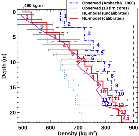
490 kg m−3 according to the average density of the upper-most annual firn layer of 19 density profiles compiled from mountain glaciers in different climatic regimes (Table 1).

it is assumed to mostly take place in the first year after snow deposition and to only have a minor importance for mountain glaciers. The parametercof Eq. 5 is defined as

c=k1(b·ρice/ρw)1/2, (6)

withbthe annual accumulation rate in meters water equiva-lent (w.e.) andρwthe density of water. The termk1is

con-stant for temperate conditions and is given as

k1=f·exp

−21400 RT

, (7)

whereRis the gas constant,T the firn temperature in K, and f a factor that was empirically determined by Herron and Langway (1980). In this study,f is used to tune simulated to observed firn densification (see below).

In order to keep the model simple (not requiring climate data input) and location-independent, firn densification due to refreezingRF (t )(Eq. 5) is roughly approximated by as-suming an end-of-winter firn temperature profile that linearly increases from−5◦C at the firn surface to 0◦C at a depth of 5 m. This profile corresponds to the typical penetration depth of winter air temperatures (e.g. Hooke et al., 1983; and Greuell and Oerlemans, 1989) and defines a negative heat reservoir for refreezing melt water. For each firn layer, re-freezing r is obtained by prescribing complete latent heat exchange. Total refreezingRF (t )after tyr is calculated as RF (t )=RF (t−1)+r. After pore close-off at 830 kg m−3, a linear densification rate with age of 10 kg m−3a−1 is as-sumed until ice density is reached.

Density measurements from 19 firn cores acquired on mountain glaciers or ice caps were compiled for calibrat-ing the firn compaction model (see Table 1 for references). Firn cores reach depths of 10–22 m and are available for the European Alps, Western and Arctic Canada, Central Asia, Patagonia, and Svalbard. Most cores originate from temper-ate firn, but some glaciers are also polythermal. Detailed records that resolve the density of annual layers are provided by a 20 m deep firn pit on Kesselwandferner, Austria (Am-bach and Eisner, 1966). The firn densification regime on this glacier is assumed to be similar as for the Gries- and Sil-vrettagletscher (Fig. 1). All other firn density data were aver-aged in 1 m steps resulting in a representative density–depth relation supported by data from mountain glaciers in differ-ent regions. The standard deviation of observed density is 45–88 kg m−3 over depths of 1–18 m. The data of Kessel-wandferner indicate slightly higher densities compared to the 18-core average profile but pore close-off is reached at the same depth (Fig. 2).

Application of the original HL model including an addi-tional term for refreezing for a location with mean annual accumulation rates equal to those observed by Ambach and Eisner (1966) withf=575 (following Herron and Langway (1980), Eq. 7) results in too-slow firn compaction (Fig. 2). The parameterf=1380 is optimized to match density profiles

1 2

3

4 5 6

7

8

9 10 11

12 1

2

3

4 5

6 7

8 9

10 11

12 13

14

490 kg m-3

500 600 700 800 900

Density (kg m-3)

20 15 10 5 0

Depth (m)

Observed (Ambach&, 1966) Observed (18 firn cores) HL-model (uncalibrated) HL-model (calibrated)

Fig. 2. Validation of calculated firn density (constant accumulation rate) against field measurements. Density of annual layers according to Ambach and Eisner (1966) and a mean density profile from 18 firn cores in different regions worldwide are shown (±1 standard deviation given by grey bars). Numbers indicate the age of the firn layers in years.

obtained from the firn cores (Fig. 2). Densification rates with depth and age observed in different regions worldwide agree well with density calculated with the calibrated HL model indicating that this empirical approach is able to capture firn compaction for a wide range of mountain glaciers and ice caps (Fig. 2).

2.3 Mass balance forcing

In order to force the firn compaction model for the simplified glacier geometries, four experiments of idealized changes in surface mass balance were defined (Fig. 3). Each experiment consists of two scenarios, with a positive and a negative shift in ELA, respectively. Before applying a change in mass bal-ance, the model is run for a 50 yr spin-up phase with the ELA that yields a balanced mass budget. This allows convergence of the firn density profile to an equilibrium.

Surface mass balance distribution is prescribed by two lin-ear elevation gradients db/dz. For the ablation area db/dz=

0.008 a−1is assumed, and db/dz=0.004 a−1 is chosen for the accumulation area. These values correspond to typically observed mass balance gradients on midlatitude mountain glaciers (e.g. WGMS, 2008). Four specific experiments are performed, and their characteristics are visualized in Fig. 3.

-1 0 1

0

Mass balance (m w.e.)

Experiment I

a

50 years 100 years

0

Elevation

Mass balance

-1 0 1

0

Mass balance (m w.e.)

Experiment II

b

50 years 100 years

0

Elevation

Mass balance

-1 0 1

0

Mass balance (m w.e.)

Experiment III

c

50 years 100 years

0

Elevation

Mass balance

-1 0 1

0

Mass balance (m w.e.)

Experiment IV

d

50 years 100 years

0

Elevation

Mass balance

Fig. 3. Four experiments of surface mass balance forcing. Time series of glacier-wide mass balance (left), and mass balance dis-tribution with elevation (right) are shown for each experiment. An experiment consists of two scenarios with a positive (red) and a neg-ative (blue) shift in equilibrium line altitude.

– Experiment II: a linear increase/decrease in ELA by

5 m a−1is prescribed.

– Experiment III: the step changes in mass balance are

limited but the spatial distribution is changed. Whereas the first scenario assumes a 50 % increase in mass bal-ance gradients both in the ablation and the accumula-tion area, the second scenario is characterized by re-duced gradients. Both scenarios also include a small positive/negative shift in ELA.

– Experiment IV: a+100/−100 m shift in ELA (similar to Experiment I) is applied but a natural year-to-year variability in mass balance is superimposed.

Surface mass balance forcing for the case studies on Gries-and Silvrettagletscher is provided by gridded maps of the annual mass balance distribution based on the extrapola-tion of the in situ measurements for the period 1961–2007, and 1959–2007, respectively (Huss et al., 2009). The glacier geometry is updated annually taking into account surface lowering and glacier retreat based on direct observations.

Both glaciers showed a balanced mass budget between the beginning of the measurements and the 1980s, and strong mass loss afterwards (Huss et al., 2009). Over the two-decadal period 1987–2007, the mean annual balance was B20= −1.15 m w.e. for Gries, and B20= −0.66 m w.e. for

Silvretta with the ELA above the highest point of the accu-mulation area in several years causing a substantial degrada-tion of the firn coverage (Fig. 1).

For both the synthetic glaciers and the case studies, mass change 1M is calculated by integrating surface mass bal-ance over the glacierized area. Volume change 1V is ob-tained from the integration of firn layer thickness changes provided by the densification model over the entire firn col-umn. For the ablation area, ice density is assumed to be con-stant atρice=900 kg m−3 for calculating volume changes.

Thus, Eq. (1) can be solved and the conversion factorf1V

between volume change and mass change can be calculated for arbitrary periods of one year to several decades.

3 Results

3.1 f1V for idealized glaciers

For each of the four experiments (Fig. 3), the combined model for surface mass balance forcing and firn compaction is run, providing annual series of the change in glacier mass and volume. Figure 4 shows the conversion factorf1V for

observation periods of geodetic volume change that start with the step change in climate forcing and increase in length from 1 to 50 yr.

After a shift in ELA,f1V converges towards 900 kg m−3

after some decades. When the firn density profile is allowed sufficient time to adapt, the cumulative volume loss in the ablation area (withρice) tends to dominate the changes in the

firn area. For periods shorter than about two decades,f1V

can however be significantly lower than 900 kg m−3 (Ex-periment I), both in the case of positive and negative vol-ume change (Fig. 4a, Table 2). Firn layers with a density smaller than ρice are added/removed which tends to make

the glacier volume change larger than implied by the first or-der approximation off1V =ρice, irrespective of the sign of

mass balance change. This is also evident from Eq. (4) pro-viding details on the components off1V. For example, a

re-duction in firn coverage associated with a negative volume change (1V <0) leads to an increase in bulk glacier den-sity (1ρ >0), and thus a value off1V smaller than average

glacier densityρ.

For a linearly increasing/decreasing mass balance (Ex-periment II),f1V shows a similar evolution as for

0 10 20 30 40 50 750

800 850 900 950

Conversion factor f

dV

(kg m

-3 )

Experiment I

a

Experiment + (ELA increase)

Experiment - (ELA decrease)

0 10 20 30 40 50

750 800 850 900 950

Experiment II

b

0 10 20 30 40 50

Observation period length (years) 900

1000 1100 1200

Conversion factor f

dV

(kg m

-3 )

Experiment III

c

Higher dB/dz

Lower dB/dz

0 10 20 30 40 50

Observation period length (years) 750

800 850 900 950

Experiment IV

d

Fig. 4. Calculated conversion factorf1V for observation period lengths increasing from 1 to 50 yr after a change in mass balance (Fig. 3).

Thin grey lines refer to model runs using different glacier size (elevation ranges 300–2000 m), solid lines show the mean of all experiment simulations for a positive/negative shift in the ELA. In (d) the variability of 200 model runs is expressed as their average±2 standard deviations (shaded areas). Selected series off1V for individual model runs are shown.

after the spin-up phase (1ELA=5 m),f1V significantly

di-verges from 900 kg m−3(Fig. 4b). This indicates that assum-ing validity of Sorge’s law for estimatassum-ing the factor to con-vert volume change to mass change is not even feasible for a small shift in mass balance forcing although the absolute error in calculated mass change would be limited for any con-version factor.

Experiment III highlights a particular case that yields sur-prising results. If mass balance gradients both in the ab-lation and the accumuab-lation area show a significant in-crease/decrease together with a relatively small change in glacier-wide mass balance,f1V can assume values

signifi-cantly larger than the density of water (Fig. 4c, Table 2). Ab-solute glacier volume changes are thus smaller than the asso-ciated mass changes in m3w.e. For the case of increasing gra-dients (Experiment III+), volume loss withρiceis enhanced

in the ablation zone, whereas the firn volume with a low av-erage density grows in the accumulation area, partly com-pensating for the ice melt below the ELA. Strongly chang-ing mass balance gradients are a rather particular response of glaciers to climate change, but may occur with rapidly

rising air temperatures simultaneous to a precipitation in-crease as it has recently been observed in Arctic regions (e.g. Abdalati et al., 2005).

“Densities” of glacier volume change higher than 900 kg m−3seem to be unphysical at first glance. However, the conversion factor f1V does not necessarily correspond

to the physical properties of a density (see also Eq. 4). For example, a glacier volume change (1V 6=0) can occur with-out any change in mass (1M=0) purely due to compaction of the firn layers. Conversely, mass balance can be negative (1M6=0) with no change in total volume (1V =0) if melt increases in the ablation area, compensated in terms of vol-ume by higher accumulation in the firn zone. According to Eq. (1) it is evident that for such special cases,f1V can

the-oretically be located in the range [−∞,∞], i.e. it can even be negative if the signs of mass change and volume change are opposite.

Experiment IV is based on a variable mass balance forc-ing and thus most closely represents real conditions (Fig. 3). Averagef1V over 200 model runs of different random

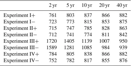
Table 2. Calculated conversion factorf1V (in kg m−3) for all

ex-periments (Fig. 3) and different lengths of the observation period (in years) after a change in mass balance. Scenarios with a positive (+) and a negative (−) shift in ELA are shown.

2 yr 5 yr 10 yr 20 yr 40 yr

Experiment I+ 761 803 837 866 882

Experiment I− 723 773 815 853 875

Experiment II+ 715 747 785 828 863 Experiment II− 712 741 774 811 842 Experiment III+ 1720 1405 1139 1007 950 Experiment III− 1589 1281 1085 984 939 Experiment IV+ 784 805 838 866 882

Experiment IV− 752 782 817 855 876

conversion factor increases gradually from about 770 kg m−3 towards ice density with increasing observation period length (Table 2). For individual series of variable mass balance forc-ing, a strongly fluctuating signal is found however, in partic-ular for observation period lengths of≤3 yr (Fig. 4d). The interplay of years with positive and negative mass balance leads to a complex pattern of the firn densification dynamics in which anomalous accumulation can impact on compaction rates for several years after deposition. If annual or multi-annual mass change is close to zero, already small changes in the firn density profile can induce diverging responses of glacier volume and mass, and hence a conversion factorf1V

that is highly variable and difficult to estimate.

The dependence off1V on glacier size was analysed by

repeated individual model runs for glacier geometries for el-evation ranges of 300–2000 m (100 m steps). In general, the conversion factor shows similar trends for small and large glaciers although some spread is evident (Fig. 4). Whereas for scenarios with negative glacier mass balance, the eleva-tion range has little influence onf1V (around±10 kg m−3),

the effect is more pronounced for an increase in ice volume. Glaciers with a limited elevation range, in particular, can show values off1V smaller by up to 80 kg m−3 compared

to large glaciers. This is due to the higher percentage of the area of small glaciers that is affected by a given shift in the ELA. Elevation range is more influential for Experiment III; f1V of small glaciers is belowρice(Fig. 4c) because they do

not reach a critical size of the accumulation area.

Although all experiments for the synthetic glaciers indi-cate a significant dependence off1V on the period

consid-ered (Fig. 4), a general statement about a representative value of the volume–mass conversion factor and the related uncer-tainties is possible with some restrictions. By averaging cal-culatedf1V for time intervals of 5–50 yr (typical for

geode-tic mass balance determination) and the Experiments I, II and IV, a mean value off1V =850 kg m−3is found. Based on a

combined assessment of the effect of glacier size and differ-ences inf1V for short and multi-decadal periods, an

uncer-tainty range of±60kg m−3is assigned. In the case of (i) peri-ods shorter than 5 yr, (ii) significant changes in the mass bal-ance gradients (e.g. Experiment III), (iii) small overall vol-ume changes, or (iv) an insignificant firn area, this average conversion factor might however not be applicable andf1V

can lie beyond the specified uncertainty ranges. If the above caveats are accounted for, 850±60 kg m−3is recommended for converting volume change to mass change for studies that do not perform an in-depth analysis of changes in firn volume and density.

3.2 Application to long-term series

f1V is computed based on a spatially distributed run of the

firn compaction model using each year’s observed mass bal-ance distribution for Gries- and Silvrettagletscher as input af-ter a spin-up phase. Calculated firn thickness locally reaches 20 m and shows a pattern related to the spatial variability of surface accumulation rates (Fig. 1). In response to a se-ries of very negative mass balance years after the late 1980s (Glaciological Reports, 1960–2011), the thickness of the firn coverage has strongly decreased on Silvretta, and it has al-most disappeared on Gries.

Comparison of observed mass balance and calculated vol-ume change for individual years of the fluctuating signal shows that the annual conversion factor is subject to strong variability (Fig. 5a, b). This corresponds to the results of Ex-periment IV (Fig. 4d), and indicates that determining glacier mass balance from short-term (i.e. one to a few years) geode-tic surveys might be prone to errors due to an uncertain con-version of volume change to mass change.

Evaluation of the complete series of annual conversion factors for both glaciers (n=92) shows thatf1V ranges

be-tween minimum/maximum values of−500 and 6500 kg m−3 for annual mass balances Ba of −0.2 to +0.2 m w.e. a−1

indicating a large relative uncertainty in the estimation of f1V for small mass changes. The spread in f1V rapidly

reduces with increasing magnitude of mass change being 790±75 kg m−3for|Ba|>1 m w.e. a−1. By multiplying the

deviation of annually evaluatedf1V from a reference value

of 850 kg m−3with that year’s mass balance, a maximum ac-curacy for the geodetic annual determination of mass change can be estimated. It is found that for Gries- and Silvretta-gletscherBais subject to an uncertainty greater than at least ±0.05 m w.e. a−1due to the variability inf1V.

f1V was also determined by driving the firn compaction

model with observed mass balance for periods of between 4 and 14 yr corresponding to the dates of available DEMs. This allows validating assumptions on the volume–mass con-version factor made in previous evaluations of the time se-ries (Huss et al., 2009), and illustrates characteristic val-ues of f1V in applied mass balance monitoring of

Mass change (10 9 kg a -1)/ Volume change (10 6 m 3 a -1)

Conversion factor f

dV (kg m -3 )

a

Gries

833 ₈₂₅ 875 880

-15 -10 -5 0 5 Volume change Mass change

b

Silvretta

412 138 585 887 750 1015 891 -10 -8 -6 -4 -2 0 2

1990 1995 2000 2005

Mean specific mass balance (m w.e. a

-1)

Conversion factor f

dV (kg m -3 )

c

d

1960 1970 1980 1990 2000

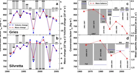
Fig. 5. Annual series of observed mass change and calculated volume change between 1990 and 2005 for (a) Griesgletscher and (b) Silvrettagletscher. The conversion factorf1V for each year’s volume change is shown by bars. Note that for bars beyond the plotted range,

values are stated. (c), (d)f1V for Gries and Silvretta over period lengths of 4–14 yr corresponding to the dates of DEMs, and observed mean

specific mass balances as period averages. Blue lines showf1V ,zonalestimated assuming zonally separated “densities” of volume change

(see e.g. Moholdt et al., 2010).

range 777–892 kg m−3 (Fig. 5c, d). With ongoing climate change, the firn coverage of small to medium-sized moun-tain glaciers might completely disappear, resulting in af1V

converging to ice density. From the 1960s to the early 1980s, with mean mass balances close to zero, much more variable values are found for decadal periods. Reduced “densities” of volume change prevailing during these decades are explained by increased accumulation rates leading to the build-up of thick low-density firn layers, and thus relatively large volume changes compared to the almost balanced mass budget.

f1V is 878 kg m−3for Gries, and 866 kg m−3for Silvretta

for the entire 5-decadal observation period. Considering the components off1V (Eq. 4), these numbers seem to be

rea-sonable given a bulk glacier density ρ of slightly below 900 kg m−3(volume-weighted average of mean firn and ice densities), and the changes in glacier density1ρand volume 1V over time.

The suitability of using separate conversion factors for volume changes in the accumulation and the ablation area (e.g. Moholdt et al., 2010; Kaeaeb et al., 2012; and Bolch et al., 2013) was assessed by evaluating zonal surface eleva-tion changes between two DEMs. Geodetic mass change was calculated using a “density” of volume change of 600 kg m−3 in the firn area, and 900 kg m−3below. Resulting changes in overall mass and volume were compared providingf1V ,zonal

for all decadal periods (Fig. 5c, d). This relatively simple

ap-proach that avoids assuming a constant volume–mass conver-sion factor over time is able to reproduce some of the decadal variability inf1V found with the firn compaction model. It

does, however, not take into account that changes in firn vol-ume and density might not be revealed as variations in sur-face elevation due to ice flow dynamics. Hence, this method only captures part of the effect and might underestimate the uncertainties.

4 Discussion

Although Figs. 4 and 5 suggest that values off1V may be

small absolute errors in calculated mass change as they oc-cur in connection to an almost balanced mass budget (Fig. 5). Significant changes in mass balance gradients (iii) with a lim-ited magnitude of glacier mass loss/gain (Fig. 3c) are related to a major shift in climatic conditions. This particular case needs to be carefully addressed if there are hints that these constraints are met. By accounting for the three above re-strictions in the application of the geodetic method, problems arising from an uncertain conversion factor can be tackled and be reduced to an acceptable level.

All evaluations presented in this paper refer to land-terminating glaciers. Ice volume loss by calving is not in-cluded in the model and would require the explicit descrip-tion of ice flow dynamics. General concepts, such as the dependence off1V on the time period considered, and the

high variability of the conversion factor for particular cases, are however assumed to be valid for marine-terminating glaciers as well.

Several sensitivity tests were performed to investigate the robustness of calculated f1V on changes in the synthetic

glacier geometries and simplifications in the modelling of firn densification. The model was run with idealized mass balance forcing for all experiments (Fig. 3). Differences in the computed conversion factor were compared to the “refer-ence” results (shown in Fig. 4 and Table 2) and outcomes are discussed hereafter.

In a first experiment, additional synthetic glaciers were defined for analysing the dependence off1V on glacier

ge-ometry: (1) the glacier with a constant width has a slope of 8◦ below half of its elevation range, and is steep (35◦) in its upper reaches; (2) it is inclined by 35◦ _{in the ablation}

area, and 8◦ _{in the accumulation area; and (3) the width of}

the accumulation area is increased by a factor 5 relative to the ablation area (with a constant slope of 15◦). The area– elevation distribution of the glacier has a small influence on f1V. Slightly higher average values were found for a glacier

exhibiting a steep firn zone (+1 kg m−3, excluding Experi-ment III), and lowerf1V is present for the glacier geometry

with a steep ablation area (−18 kg m−3). Increasing the width of the accumulation area yields a difference in averagef1V

of−19 kg m−3.

Assessing the performance and the suitability of the HL model for mountain glaciers is difficult due to the paucity of direct field evidence (the parameters of Eq. (5) are poorly constrained). To test the impact of the approach to model firn compaction on calculatedf1V, a simple linear firn density

change with age fitted to the mean observed density pro-file was considered. Assuming a constant densification rate of 35 kg m−3a−1 yields results for f1V that are lower by

15 kg m−3on average (excluding Experiment III) compared to the reference. Varying the initial firn density ρfirn,0

be-tween the minimum and the maximum of the observed values (Table 1) leads to changes inf1V of−31 and+26 kg m−3,

respectively.

The sensitivity off1V on the climate regime, i.e. the

sur-face mass balance distribution, and potential changes in char-acteristic compaction rates with higher temperatures, was analysed (i) by reducing balance gradients by a factor 2 for all experiments, corresponding to more continental condi-tions, and (ii) by increasing the amount of refreezingRF (t ) (Eq. 5) by 100%. The approach to modelf1V is relatively

insensitive even to these major changes in firn compaction. For reduced mass balance gradients, the average conversion factor is 10 kg m−3 below the reference results (excluding Experiment III). Doubling the refreezing rateRF (t )causes an increase in averagef1V by+20 kg m−3. More

refreez-ing is expected in a warmrefreez-ing climate for cold or polythermal glaciers (e.g. Zdanowicz et al., 2012). For temperate moun-tain glaciers, higher temperatures will however rather reduce RF (t ).

The sensitivity tests indicate that calculatedf1V is robust

regarding glacier geometry, the approach to model firn densi-fication, and the climatic regime (continental/maritime). The conversion factor for most sensitivity tests is slightly below the reference results, but shows the same temporal trends and remains in the range of 700–900 kg m−3. The calcu-lated averagef1V for Experiment III is higher, in contrast,

for some sensitivity runs as they generally yield lower com-paction rates thus exaggerating the firn volume response to a given mass balance forcing. However, the simplified set-ting of the experiments cannot account for all influential pro-cesses present in nature. For example, densification due to refreezing is only modelled crudely although major changes in the firn density profile of polythermal glaciers due to this process have been reported related to ongoing climate change (Zdanowicz et al., 2012).

Besides the process of firn compaction that was explicitly modelled in this study, other effects can also influence the “density” of glacier volume change. Fischer (2011) describes the impact of opening and closure of crevasses on geode-tic volume change in detail. If many crevasses are present, the bulk density of the entire ice body decreases. Changes in crevasse frequency over time might lead to a bias in the con-version of volume to mass. The importance of this effect also depends on the timing (snow coverage) and the spatial res-olution of the geodetic survey. Although this process might affectf1V, its magnitude is difficult to quantify and needs to

be addressed for each case individually.

5 Conclusions

for two long-term glacier monitoring programs. The conver-sion factorf1V is, in most cases, below the ice density which

is used in numerous studies for calculating mass balance from geodetic volume change. The effect is relatively small, yielding a typical overestimate of mass change of roughly 2–15 %, but it is systematic, and thus needs to be accounted for. For observation periods of some years to several decades featuring significant changes in glacier volume, the density of volume change often lies in the range of 780–880 kg m−3, both for positive and negative mass balances. For the particu-lar case of strong changes in mass balance gradients together with limited mass gain/loss,f1V can however also be

sys-tematically higher than the ice density as opposite signs of elevation changes in the accumulation and the ablation area can compensate for each other in terms of volume. If short time intervals (1–3 yr) in a fluctuating mass balance signal are considered, and/or the volume changes over the observa-tion period are small,f1V can show an erratic behavior and

may assume values of 0–2000 kg m−3and beyond.

The findings of this study are in line with the simple as-sessment of f1V by Sapiano et al. (1998) but highlights

the strong variability, the underlying processes and the prob-lems inherent to assuming a constant factor to convert geode-tic glacier volume change to mass change. f1V =850±

60 kg m−3is recommended in the case of periods longer than 5 yr, with stable mass balance gradients, the presence of a firn area, and volume changes significantly different from zero. The conversion factor can however strongly diverge from this mean value for particular conditions, and the density assump-tion might represent a significant component of uncertainty in geodetically determined mass balances that is larger than previously assumed.

Acknowledgements. This study was triggered by discussions at a WGMS organized workshop on the “measurement and uncer-tainty assessment of glacier mass balance” held at Tarfala, Sweden, in July 2012. M. Funk and M. Hoelzle provided helpful comments on an earlier version of the manuscript. Reviews by an anonymous reviewer and G. Moholdt contributed to the quality of the paper.

Edited by: M. Van den Broeke

References

Abdalati, W., Krabill, W., Frederick, E., Manizade, S., Mar-tin, C., Sonntag, J., Swift, R., Thomas, R., Yungel, J., and Koerner, R.: Elevation changes of ice caps in the Cana-dian Arctic Archipelago, J. Geophys. Res., 109, F04007, doi:10.1029/2003JF000045, 2005.

Abermann, J., Fischer, A., Lambrecht, A., and Geist, T.: On the potential of very high-resolution repeat DEMs in glacial and periglacial environments, The Cryosphere, 4, 53–65, doi:10.5194/tc-4-53-2010, 2010.

Ambach, W. and Eisner, H.: Analysis of a 20 m firn pit on the Kesselwandferner ( ¨Otztal Alps), J. Glaciol., 6, 223–231, 1966.

Arthern, R. and Wingham, D.: The natural fluctuations of firn den-sification and their effect on the geodetic determination of ice sheet mass balance, Climatic Change, 40, 605–624, 1998. Bader, H.: Sorge’s law of densification of snow on high polar

glaciers, J. Glaciol., 2, 319–323, 1954.

Bamber, J. L. and Rivera, A.: A review of remote sensing methods for glacier mass balance determination, Global Planet. Change, 59, 138–148, 2007.

Bauder, A., Funk, M., and Huss, M.: Ice volume changes of selected glaciers in the Swiss Alps since the end of the 19th century, Ann. Glaciol., 46, 145–149, 2007.

Bolch, T., Sandberg Sørensen, L., Simonsen, S. B., M¨olg, N., Machguth, H., Rastner, P., and Paul, F.: Mass loss of Green-land’s glaciers and ice caps 2003–2008 revealed from ICE-Sat laser altimetry data, Geophys. Res. Lett., 40, 875–881, doi:10.1002/grl.50270, 2013.

Breili, K. and Rolstad, C.: Ground-based gravimetry for measuring small spatial-scale mass changes on glaciers, Ann. Glaciol., 50, 141–147, 2009.

Cogley, J. G.: Geodetic and direct mass balance measurements: comparison and joint analysis, Ann. Glaciol., 50, 96–100, 2009. Cox, L. H. and March, L. S.: Comparison of geodetic and glacio-logical mass-balance techniques, Gulkana Glacier, Alaska, USA, J. Glaciol., 50, 63–70, 2004.

Cuffey, K. M. and Paterson, W. S. B.: The Physics of Glaciers, 4. edn., Butterworth-Heinemann, Oxford, 704 pp., 2010. Fischer, A.: Glaciers and climate change: Interpretation of 50 years

of direct mass balance of Hintereisferner, Global Planet. Change, 71, 13–26, 2010.

Fischer, A.: Comparison of direct and geodetic mass balances on a multi-annual time scale, The Cryosphere, 5, 107–124, doi:10.5194/tc-5-107-2011, 2011.

Gardelle, J., Berthier, E., and Arnaud, Y.: Slight mass gain of Karakoram glaciers in the early twenty-first century, Nat. Geosci., 5, 322–325, doi:10.1038/ngeo1450, 2012.

Glaciological Reports: The Swiss Glaciers, 1958/59–2006/07, No. 80–128, Yearbooks of the Cryospheric Commission of the Swiss Academy of Sciences (SCNAT), Laboratory of Hy-draulics, Hydrology and Glaciology (VAW) of ETH Z¨urich, 1960–2011.

Greuell, J. and Oerlemans, J.: The evolution of the englacial temper-ature distribution in the superimposed ice zone of a polar ice cap during a summer season, in: Proceedings of the Symposium on glacier fluctuations and climatic change, edited by: Oerlemans, J., Kluwer Academic Publishers, Dordrecht, 289–304, 1989. He, Y., Yao, T., Theakstone, W., Cheng, G., Yang, M., and Chen, T.:

Recent climatic significance of chemical signals in a shallow firn core from an alpine glacier in the South-Asia monsoon region, J. Asian Earth Sci., 20, 289–296, 2002.

Helsen, M. M., van den Broeke, M. R., van de Wal, R. S. W., van de Berg, W. J., van Meijgaard, E., Davis, C. H., Li, Y., and Goodwin, I.: Elevation changes in Antarctica mainly de-termined by accumulation variability, Science, 320, 1626–1629, doi:10.1126/science.1153894, 2008.

Herron, M. M. and Langway, C. C.: Firn densification: an empirical model, J. Glaciol., 25, 373–385, 1980.

1–25, 1983.

Huss, M., Bauder, A., and Funk, M.: Homogenization of long-term mass balance time series, Ann. Glaciol., 50, 198–206, 2009. Jacob, T., Wahr, J., Pfeffer, W. T., and Swenson, S.: Recent

con-tributions of glaciers and ice caps to sea level rise, Nature, 482, 514–518, doi:10.1038/nature10847, 2012.

Kaeaeb, A., Berthier, E., Nuth, C., Gardelle, J., and Ar-naud, Y.: Contrasting patterns of early twenty-first-century glacier mass change in the Himalayas, Nature, 488, 495–498, doi:10.1038/nature11324, 2012.

Kaser, G., Fountain, A., and Jansson, P.: A manual for monitoring the mass balance of mountain glaciers, UNESCO, 2003. Kawashima, K. and Yamada, T.: Experimental studies on the

trans-formation from firn to ice in the wet-snow zone of temperate glaciers, Ann. Glaciol., 24, 181–185, 1996.

Kreutz, K. J., Aizen, V. B., Dewayne Cecil, L., and Wake, C. P.: Oxygen isotopic and soluble ionic composition of a shallow firn core, Inilchek glacier, central Tien Shan, J. Glaciol., 47, 548–554, 2001.

Li, J. and Zwally, H. J.: Modeling the density variation in the shal-low firn layer, Ann. Glaciol., 38, 309–313, 2004.

Ligtenberg, S. R. M., Helsen, M. M., and van den Broeke, M. R.: An improved semi-empirical model for the densification of Antarc-tic firn, The Cryosphere, 5, 809–819, doi:10.5194/tc-5-809-2011, 2011.

Matsuoka, K. and Naruse, R.: Mass balance features derived from a firn core at Hielo Patag´onico Norte, South America, Arct., Antarct. Alp. Res., 31, 333–340, 1999.

Moholdt, G., Nuth, C., Hagen, J. O., and Kohler, J.: Recent elevation changes of Svalbard glaciers derived from ICESat laser altimetry, Remote Sens. Environ., 114, 2756–2767, 2010.

Nuth, C., Moholdt, G., Kohler, J., Hagen, J. O., and K¨a¨ab, A.: Svalbard glacier elevation changes and contribution to sea level rise, J. Geophys. Res., 115, F01008, doi:10.1029/2008JF001223, 2010.

Oerter, H., Reinwarth, O., and Rufli, H.: Core drilling through a temperate Alpine glacier (Vernagtferner, Oetztal Alps) in 1979, Zeitschrift f¨ur Gletscherkunde und Glazialgeologie, 18, 1–11, 1982.

P¨alli, A., Kohler, J. C., Isaksson, E., Moore, J. C., Pinglot, J. F., Pohjola, V. A., and Samuelsson, H.: Spatial and temporal vari-ability of snow accumulation using ground-penetrating radar and ice cores on a Svalbard glacier, J. Glaciol., 48, 417–424, 2002. Paul, F. and Haeberli, W.: Spatial variability of glacier

ele-vation changes in the Swiss Alps obtained from two dig-ital elevation models, Geophys. Res. Lett., 35, L21502, doi:10.1029/2008GL034718, 2008.

Reeh, N.: A nonsteady-state firn-densification model for the per-colation zone of a glacier, J. Geophys. Res., 113, F03023, doi:10.1029/2007JF000746, 2008.

Reijmer, C. H. and Hock, R.: Internal accumulation on Stor-glaci¨aren, Sweden, in a multi-layer snow model coupled to a dis-tributed energy- and mass-balance model, J. Glaciol., 54, 61–72, 2008.

Rignot, E., Rivera, A., and Casassa, G.: Contribution of the Patag-onia Icefields of South America to sea level rise, Science, 302, 434–437, doi:10.1126/science.1087393, 2003.

Sapiano, J., Harrison, W. D., and Echelmeyer, K. A.: Elevation, vol-ume and terminus changes of nine glaciers in North America, J. Glaciol., 44, 119–135, 1998.

Schiefer, E., Menounos, B., and Wheate, R.: Recent volume loss of British Columbian glaciers, Canada, Geophys. Res. Lett., 34, L16503, doi:10.1029/2007GL030780, 2007.

Schneider, T. and Jansson, P.: Internal accumulation in firn and its significance for the mass balance of Storglaci¨aren, Sweden, J. Glaciol., 50, 25–34, 2004.

Sharp, R. P.: Features of the firn on Upper Seward Glacier St. Elias Mountains, Canada, J. Geol., 59, 599–621, 1951.

Shiraiwa, T., Kohshima, S., Uemura, R., Yoshida, N., Matoba, S., Uetake, J., and Angelica Godoi, M.: High net accumulation rates at Campo de Hielo Patag´onico Sur, South America, revealed by analysis of a 45.97 m long ice core, Ann. Glaciol., 35, 84–90, 2002.

Sørensen, L. S., Simonsen, S. B., Nielsen, K., Lucas-Picher, P., Spada, G., Adalgeirsdottir, G., Forsberg, R., and Hvidberg, C. S.: Mass balance of the Greenland ice sheet (2003-2008) from ICE-Sat data - the impact of interpolation, sampling and firn density, The Cryosphere, 5, 173–186, doi:10.5194/tc-5-173-2011, 2011. Suslov, V. and Krenke, A.: Lednik Abramov, Hydromet Publishing,

1980.

Thibert, E., Blanc, R., Vincent, C., and Eckert, N.: Glaciological and volumetric mass balance measurements error analysis over 51 years for the Sarennes glacier, French Alps, J. Glaciol., 54, 522–532, 2008.

Vimeux, F., Ginot, P., Schwikowski, M., Vuille, M., Hoffmann, G., Thompson, L. G., and Schotterer, U.: Climate variability dur-ing the last 1000 years inferred from Andean ice cores: a review of methodology and recent results, Palaeogeogr. Palaeocl., 281, 229–241, 2009.

WGMS: Fluctuations of Glaciers, 2000–2005, Vol. IX, ICSU(FAGS)/IUGG(IACS)/UNEP/UNESCO/WMO, World Glacier Monitoring Service, Zurich, Switzerland, 2008. Zdanowicz, C., Smetny-Sowa, A., Fisher, D., Schaffer, N., Copland,

L., Eley, J., and Dupont, F.: Summer melt rates on Penny Ice Cap, Baffin Island: Past and recent trends and implications for regional climate, Journal of Geophysical Research: Earth Surface, 117, F02006, doi:10.1029/2011JF002248, 2012.

Zemp, M., Jansson, P., Holmlund, P., G¨artner-Roer, I., Koblet, T., Thee, P., and Haeberli, W.: Reanalysis of multi-temporal aerial images of Storglaci¨aren, Sweden (1959–99) – Part 2: Com-parison of glaciological and volumetric mass balances, The Cryosphere, 4, 345–357, doi:10.5194/tc-4-345-2010, 2010. Zemp, M., Thibert, E., Huss, M., Stumm, D., Rolstad Denby, C.,